Measurement of energy eigenstates by a slow detector

Abstract

We propose a method for a weak continuous measurement of the energy eigenstates of a fast quantum system by means of a “slow” detector. Such a detector is only sensitive to slowly-changing variables, e. g. energy, while its back-action can be limited solely to decoherence of the eigenstate superpositions. We apply this scheme to the problem of detection of quantum jumps between energy eigenstates in a harmonic oscillator.

Observation of quantum mechanical behavior of macro-scale systems is one of the most fascinating current problems in physics. Several successes have been claimed so far. They include observation of avoided crossing between counter-propagating current states in Josephson loops lukens , coherent evolution of macroscopic quantum states in charge nakamura and phase martinis qubits, and interference experiments on very large molecules zeilinger .

Recently, experiments on fabricated nano-mechanical systems became feasible roukes , with the position measurement resolution approaching the zero-point motion uncertainty schwab . However, the commonly used linear position measurement has fundamental limitations due to the measurement apparatus back-action, which ultimately drives the oscillator away from the quantum regime caves ; mozyrsky ; clerk . Thus a question naturally arises whether it is feasible to observe quantum behavior of nanomechanical systems by means of a non-linear measurement procedure. Specifically, since the oscillator energy is quadratic in displacement $x$, coupling the measurement apparatus to $x^{2}$ can naturally lead to the measurement and projection into the energy eigenstates. The main difficulty with this approach is that such coupling requires very precise tuning santamore in order to eliminate the linear-$x$ coupling which would otherwise dominate at small displacements.

There is an intimate connection between the measurement process and interaction with a general extrinsic environment since both represent coupling of a system to a macroscopically large number of degrees of freedom. The practical difference is that the classical output of the measurement apparatus (or “meter”) is available to the observer, and thus one can ask questions, e.g. about the signal to noise ratio, that is how much of the output can be attributed to the system that one is measuring, and how much to the noise of the apparatus bragisnky . Depending on the relative strengths of the system’s coupling to the environment and to the measurement apparatus, its own behavior can be either predominantly affected by the environment (einselection) zurek or by the meter. The latter case is typically equivalent to coupling to a non-equilibrium environment, which nevertheless can result in a crossover to effectively thermal behavior of the system with the “temperature” determined by the degree of non-equilibrium in the meter (e.g. bias voltage in a quantum point contact mozyrsky ).

When environment is weakly coupled to the system and is slow compared to the intrinsic system dynamics (determined by its self-hamiltonian $H_{0}$), an interesting possibility arises: While the environment can lead to the decoherence of superpositions of the energy eigenstates, it can not effectively cause transitions between them. This is a consequence of the quantum adiabatic theorem. Decoherence is commonly associated with a gradual projection into one of the states of the superposition. Thus one concludes that the system should remain in the energy eigenstates paz most of the time, with the rare transitions (quantum jumps, QJ) between them governed by the residual relaxation processes. A necessary condition for this scenario is a presence of non-zero diagonal (in the energy eigen-basis) coupling between environment and the system, which leads to environment-induced fluctuations in the system level spacing.

In this Letter we apply the ideas of slow environment to the measurement process and determine the circumstances under which QJ should become observable. We perform analysis for a harmonic oscillator playing the role of the quantum system being measured, with the Hamiltonian

$$H_{o}=\frac{p^{2}}{2m}+\frac{m\omega_{0}^{2}x^{2}}{2},$$

where $x$ is the oscillator position, $p$ is the momentum, $m$ is its mass and $\omega_{0}$ is its frequency. Analysis for a more general systems is similar. For harmonic oscillator, the requirement on non-zero diagonal coupling is equivalent to inclusion of non-linear terms in the meter-oscillator coupling. For concreteness we consider terms up to quadratic order in displacement,

$$H_{\rm int}=(\lambda_{1}x+\lambda_{2}x^{2})\mathcal{F}\equiv\Omega(x)\mathcal{F}.$$ (1)

Note that for a slow operator $\mathcal{F}$ the linear coupling term ($\lambda_{1}$) does not generate non-linear in $x$ terms within perturbation theory.

We will first derive the measurability criteria for QJ for a general measurement apparatus that interacts with the oscillator via operator $\mathcal{F}$ and generates output $I$. We will then give a specific example of such a measurement when a single electron transistor (SET) is capacitively coupled to the oscillator. This experimental procedure is closely related to the displacement measurement techniques currently in use schwab .

The complete Hamiltonian for the combined system of the oscillator and the measurement apparatus (meter) consists of three parts,

$$H=H_{o}+H_{M}+H_{\rm int}$$ (2)

with $H_{o}$ and $H_{\rm int}$ specified above and $H_{M}$ being the Hamiltonian of the meter. The evolution of the full density matrix $\rho$ is given by $\dot{\rho}=i[\rho,H]$. Assuming that the interaction between the measurement apparatus and the system is relatively weak, that is it dominates neither the oscillator’s dynamics nor the meter’s (“weak measurement”), we can determine the evolution by means of the perturbation theory. In the interaction representation, where $\hat{\rho}=e^{-i(H_{0}+H_{M})t}\rho e^{i(H_{0}+H_{M})t}$ and $\hat{H}_{\rm int}=e^{i(H_{0}+H_{M})t}H_{\rm int}e^{-i(H_{0}+H_{M})t}$, the second-order perturbation theory yields,

$$\dot{\hat{\rho}} = i[\hat{\rho},\hat{H}_{\rm int}]=i{[\rho(0)+i\int_{0}^{t}dt^{\prime}[\hat{\rho},\hat{H}_{\rm int}]_{t^{\prime}},\hat{H}_{\rm int}]}$$ (3)

$$\approx i[\rho(0),H_{\rm int}]-\int_{0}^{t}{dt^{\prime}[[\hat{\rho},\hat{H}_{\rm int}(t^{\prime})],\hat{H}_{\rm int}]}$$ (4)

Here the operators with unspecified time variable are taken at time $t$. The final step is equivalent to the Markovian approximation, which is valid if the time correlations in $\hat{H}_{\rm int}$ decay faster than the decay times of diagonal and off-diagonal elements of the density matrix (in the jargon of nuclear magnetic resonance, the times $T_{1}$ and $T_{2}$, respectively). Making now the common assumption that the initial density matrix is factorizable, $\rho(0)=\rho_{o}(0)\bigotimes\rho_{M}(0)$, and tracing over the meter density matrix $\rho_{M}$ we can obtain the evolution of the reduced density matrix of the oscillator $\rho_{o}$.

$$\dot{\hat{\rho}}_{o} = i[\hat{\rho}_{o},\hat{\Omega}]\langle\hat{\mathcal{F}}\rangle$$

$$- \int_{0}^{t}dt^{\prime}[[\hat{\rho}_{o},\hat{\Omega}(t^{\prime})],\hat{\Omega}]\frac{S_{\mathcal{F}}(t,t^{\prime})}{2}$$

$$+ \int_{0}^{t}dt^{\prime}[\{\hat{\rho}_{o},\hat{\Omega}(t^{\prime})\},\hat{\Omega}]\frac{A_{\mathcal{F}}(t,t^{\prime})}{2}$$

The first term in Eq. (Measurement of energy eigenstates by a slow detector) corresponds to the renormalization of the oscillator Hamiltonian by the interaction with the meter via the average $\langle\mathcal{F}(t)\rangle=Tr_{M}\hat{\rho}_{M}\hat{\mathcal{F}}(t)$ and will be neglected in the following discussion based on the assumption that the interaction between the meter and the oscillator is week. The second and the third terms in Eq. (Measurement of energy eigenstates by a slow detector) describe decoherence and relaxation of the oscillator induced by the backaction of the meter. Defining the noise correlator $G_{\mathcal{F}}(t,t^{\prime})=\langle\mathcal{F}(t)\mathcal{F}(t^{\prime})\rangle-\langle\mathcal{F}(t)\rangle\langle\mathcal{F}(t^{\prime})\rangle$, the symmetric and antisymmetric correlators $S_{\mathcal{F}}$ and $A_{\mathcal{F}}$ are $G_{\mathcal{F}}(t,t^{\prime})\pm G_{\mathcal{F}}(t^{\prime},t)$. Note that the antisymmetric correlator is only non-zero if the operator $\mathcal{F}$ is quantum, i.e. doesn’t commute with itself at different times.

The density matrix evolution equation can be simplified by substituting $\hat{\Omega}(t^{\prime})=e^{iH_{o}(t^{\prime}-t)}\hat{\Omega}(t)e^{-iH_{o}(t^{\prime}-t)}$. Assuming the stationary noise correlator $G(t,t^{\prime})=G(t-t^{\prime})$ which decays on the time scale faster than $T_{1}$ and $T_{2}$, in the energy eigen-basis,

$$\dot{\hat{\rho}}_{nk} = -\frac{\lambda_{1}^{2}\ell_{0}^{2}}{2}\left[{\tilde{S}_{\mathcal{F}}}(\omega_{0})(n+k+1)-{\tilde{A}_{\mathcal{F}}}(\omega_{0})\right]\,\hat{\rho}_{nk}$$

$$+\lambda_{1}^{2}\ell_{0}^{2}\tilde{G}_{\mathcal{F}}(\omega_{0})\sqrt{(n+1)(k+1)}{\hat{\rho}}_{n+1\,k+1}$$

$$+\lambda_{1}^{2}\ell_{0}^{2}\tilde{G}_{\mathcal{F}}(-\omega_{0})\sqrt{nk}{\hat{\rho}}_{n-1\,k-1}$$

$$-\frac{\lambda_{2}^{2}\ell_{0}^{4}}{4}{\tilde{S}_{\mathcal{F}}}(0){(n-k)^{2}}\,\hat{\rho}_{nk}$$

$$\dot{\hat{\rho}}_{nn} = -{\lambda_{1}^{2}\ell_{0}^{2}}\left[{\tilde{S}_{\mathcal{F}}}(\omega_{0})(n+1/2)-{\tilde{A}_{\mathcal{F}}}(\omega_{0})\right]\,\hat{\rho}_{nn}$$

$$+\lambda_{1}^{2}\ell_{0}^{2}{\tilde{G}_{\mathcal{F}}}(\omega_{0})(n+1)\,\hat{\rho}_{n+1,n+1}$$

$$+\lambda_{1}^{2}\ell_{0}^{2}{\tilde{G}_{\mathcal{F}}}(-\omega_{0})n\,\hat{\rho}_{n-1,n-1}$$

where $n\neq k$ in the first equation, and tilde denotes the Fourier transform. The zero-point motion amplitude is $\ell_{0}=\sqrt{\hbar/(2m\omega_{0})}$. From Eq. (Measurement of energy eigenstates by a slow detector) the relaxation rate from state $n$ is

$$\frac{1}{T_{1n}}={\lambda_{1}^{2}\ell_{0}^{2}}\left[{\tilde{S}_{\mathcal{F}}}(\omega_{0})(n+1/2)-{\tilde{A}_{\mathcal{F}}}(\omega_{0})\right]$$ (8)

We can similarly define from Eq. (Measurement of energy eigenstates by a slow detector) the decoherence rate corresponding to the decay of the off-diagonal density matrix element $\hat{\rho}_{nm}$,

$$\frac{1}{T_{2nk}}=\frac{1}{2T_{1n}}+\frac{1}{2T_{1k}}+\frac{\lambda_{2}^{2}\ell_{0}^{4}}{4}{\tilde{S}_{\mathcal{F}}}(0){(n-k)^{2}}.$$ (9)

For slow measurement we expect that $T_{2nk}\ll T_{1n}$ for any $n\neq k$.

For the energy eigenstate $n$ to be measurable, the relaxation time for that state, $T_{1n}$, has to be longer than the measurement time $T_{M}$. Typically $T_{M}$ is defined as the time needed to measure a variable $n$ with the signal-to-noise ratio of 1. For low-frequency part of the detector output noise $\tilde{S}_{I}(0)$, and the incremental change in the output $\Delta I=|I(n+1)-I(n)|$, the measurement time is

$$T_{M}=\frac{\tilde{S}_{I}(0)}{(\Delta I)^{2}}$$ (10)

From the linear response theory, we can define the forward $\Lambda=(i/\hbar)\int_{0}^{\infty}{dt[\mathcal{F}(0),I(t)]}$ and reverse $\Lambda^{\prime}=(i/\hbar)\int_{0}^{\infty}{dt[I(0),\mathcal{F}(t)]}$ detector gains. Then

$$\Delta I=\lambda_{2}\ell_{0}^{2}\Lambda\,\Delta n=\lambda_{2}\ell_{0}^{2}\Lambda.$$ (11)

The signal-to-noise ratio (SNR) achievable before the $n$-th state decays is

$$\eta_{n} = \frac{T_{1n}}{T_{M}}\approx\frac{2}{(2n+1)}\frac{\lambda_{2}^{2}\ell_{0}^{2}}{{\lambda_{1}^{2}}}\frac{\Lambda^{2}}{\tilde{S}_{I}(0){\tilde{S}_{\mathcal{F}}}(\omega_{0})}$$ (12)

$$\leq \frac{8}{(2n+1)}\times\frac{\lambda_{2}^{2}\ell_{0}^{2}}{{\lambda_{1}^{2}}}\times\frac{S_{\mathcal{F}}(0)}{S_{\mathcal{F}}(\omega_{0})}.$$ (13)

To derive the last inequality we used the Schwartz inequality, $S_{I}S_{\mathcal{F}}\leq|S_{I\mathcal{F}}|^{2}$, the identity $\Lambda-\Lambda^{\prime}=(2/\hbar)\,{\rm Im}S_{I\mathcal{F}}$, and the absence of positive feedback in the detector, $\Lambda\cdot\Lambda^{\prime}<0$ clerk . The conditions for the equality in Eq. (13) include absence of reverse gain, $\Lambda^{\prime}=0$, and ${\rm Re}S_{I\mathcal{F}}=0$. For realistic nanomechanical systems’ frequencies and temperatures, the first factor can be of order 1, the second is likely to be small due to the square of the zero-point-motion amplitude, and the last one, by construction, for the slow detector can be very large. Thus as a matter of principle the measurement of the number states by a slow detector is possible.

In addition to the coupling to the meter, an oscillator is influenced by its own environment, which leads to a finite intrinsic quality factor $Q$. The contribution of this heat bath to relaxation at $T>\hbar\omega_{0}$ is

$$\frac{1}{T_{1n}^{Q}}=\frac{T}{Q}n,$$ (14)

which may reduce the SNR of Eq. (13).

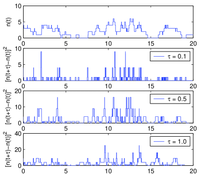
Figure 1: Simulation of the oscillator occupation number dynamics, described by Eq. (Measurement of energy eigenstates by a slow detector). The parameters of simulation are $\Gamma_{up}=1$, $\Gamma_{dn}=1.2$

The output of a detector with high SNR, $\eta_{n}\gg 1$, is proportional to $n(t)$ (QJ’s are not masked by the detector noise). Stochastic simulation of this process is shown in the top panel of Fig. 1. The switching between the plateaus corresponding to different values of $n$ occurs with the average rate $\bar{\Gamma}\sim(\Gamma_{up}+\Gamma_{dn})\bar{n}=\Gamma_{up}(\Gamma_{up}+\Gamma_{dn})/(\Gamma_{dn}-\Gamma_{up})$, where $\Gamma_{up}=\lambda_{1}^{2}\ell_{0}^{2}{\tilde{G}_{\mathcal{F}}}(\omega_{0})$ is the transition rate from the ground state into the first excited ($0\rightarrow 1$), and $\Gamma_{dn}=\lambda_{1}^{2}\ell_{0}^{2}{\tilde{G}_{\mathcal{F}}}(-\omega_{0})$ is the opposite rate ($1\rightarrow 0$), see Eq. (Measurement of energy eigenstates by a slow detector). The fast switching is superimposed on top of the slow dynamics occurring on the time scale of the inverse damping coefficient, $\gamma^{-1}=(\Gamma_{dn}-\Gamma_{up})^{-1}$.

In the presence of a detector noise the QJ may not be directly observable in $I(t)$. However, there still may be signatures in the signal correlations. First let’s consider the two-point time autocorrelation function $C_{2}(t_{1},t_{2})=\langle n(t_{1})n(t_{2})\rangle$ which enters the output autocorrelation function, $\langle I(t_{1})I(t_{2})\rangle$. It can be expressed in terms of the stationary probability distribution $P(n)$ and the conditional probability that the system is in state $n_{2}$ at time $t_{2}$ given that it was in state $n_{1}$ at an earlier time $t_{1}$, $P(n_{2},t_{2};n_{1},t_{1})$, as $C_{2}(t_{1},t_{2})=\sum_{n_{1},n_{2}}{n_{2}P(n_{2},t_{2};n_{1},t_{1})n_{1}P(n_{1})}$. From the equation of motion for $\tilde{n}(t)=\sum_{n}{n\rho_{nn}(t)}$ that can be obtained from Eq. (Measurement of energy eigenstates by a slow detector), it is easy to see, however, that $C_{2}$ is not sensitive to the fast switching with rate $\bar{\Gamma}$.

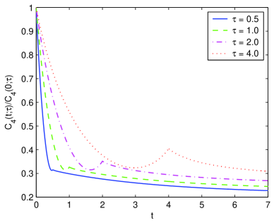
Figure 2: Four-point correlation function containing the information about fast switching between the number states. The parameters of simulation are $\Gamma_{up}=1$, $\Gamma_{dn}=1.2$

Therefore, in order to extract the signatures of the fast switching, we need to go to higher-order correlators. One approach is to convert the multi-level staircase dynamics into a two-level, or telegraph switching. This is achieved by performing the following non-linear transformation on the output signal: $I(t)\rightarrow[I(t+\tau)-I(t)]^{2}$. It will be telegraph-like if $\bar{\Gamma}\tau\ll 1$. Examples for different values of $\tau$ are shown in the lower three panels of Fig. 1. We now define the four-point correlation function,

$$C_{4}(t_{1},t_{2};\tau)=\langle[n(t_{2}+\tau)-n(t_{2})]^{2}[n(t_{1}+\tau)-n(t_{1})]^{2}\rangle,$$

which is expected to be sensitive to the fast switching. The contributions to this correlation have the general form $\langle n(t_{4})n(t_{3})n(t_{2})n(t_{1})\rangle$, with $t_{4}>t_{3}>t_{2}>t_{1}$. Similar to the two-point correlation function, it can be expressed as

$$\sum_{n_{1},n_{2},n_{3},n_{4}}n_{4}P(n_{4},t_{4};n_{3},t_{3})n_{3}P(n_{3},t_{3};n_{2},t_{2})$$ (15)

$$\times n_{2}P(n_{2},t_{2};n_{1},t_{1})n_{1}P(n_{1}).$$

Rewriting Eq. (Measurement of energy eigenstates by a slow detector) in the matrix form, $\dot{\rho}=M\rho$, the transition matrices can be expressed as

$$P(n_{2},t_{2};n_{1},t_{1})=U\exp[D(t_{2}-t_{1})]U^{-1},$$ (16)

where $D$ is a diagonal matrix of eigenvalues and $U$ is the matrix of eigenvectors of $M$, $MU=UD$. Performing numerical diagonalization on the truncated system of equations (Measurement of energy eigenstates by a slow detector), we obtain the correlator $C_{4}(t;\tau)\equiv C_{4}(t,0;\tau)$ for various values of $\tau$, as shown in Fig. 2. Indeed we find a qualitative change when the delay time $\tau$ becomes comparable to the average switching time, $\bar{\Gamma}\tau\approx 1$. For short delay times, $\bar{\Gamma}\tau\ll 1$, the correlation function rapidly decays at short times ($t<\tau$), followed by a slow exponential decay at long times. It is easy to see that in this regime, the correlation function has to be linear, $C_{4}\propto\tau-t$ for $t\leq\tau$. For long delay times, $\bar{\Gamma}\tau>1$, the correlation function is a sum of exponentials. When an additive detector noise $\xi$ with short correlation time $\tau_{\xi}<<{\bar{\Gamma}}^{-1}$ is included, the behavior of $C_{4}$ only changes at $t<\tau_{\xi}$. Thus, as far as $\tau_{\xi}<\tau$, the extrinsic noise can be effectively filtered out and $C_{4}$ can be used to detect QJ’s.

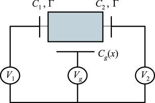
Figure 3: Scheme for SET displacement detector. Position of the oscillator modulates capacitance $C_{g}(x)$, thus modifying the current between the left and right leads.

A particular example of a measurement apparatus that can be used to perform the slow measurement described above is a Single Electron Transistor (SET). The nanoresonator interacts with the SET island via displacement-dependent gate capacitance $C_{g}(x)=C_{g}^{0}/(1-x/d)$, where $d$ is the distance between the nanoresonator and the SET island (Fig. 3). The displacement is read out by measuring the current $I$ through the SET. The island is also coupled to the leads via capacitances $C_{1}$ and $C_{2}$. For concreteness assuming that $C_{g}^{0}=C_{1}+C_{2}$, the interaction Hamiltonian is

$$H_{\rm int}=\frac{1}{2}qV_{g}\left(\frac{x}{2d}+\frac{x^{2}}{4d^{2}}\right),$$ (17)

which indeed has the form of Eq. (1), with $\mathcal{F}=q$ the island charge, $\lambda_{1}=V_{g}/(4d)$ and $\lambda_{2}=V_{g}/(8d^{2})$. To satisfy the conditions of “slow” measurement, the SET tunneling rate has to be much slower than the oscillator frequency, $\Gamma\ll\omega_{0}$. We consider the “threshold” regime, which corresponds to the resonant level nearly aligned with one of the leads’ chemical potential and corresponds to the highest read-out sensitivity. We assume that either $T\ll\Gamma$ or that SET is superconducting. Then,

$$S_{q}(0)\approx\frac{1}{\Gamma},\quad S_{q}(\omega_{0})\approx\frac{\Gamma}{\omega_{0}^{2}}.$$ (18)

SET is a nearly ideal detector set ; thus, the conditions for equality in Eq. (13) are approximately satisfied. Assuming that the intrinsic (measurement-unrelated) relaxation of the oscillator is smaller than the measurement-induced one, the signal-to-noise ratio is

$$\eta_{n}^{SET}\sim\frac{8}{(2n+1)}\times\frac{\ell_{0}^{2}}{4d^{2}}\times\frac{\omega_{0}^{2}}{\Gamma^{2}}$$ (19)

From Eqs. (8) and (14) the measurement-induced relaxation will dominate the environmental one if $\lambda_{1}^{2}\ell_{0}^{2}Q/(T\Gamma)>1$.

For a numerical estimate we take an oscillator with the frequency $\omega_{0}=2\pi\times 100$ MHz and the mass $m=2.5\cdot 10^{-17}$ (for 1$\ \mu{\rm m}\times 0.1\ \mu{\rm m}\times 0.1\ \mu{\rm m}$ dimensions at the Si density 2,500 kg/m³). The zero-point-motion amplitude is $\ell_{0}=10^{-13}$ m. Assuming that the effective separation between the nanoresonator and the SET island is $d=1$ nm and $\Gamma=10^{4}\ {\rm s^{-1}}$, for SNR we find $\eta_{n}^{SET}\sim 100/(2n+1)$. It is easy to check that the intrinsic relaxation (finite $Q$) under these conditions is insignificant compared to the SET-induced relaxation. At temperature $T=10$ mK (superconducting SET) the thermal occupation number of the resonator is about 2. Therefore, under these conditions one can expect to observe QJ between values of current that correspond to different energy eigenstates of the nanoresonator.

- (1) J. R. Friedman, V. Patel, W. Chen, S. K. Tolpygo, and J. E. Lukens, Nature 406, 43 (2000).
- (2) Y. Nakamura, Yu. A. Pashkin, and J. S. Tsai, Nature 398, 786 (1999).
- (3) J. M. Martinis, S. Nam, J. Aumentado, and C. Urbina, Phys. Rev. Lett. 89, 117901 (2002).
- (4) L. Hackermüller, S. Uttenthaler, K. Hornberger, E. Reiger, B. Brezger, A. Zeilinger, and M. Arndt, Phys. Rev. Lett. 91, 090408 (2003)
- (5) K.C. Schwab and M. L. Roukes, Physics Today, July 2005, p.36.
- (6) M. D. LaHaye, O. Buu, B. Camarota, K. C. Schwab K. Schwab, Science 304, 74 (2004).
- (7) C. M. Caves, Phys. Rev. D 26, 1817 (1982).
- (8) D. Mozyrsky and I. Martin, Phys. Rev. Lett. 89, 018301 (2002).
- (9) A. A. Clerk, Phys. Rev. B 70, 245306 (2004).
- (10) D. H. Santamore, A. C. Doherty, and M. C. Cross, Phys. Rev. B 70, 144301 (2004).
- (11) V. B. Braginsky and F. Ya. Khalili, Quantum Measurement(Cambridge Univeristy Press, Cambridge 1992).
- (12) W. H. Zurek, Rev. Mod. Phys. 75, 715 (2003).
- (13) J. P. Paz and W. H. Zurek, Phys. Rev. Lett. 82, 5181 (1999).
- (14) D. Mozyrsky, I. Martin, and M. B. Hastings, Phys. Rev. Lett. 92, 018303 (2004).