Path Integrals in the Physics of Lattice Polarons

Abstract

A path-integral approach to lattice polarons is developed. The method is based on exact analytical elimination of phonons and subsequent Monte Carlo simulation of self-interacting fermions. The analytical basis of the method is presented with emphasis on visualization of polaron effects, which path integrals provide. Numerical results on the polaron energy, mass, spectrum and density of states are given for short-range and long-range electron-phonon interactions. It is shown that certain long-range interactions significantly reduce the polaron mass, and anisotropic interactions enhance polaron anisotropy. The isotope effect on the polaron mass and spectrum is discussed. A path-integral approach to the Jahn-Teller polaron is developed. Extensions of the method to lattice bipolarons and to more complex polaron models are outlined.

1 Introduction

The polaron problem was one of the first applications of path integrals (PI). Just a few years after the introduction of the new technique into quantum mechanics Dirac1933 ; Feynman1948 and quantum statistics Kac1949 Feynman published his seminal paper Feynman1955 on the theory of Fröhlich polaron Froehlich , which set a stage for the development of polaron physics for the next half a century. The main feature of the statistical PI is an extra dimension that transforms each point-like particle into a one-dimensional line, or path. The extra dimension, to be called here the imaginary time $\tau$, extends between $0$ and $\beta=(k_{B}T)^{-1}$ where $T$ is the absolute temperature at equilibrium. As a result, a quantum-mechanical system is mapped onto a purely classical system in one extra dimension. This enables visualization of quantum-mechanical objects, which is an instructive and useful feature. The quantum mechanical properties are fully recovered by considering an ensemble of paths, each contributing its own statistical weight into the system’s partition function.

Having formulated the polaron problem in PI terms, Feynman made another key advance. He showed that if the ionic coordinates entered the model only quadratically (a free phonon field) and linearly (electron-phonon interaction in linear approximation) then the infinite-dimensional integration over ionic configurations could be performed analytically and exactly. As a result, all bosonic degrees of freedom (an infinite number of them) are eliminated in favour of just one fermionic degree of freedom. Phonons remain in the system as a retarded self-interaction of the electron. In the PI language, the statistical weight of each path is exponential in its Euclidian action and the latter contains a double integral over imaginary time as opposed to a single integral in cases of ordinary instantaneous interactions. Different segments of the fermion path “feel” each other if they are separated in imaginary time by less than the inverse phonon frequency. As a result, the electron path stiffens which leads to an enhanced effective mass and other characteristic effects as detailed later in the chapter.

The resulting electron path integral could not be calculated analytically due to the complex nature of the retarded self-interaction. Feynman resolved the difficulty by employing an original variational principle, in which the exact polaron action was replaced by an approximate, but exactly solvable, quadratic action. That led to a remarkably accurate top bound for the energy of the Fröhlich polaron (see Devreese1966 ; Prokofev1998 ; Mishchenko2000 ), which was only marginally improved by subsequent generalizations of the method Osaka1959 ; Abe ; Saitoh1980 ; Fedyanin1982 ; DeFilippis2003 . The PI method became a workhorse of the Fröhlich polaron research for decades and inspired numerous extensions which included polaron mobility Feynman1962 ; Thornber1970 ; Peeters1984 and optical conductivity Devreese2006 , polaron in a magnetic field Peeters1982 ; Devreese1992 , large bipolaron Verbist1990 , and others. Feynman’s method also inspired a Fourier Monte Carlo method, in which only the difference between the exact and variational energy was calculated numerically Alexandrou1990 ; Alexandrou1992 . Recently, the variational PI treatment was extended to a many-polaron system Brosens2005 .

In the parallel development of the small-polaron physics, Feynman’s remarkable reduction had not been utilized for almost thirty years. Although the phonon integration could be performed as well the self-interacting electron PI could not be calculated. The problem was that on the lattice even a free particle possessed a non-quadratic action. Because such a path integral could not be done analytically, it could not serve as a trial variational action. The situation changed in 1982 when De Raedt and Lagendijk (DRL) observed DeRaedt1982 that the electron PI could instead be evaluated numerically. Metropolis Monte Carlo Metropolis1953 was ideally suited for the task because the polaron action was purely real, and as such resulted in a positive-definite statistical weight of the path. Using this approach, DRL obtained a number of nice results on the Holstein polaron: confirmed formation of a self-trapped state with increasing strength of the electron-phonon interaction, observed that the crossover gets sharper with decreasing phonon frequency and increasing lattice dimensionality DeRaedt1982 , and that the critical coupling goes down as a dispersive phonon mode softens DeRaedt1984 . These results were reviewed in DeRaedt1985 . DRL also provided the first Monte Carlo analysis of the Holstein bipolaron DeRaedtBipolaron .

The works of DRL were an important step forward in the application of PI to lattice polarons. Their method could handle infinite crystal lattices of arbitrary symmetry and dimensionality, dispersive phonons, and long-range electron-phonon interactions. At the same time, it was still limited to thermodynamical properties such as energy, specific heat, and static correlation functions. In addition, it suffered from a systematic error caused by finite discretization of imaginary time (the Trotter slicing). These limitations were removed in 1997-1998. Firstly, it was shown how open boundary conditions in imaginary time could enable direct calculation of the polaron effective mass KornilovitchPike1997 and even the entire spectrum and density of states Kornilovitch1999 . The open boundary conditions allow projection of the partition function on states with definite polaron momenta. This is a particular manifestation of the general projection technique in the presence of a global symmetry. Systematic application of this principle makes it possible to separate states of different symmetries in many interesting situations, most notably bipolarons of different parity and orbital symmetry. More about the projection technique is in Section 2. Secondly, the polaron Monte Carlo method was formulated in continuous imaginary time Kornilovitch1998 , which completely eliminated the Trotter slicing and tremendously improved the computational efficiency of the method. This will be described in detail in Section 3. As a result, the versatility of DRL’s method was enhanced by better computational efficiency and by a number of new polaron and bipolaron properties that could be computed with path integrals. The method was further developed in longrange ; anisotropy ; Kornilovitch2000 ; isotope ; Spenser2005 ; Hague2005 ; multiphonon ; Hague2006 , the content of which will be described later in the Chapter.

The path-integral Quantum Monte Carlo (PIQMC) with phonon integration is only one from an impressive list of numerical methods developed for polaron models in the last three decades. There exist several other QMC techniques, in particular the path-integral QMC without phonon integration Hirsch1982 ; HirschSSH , Fourier QMC Alexandrou1990 ; Alexandrou1992 , diagrammatic QMC Prokofev1998 ; Mishchenko2000 ; Mishchenko2003 ; MishchenkoNagaosa2004 ; Macridin2004 ; Mishchenko2006 and Lang-Firsov QMC Hohenadler2004 ; Hohenadler2005 ; Hohenadler2006 . Non-QMC classes of methods include exact diagonalization Kabanov1994 ; Wellein1996 ; Wellein1997 ; Fehske2000 ; Bronold2002 ; Fehske2006 , variational calculations DeFilippis2003 ; Romero1998 ; Bonca1999 ; Bonca2000 ; Bonca2001 ; Ku2002 ; ElShawish2003 ; Cataudella2000 ; Perroni2004 ; Cataudella2006 and the density-matrix renormalization group Jeckelmann1998 ; Jeckelmann1999 ; Zhang1999 . Despite proliferation of methods, most of them have been applied to the two major polaron models: the ionic crystal model of Fröhlich Froehlich and molecular crystal model of Holstein Holstein1959 . (The notable exceptions are the Jahn-Teller (bi)polaron Kornilovitch2000 ; ElShawish2003 and Peierls instabilities HirschSSH ; Wellein1998 ; Weisse1998 .) Due to its versatility, PIQMC is uniquely positioned to study many other models, for example long-range and anisotropic electron-phonon interactions. In addition, it provides some (bi)polaron properties that are difficult to obtain by other methods such as the density of states. In this way, several physically interesting results have been obtained that include, in particular, the light polaron mass in the case of long-range electron-phonon interactions longrange , the enhancement of polaron anisotropy by electron-phonon interaction anisotropy , formation of a peak in the polaron density of states Kornilovitch1999 ; Kornilovitch2000 ; Hague2005 , the isotope effect on the polaron spectrum and density of states isotope , and the “superlight” crab-like bipolaron Alexandrov1996 ; Kornilovitch2002 ; Hague2006 . These and other results obtained by the PIQMC method in the last decade will be reviewed in Section 4. Various extensions of PIQMC and its prospects are given in Section 5.

2 Projected partition functions

It is commonly believed that the statistical path integral can provide information only on the ground state of a quantum mechanical system, and in general this is true. However, when the system possesses a global symmetry suitable projection operators can project the configurations on sectors of the Hilbert space corresponding to different irreducible representations of the symmetry group. That enables access to the lowest states within each sector and provides valuable information about system’s excitations. This strategy proves very useful in the path-integral studies of polaron models. It enables calculation of the polaron mass, spectrum, density of states, bipolaron singlet-triplet splitting and other properties. The above considerations are formalized as follows. The full thermodynamic partition function is a trace of the density matrix:

$$Z=\sum_{{\bf R}}\langle{\bf R}|e^{-\beta H}|{\bf R}\rangle\>,$$ (1)

where $H$ is the Hamiltonian and $|{\bf R}\rangle$ is a complete set of basis states in the real-space representation. If there is a global symmetry group $G$ with a set of irreducible representations $U$, it is meaningful to compose a projected partition function $G_{U}$ which is a trace over the $U$-sector of the Hilbert space only:

$$Z_{U}=\sum_{{\bf R}_{U}}\langle{\bf R}_{U}|e^{-\beta H}|{\bf R}_{U}\rangle=\sum_{\bf R}\langle{\bf R}|O^{\dagger}_{U}e^{-\beta H}O_{U}|{\bf R}\rangle\>,$$ (2)

where operator $O_{U}$ generates a basis state $|{\bf R}_{U}\rangle$ from an arbitrary state $|{\bf R}\rangle$. In the low-temperature limit $\beta\rightarrow\infty$, the partition function is dominated by the lowest $U$-eigenvalue, $Z_{U}\rightarrow\exp{(-\beta E_{U})}$. Thus $E_{U}$ can be found by taking the logarithm of $Z_{U}$ in the low-temperature limit. This is particularly efficient if the first excited state in $U$ is separated from $E_{U}$ by a finite gap.

The most important application of this technique is the formula for the (bi)polaron effective mass. In this case, irreducible representations $U$ are labeled by the total momentum ${\bf K}$ and the projection operator is $O_{\bf K}=\sum_{\bf r}e^{i{\bf K}{\bf r}}T_{\bf r}$, where $T_{\bf r}$ is the shift operator by a lattice vector ${\bf r}$. The ${\bf K}$-projected partition function is then Kornilovitch1999

$$Z_{\bf K}=\sum_{\Delta{\bf r}}e^{i{\bf K}\Delta{\bf r}}\langle{\bf R}+\Delta{\bf r}|e^{-\beta H}|{\bf R}\rangle=\sum_{\Delta{\bf r}}e^{i{\bf K}\Delta{\bf r}}Z_{\Delta{\bf r}}\>.$$ (3)

Here ${\bf R}+\Delta{\bf r}$ denotes a many-particle configuration ${\bf R}$, which is parallel-shifted as a whole by a lattice vector $\Delta{\bf r}$. The partition function $Z_{\Delta{\bf r}}$ is a “shifted trace” of the density matrix: it connects ${\bf R}$ not with ${\bf R}$ but with ${\bf R}$ shifted by $\Delta{\bf r}$. It follows from the above equation that $Z_{\bf K}$ and $Z_{\Delta{\bf r}}$ satisfy a Fourier-type relationship (for a more detailed derivation, cf. Refs. Kornilovitch1999 ; Kornilovitch2005 ). The partition function $Z_{\Delta{\bf r}}$ is formulated in real space and as such can be represented by a real-space path integral. The partition function $Z_{\bf K}$ is diagonal in momentum space and therefore contains information about the variation of system’s properties with ${\bf K}$. The Fourier theorem (3) is key to the ability to infer the (bi)polaron spectrum and mass from the path integral.

Dividing $Z_{\bf K}$ by $Z_{{\bf K}=0}$ one obtains in the zero temperature limit

$$\frac{Z_{\bf K}}{Z_{{\bf K}=0}}=e^{-\beta(E_{\bf K}-E_{0})}=\frac{\sum_{\Delta{\bf r}}e^{i{\bf K}\Delta{\bf r}}\langle{\bf R}+\Delta{\bf r}|e^{-\beta H}|{\bf R}\rangle}{\sum_{\Delta{\bf r}}\langle{\bf R}+\Delta{\bf r}|e^{-\beta H}|{\bf R}\rangle}=\langle\cos{{\bf K}\Delta{\bf r}}\rangle_{\rm shift}\>.$$ (4)

The ratio of two sums over $\Delta{\bf r}$ represents the mean value of $\exp{(i{\bf K}\Delta{\bf r})}$ over an ensemble of paths in which the two end-point many-body configurations are identical up to an arbitrary parallel shift. In the QMC language, simulations need to be performed with open boundary conditions in imaginary time. There is a certain parallel with the uncertainty principle: fixing the boundary conditions in imaginary time (by making them periodic) results in a mix of all possible momenta. Conversely, relaxing the boundary conditions by mixing in all possible shifts $\Delta{\bf r}$ allows extraction of information on the given ${\bf K}$-sector of the Hilbert space. Resolving the last equation with respect to $E_{\bf K}$, one obtains an estimator for the (bi)polaron spectrum

$$E_{\bf K}-E_{0}=-\lim_{\beta\rightarrow\infty}\frac{1}{\beta}\ln\langle\cos{{\bf K}\Delta{\bf r}}\rangle_{\rm shift}\>.$$ (5)

The left-hand-side of this equation is a constant that depends on the parameters of the model being simulated. Therefore, the average cosine on the opposite side must decrease exponentially with $\beta$ to compensate the growing denominator. At some $\beta$ it becomes too small to be measured reliably with the available statistics of a Monte Carlo run. This is an incarnation of the infamous “sign problem” that plagues many QMC algorithms. In physical terms, at very low temperatures the probability to access an excited state is exponentially low due to the Boltzmann weight factor. As a result, the QMC process samples relevant configurations exponentially rarely. These considerations put the low limit on the temperature of the simulation (high limit on $\beta$). At the same time, the condition that $Z_{\bf K}$ is dominated by a single eigenstate in the ${\bf K}$ sector, puts a high limit on temperature. Thus there is an interval of temperatures at which a meaningful calculation of (bi)polaron spectrum can be performed. If the expected bandwidth is too large the temperature interval shrinks to zero, which renders the calculation impossible. In general, the (bi)polaron spectrum can be computed by this method if the total bandwidth is smaller than the phonon frequency.

Expanding (5) for small momenta, one derives an estimator for the $\mu$-th component of the inverse effective mass

$$\frac{1}{m^{\ast}_{\mu}}=\lim_{\beta\rightarrow\infty}\frac{\langle(\Delta r_{\mu})^{2}\rangle_{\rm shift}}{\hbar^{2}\beta}\>.$$ (6)

Since in the present formulation the end points of the path are not tied together path evolution between $\tau=0$ and $\tau=\beta$ can be regarded as diffusion of the top end with respect to the bottom end over a diffusion time $\beta$. According to the Einstein relation, the mean square displacement of a diffusing particle is proportional to time. Then (6) implies that the inverse effective mass is proportional to the diffusion coefficient $D$ of the path in imaginary time KornilovitchPike1997 ; Kornilovitch1998 ; Kornilovitch2005 . The combination $\hbar\beta$ has the dimensionality of time, so the inverse mass can be written as

$$\frac{1}{m^{\ast}_{\mu}}=\frac{2D}{\hbar}\>.$$ (7)

This formula works for both polarons and bipolarons Macridin2004 ; Hague2006 . It can be viewed as a fluctuation-dissipation relation because it equates a dynamical characteristic, the mass, with an equilibrium thermodynamic property $D$. In addition, it provides a nice visualization of the main polaron effect: effective mass increase caused by an electron-phonon interaction. As will be shown in the next section, phonon integration results in correlations between distant parts of the imaginary-time polaron path. This increases the statistical weight of paths with straight segments. The average polaron path stiffens, which translates in a reduced diffusion coefficient $D$ and, according to (7), enhanced effective mass. Note that these considerations apply equally well to other types of composite particles whose mass originates from interaction. The most notable examples are defects in quantum liquids Boninsegni1995 and the hadrons of quantum chromodynamics.

Another important application of the projection technique is the singlet-triplet splitting of the bipolaron, or, more generally, of a two-fermion bound state. Coming back to the projected partition function $Z_{U}$, (2), the relevant projection operators are identified as $O_{S}=I+X$ for singlet states and $O_{T}=I-X$ for triplet states. Here $I$ is the identity operator and $X$ is the fermion exchange operator, $X|{\bf r}_{1}{\bf r}_{2}\{\xi\}\rangle=|{\bf r}_{2}{\bf r}_{1}\{\xi\}\rangle$, where $\{\xi\}$ are the ionic displacements. Upon substitution in (2) one finds

$$Z^{S,T}=\sum_{{\bf r}_{1}{\bf r}_{2}\{\xi\}}\langle{\bf r}_{1}{\bf r}_{2}\{\xi\}|e^{-\beta H}|{\bf r}_{1}{\bf r}_{2}\{\xi\}\rangle\pm\langle{\bf r}_{2}{\bf r}_{1}\{\xi\}|e^{-\beta H}|{\bf r}_{1}{\bf r}_{2}\{\xi\}\rangle\>.$$ (8)

Monte Carlo simulation proceeds over an ensemble of paths that have identical end configurations up to exchange of the top ends of the two fermion trajectories. For the singlet, both types of configurations contribute a phase factor $(+1)$ whereas for the triplet the direct paths contribute $(+1)$ and exchanged paths contribute $(-1)$. Forming the ratio of the triplet and singlet partition functions one obtains an estimator for the $S-T$ energy split

$$E^{T}_{0}-E^{S}_{0}=-\lim_{\beta\rightarrow\infty}\frac{1}{\beta}\ln\langle(-1)^{P}\rangle_{\rm ex}\>.$$ (9)

Here $(-1)^{P}=\pm 1$ for the direct and exchanged two-fermion paths. If the ends of the two paths coincide then $(-1)^{P}=0$. All said above about the sign problem and the role of temperature in calculating the average cosine applies to this expression as well.

Equation (9) provides the energy difference between the lowest triplet and singlet states. It is possible to compute the effective mass and the entire spectrum of the triplet bipolaron. To this end, one needs to combine the two symmetries considered above: the translational and exchange. This naturally leads to a path ensemble with the end configurations differing by any combination of parallel shifts and exchanges. Without repeating the derivation, the final expressions are

$$E^{T}_{\bf K}-E^{T}_{0}=-\frac{1}{\beta}\ln\left(\frac{Z^{T}_{\bf K}}{Z^{S}_{0}}\frac{Z^{S}_{0}}{Z^{T}_{0}}\right)=-\frac{1}{\beta}\ln\frac{\langle(-1)^{P}\cos({\bf K}\Delta{\bf r})\rangle_{\rm shift,ex}}{\langle(-1)^{P}\rangle_{\rm shift,ex}}\>,$$ (10)

for the triplet spectrum and

$$\frac{1}{m^{T}_{i}}=\frac{1}{\beta\hbar^{2}}\frac{\langle(-1)^{P}(\Delta r_{i})^{2}\rangle_{\rm shift,ex}}{\langle(-1)^{P}\rangle_{\rm shift,ex}}\>,$$ (11)

for the triplet mass. For the singlet spectrum and mass, (5) and (6) are still valid, except that the boundary conditions must be changed to “shift and exchange”. The same applies to the singlet-triplet estimator (9).

3 Continuous-time path-integral quantum Monte Carlo method

The main appeal of quantum Monte Carlo (QMC) methods is the ability to calculate physical properties without approximations. A quantum mechanical system is directly simulated taking into account all the details of particle dynamics and inter-particle interaction. Physically interesting observables can be calculated without bias while the statistical errors in general decrease with increasing simulation time. It is said therefore that QMC provides “numerically exact” values for the observables. A number of comprehensive reviews on QMC exist Binder1978 ; Binder1984 ; DeRaedt1985 ; Binder1995 ; Ceperley1995 ; Foulkes2001 . Many problems of the early QMC methods, such as the finite-size effects, finite time-step effects, and critical slowing down, have been resolved with the development of novel algorithms and increasing computing power. The sign problem, that is the non-positive-definiteness of the statistical weight of basis configurations, remains the only fundamental problem. In real systems and models without a sign problem (for example liquid and solid He⁴ Ceperley1995 ; Gordillo1998 ; Bauer2000 ; Ceperley2004 ; Clark2006 ), QMC works beautifully and provides with accurate and valuable information about the thermodynamics and sometimes real-time dynamics.

One polaron is free from the sign-problem difficulties. Phonons are bosons and as such do not lead to a fermion sign problem. And as long as there is only one polaron in the system statistics does not matter. This is the main reason behind the success of the QMC approach to the polaron. The ground state energy, the effective mass, isotope exponents on mass, the number of excited phonons, static correlation functions and other quantities can be calculated without any approximations. The bipolaron ground state can also be investigated without a sign problem as long as the bipolaron is a spin singlet with a symmetric spatial wave function. Thus the power of QMC can be (and has been) applied to bipolarons of various kinds and to pairs of distinguishable particles such as the exciton. For many-polaron systems the fermion sign problem fully manifests itself, which limits the applicability of QMC methods. More about this will be said in Section 5. In this Section the basics of the continuous-time path-integral quantum Monte Carlo (PIQMC) method for lattice polarons are described.

The starting point is the shift partition function $Z_{\Delta{\bf r}}$, see (3), and the electron-phonon (e-ph) Hamiltonian

$$H=-t\sum_{\bf nn^{\prime}}c^{\dagger}_{\bf n^{\prime}}c_{\bf n}-\sum_{\bf nm}f_{\bf m}({\bf n})c^{\dagger}_{\bf n^{\prime}}c_{\bf n}\xi_{\bf m}+\sum_{\bf m}\left(-\frac{\hbar^{2}}{2M}\frac{\partial^{2}}{\partial\xi^{2}_{\bf m}}+\frac{M\omega^{2}}{2}\,\xi^{2}_{\bf m}\right)\>.$$ (12)

The Hamiltonian is written in mixed representation, $c_{\bf n}$ being fermionic annihilation operators and $\xi_{\bf m}$ ion displacements. Index ${\bf n}$ denotes the spatial location of an electron Wannier orbital whereas ${\bf m}$ denotes that of an ion displacement. In general, ${\bf n}\neq{\bf m}$ even if they belong to the same lattice unit cell. For simplicity, the electron kinetic energy (the first term of $H$) is taken in the nearest-neighbor-hopping approximation with amplitude $-t$, and the lattice energy (third term in $H$) in the independent Einstein oscillator approximation with mass $M$ and frequency $\omega$. Neither approximation is necessary. Section 5 explains how PIQMC deals with more complex forms of kinetic energy and phonon spectrum. The most interesting part is the e-ph interaction (second term in $H$) which is written in the “density-displacement” form. The quantity $f_{\bf m}({\bf n})$ is the force with which an electron ${\bf n}$ acts on the ion coordinate ${\bf m}$. Asymmetric notation emphasizes that the force $f_{\bf m}$ is an attribute of a given oscillator, while the argument ${\bf n}$ is a dynamic variable indicating the current position of the electrons interacting with ${\bf m}$. No constraints are imposed on the functional form of $f$, thus allowing studies of long-range e-ph interactions. The commonly used Holstein model Holstein1959 corresponds to a localized force function $f_{\bf m}({\bf n})=\kappa\delta_{\bf nm}$.

3.1 Handling kinetic energy in continuous time

Handling the kinetic energy on a lattice possesses a challenge for Monte Carlo. To see this consider just the kinetic part of $H$ and one free particle. By introducing multiple resolutions of identity, $\hat{I}=\sum_{\bf r}|{\bf r}\rangle\langle{\bf r}|$, the shift partition function is developed into a multidimensional sum

$$Z_{\Delta{\bf r}}=\sum_{{\bf r}_{1}{\bf r}_{2}\ldots{\bf r}_{M}}\langle{\bf r}_{1}+\Delta{\bf r}|e^{-\Delta\tau H_{\rm el}}|{\bf r}_{M}\rangle\ldots\langle{\bf r}_{3}|e^{-\Delta\tau H_{\rm el}}|{\bf r}_{2}\rangle\langle{\bf r}_{2}|e^{-\Delta\tau H_{\rm el}}|{\bf r}_{1}\rangle\>,$$ (13)

where $\Delta\tau=\beta/L$ is the time step and $L+1$ is the number of time slices. Each matrix element from the product is expanded to the first power in $\Delta\tau$:

$$\langle{\bf r}_{j+1}|e^{-\Delta\tau H_{\rm el}}|{\bf r}_{j}\rangle=\delta_{{\bf r}_{j+1},{\bf r}_{j}}+t\Delta\tau\sum_{\bf l}\delta_{{\bf r}_{j+1},\,{\bf r}_{j}+{\bf l}}+{\cal O}(\Delta\tau^{2})\>,$$ (14)

where ${\bf l}$ runs over the nearest neighbors. Expanding the product, the partition function becomes a sum of a large number of terms, each of which represents a particular path of the electron in imaginary time ${\bf r}(\tau)$. The paths consist of two different building blocks: straight segments and kinks, which originate from the first and second terms in (14), respectively. On straight segments the electron position does not change, whereas each kink changes the electron coordinates by vector ${\bf l}$ depending on the kink type. The statistical weight of a path with $N_{k}$ kinks is

$$W_{N_{k}}=\underbrace{(t\Delta\tau)(t\Delta\tau)\ldots(t\Delta\tau)}_{N_{k}\;{\rm times}}=(t\Delta\tau)^{N_{k}}\>.$$ (15)

Now consider two paths, $D$ and $D^{\prime}$, that differ by $D^{\prime}$ having one extra kink of type ${\bf l}$ at imaginary time $\tau$. At small $\Delta\tau$, $D^{\prime}$ has a vanishingly small statistical weight compared to $D$. As a result, no meaningful detailed balance between individual paths with different number of kinks seems to be possible in the continuous-time limit. The resolution of this difficulty comes from the observation that there are infinitely many paths with $N_{k}+1$ kinks than with $N_{k}$ kinks. The small weight of individual path is compensated by the large number of paths. The combined weight of all paths with $N_{k}+1$ kinks is of the same order than the combined weight of all paths with $N_{k}$ kinks. Instead of detailed balance between individual paths one should seek detailed balance between path groups of similar combined weight. The paths $D$ and $D^{\prime}$ are regarded as representatives of such groups.

In accordance with the general ideas of the Metropolis Monte Carlo Metropolis1953 , one has to compose an equation that equates the transition rate from $D$ to $D^{\prime}$ to the reciprocal transition rate from $D^{\prime}$ to $D$. Both rates are products of three factors: the probability to have the original path, which is proportional to the path’s weight $W$, the probability $Q$ to propose the necessary change to the path, and the probability $P$ to accept the change. The detailed balance reads:

$$W(D)Q({\rm add}\;{\bf l}\;{\rm at}\;\tau)P(D\rightarrow D^{\prime})=W(D^{\prime})Q({\rm remove}\;{\bf l}\;{\rm at}\;\tau)P(D^{\prime}\rightarrow D)\>.$$ (16)

The probabilities to propose the addition and removal of the kink turn out to be two quite different quantities. In the direction $D^{\prime}\rightarrow D$, the kink to be removed is chosen from a finite number of all other kinks. Therefore the probability that it is selected for removal is a finite number $Q_{\rm remove}({\bf l};\tau)$. In contrast, in going from $D$ to $D^{\prime}$ the kink does not yet exist and the probability to propose its creation exactly at time $\tau$ is proportional to the time interval $\Delta\tau$. The probability to propose the kink’s addition is an infinitesimal quantity: $Q({\rm add}\;{\bf l}\;{\rm at}\;\tau)=q_{\rm add}({\bf l};\tau)(\Delta\tau)$, where $q_{\rm add}$ is the corresponding probability density. Substitution of these two results in the balance equation yields

$$(t\Delta\tau)^{N_{k}}q_{\rm add}({\bf l};\tau)(\Delta\tau)P(D\rightarrow D^{\prime})=(t\Delta\tau)^{N_{k}+1}Q_{\rm remove}({\bf l};\tau)P(D^{\prime}\rightarrow D)\>.$$ (17)

The extra $(\Delta\tau)$ from the addition probability on the left side exactly balances the smaller weight of the right side. The time step cancels out of the equation leaving only finite factors which are well defined in the continuous-time limit. According to the standard Metropolis recipe the solution is given by the following acceptance rules

$$P(D\rightarrow D^{\prime})=\min\left\{1\;;\;\frac{t\cdot Q_{\rm remove}({\bf l};\tau)}{q_{\rm add}({\bf l};\tau)}\right\}\>,$$ (18)

$$P(D^{\prime}\rightarrow D)=\min\left\{1\;;\;\frac{q_{\rm add}({\bf l};\tau)}{t\cdot Q_{\rm remove}({\bf l};\tau)}\right\}\>.$$ (19)

These expressions still leave a lot of freedom in specifying functions $q_{\rm add}$ and $Q_{\rm remove}$. As an example, consider the simplest choice when both functions are constant. For the addition process this means that the time for the new kink of type ${\bf l}$, on top of the existing $N_{\bf l}$, is chosen with equal probability within the $[0,\beta]$ time interval, hence ${q_{\rm add}({\bf l};\tau)}=\beta^{-1}$. For the removal process, the candidate kink for elimination is chosen from the existing $N_{\bf l}$ with equal probability, that is $Q_{\rm remove}({\bf l};\tau)=N^{-1}_{\bf l}$. One must also take into account the fact that kinks can only be added to the path if $N_{\bf l}=0$, while added or removed if $N_{\bf l}\geq 1$. The full set of update rules could be as follows. (i) Select the kink type ${\bf l}$, that is the hopping direction of the particle. The probability with which different ${\bf l}$ are selected may not be equal but must be non-zero. (ii) If the current path already has kinks of type ${\bf l}$, whether to add or remove a kink is proposed with, for example, equal probability of $\frac{1}{2}$. If the path possesses no kinks, addition is the only option, and it must be chosen with probability $1$. (iii) If addition is selected, the time for the new kink is chosen with probability density $\frac{1}{\beta}$. The update is accepted with probability $\min\{1;(t\beta)/(N_{\bf l}+1)\}$ for $N_{\bf l}\geq 1$ and with probability $\min\{1;(t\beta)/2\}$ for $N_{\bf l}=1$. (iv) If removal is selected, the candidate kink is chosen with equal probability from the existing $N_{\bf l}$. The update is accepted with probability $\min\{1;N_{\bf l}/(t\beta)\}$ for $N_{\bf l}\geq 2$ and with probability $\min\{1;2/(t\beta)\}$ for $N_{\bf l}=1$.

The described method can be readily generalized to next-nearest neighbor hopping and anisotropic hopping. It can also be generalized to multi-kink updates, as needed for example in simulating the bipolaron. To close this section one should note that a path can be interpreted as a time-space diagram, where kinks play the role of vertices and straight segments the role of propagators. Integration over the ensemble of fluctuating paths can then be understood within the general concept of Diagrammatic Monte Carlo Prokofev1998 ; ProkofevDMC .

3.2 Integration over phonons

Analytic integration over phonons is a key ingredient of the polaron PIQMC method. Although an electron-phonon (e-ph) system can be simulated without phonon integration Hirsch1982 ; HirschSSH , it is the integration that makes the method powerful. Indeed, the integration reduces $N+1$ degrees of freedom to just one degree of freedom, which increases accuracy and reduces simulation time. The integration effectively eliminates all the distant parts of the system by folding the infinite number of ion coordinates into one retarded self-interaction function. The simulation then proceeds on an infinite lattice with no finite-size effects. In addition, the integration makes it possible to simulate long-range e-ph interactions with the same efficiency as local interactions, which extends QMC capabilities towards more realistic models.

Technical details of the phonon integration are somewhat cumbersome but well-documented in the literature. Here we will describe the main steps of the derivation and point out associated subtleties.

Upon insertion of $H$ into (3), a path-integral representation for $Z_{\Delta{\bf r}}$ is developed by introducing $L$ time intervals and $L-1$ intermediate sets of basis states. In the continuous time limit, $L\rightarrow\infty$, the kinetic energy of the electron is treated as described in the previous section. Integration over the electron coordinates is converted to stochastic summation over an ensemble of paths which are sampled by adding and removing kinks. For each electron path, there is an internal path integration over the ionic coordinates characterized by the electron-phonon action $A_{\rm e-ph}$

$$Z_{\Delta{\bf r}}=\int^{({\bf r}+\Delta{\bf r},\beta)}_{({\bf r},0)}{\cal D}{\bf r}(\tau)\int^{(\{\xi_{{\bf m}-\Delta{\bf r}}\},\beta)}_{(\{\xi_{\bf m}\},0)}{\cal D}\xi_{\bf m}(\tau)\>e^{A_{\rm e-ph}[\,{\bf r}(\tau),\,\xi_{\bf m}(\tau)]}\>,$$ (20)

$$A_{\rm e-ph}=-\sum_{\bf m}\!\!\int^{\beta}_{0}\!\left[\frac{M{\dot{\xi}}^{2}_{\bf m}(\tau)}{2\hbar^{2}}+\frac{M\omega^{2}}{2}\xi^{2}_{\bf m}(\tau)\right]{\rm d}\tau+\sum_{\bf m}\int^{\beta}_{0}\!\!\!f_{\bf m}[{\bf r}(\tau)]\xi_{\bf m}(\tau){\rm d}\tau\>.$$ (21)

The path integral over $\xi_{\bf m}(\tau)$ is Gaussian and therefore can be calculated analytically. Actually, the integration is performed in two steps. Firstly, path integration is done with fixed but arbitrary boundary conditions at the two ends of the path. Secondly, a certain relationship between $\xi_{\bf m}(0)$ and $\xi_{\bf m}(\beta)$ is assumed followed by an additional one-dimensional ordinary (but still Gaussian) integration. In most PI studies, periodic boundary conditions $\xi_{\bf m}(\beta)=\xi_{\bf m}(0)$ are assumed. This leads to the classic Feynman formula for the oscillator action in the presence of an arbitrary time-dependent external force Feynman1972 . However, we have seen in the previous section that mass and spectrum calculation requires a partition function with the end configurations parallel-shifted with respect to each other. The shift of the ionic configuration must be the same as that of the fermion configuration, which implies $\xi_{\bf m}(\beta)=\xi_{{\bf m}-\Delta{\bf r}}(0)$, as indicated in the last equation. The correlation between the electron and phonon boundary conditions is illustrated in Fig. 1(a).

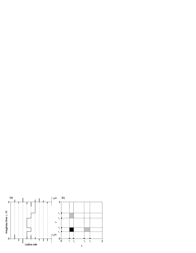
Figure 1: (a) Integration over ionic paths under shifted boundary conditions. Ionic displacements are shown as vertical bars at $\tau=0$ and $\tau=\beta$. Notice how the pattern of displacements is correlated with the shift of the electron path. The end displacements of individual oscillators are not equal, $\xi_{\bf m}(0)\neq\xi_{\bf m}(\beta)$. (b) Calculation of the polaron action as a double integral over imaginary time. The kink times $\tau_{i}$ break the $(\tau\tau^{\prime})$ plane into a finite number of rectangles. Within each rectangle the electron coordinates are constant and the double integral can be calculated analytically for arbitrary $\tau_{i}$ Spenser2005 . After that the double integral reduces to a sum over the rectangles. Since the number of rectangles decreases at strong coupling, the algorithm gets faster at strong coupling.

Due to an additional shift, the second-phase integration results in a correction to the conventional “periodic” action. The full polaron action, upon summation over all oscillators, reads Kornilovitch1998 ; multiphonon

$$A_{\rm pol}[{\bf r}(\tau)]=A_{0}+\Delta A\>,$$ (22)

$$A_{0}=\sum_{\bf m}\frac{\hbar}{4\omega M}\int^{\beta}_{0}\!\!\!\int^{\beta}_{0}{\rm d}\tau{\rm d}\tau^{\prime}\frac{\cosh\hbar\omega(\frac{\beta}{2}-|\tau-\tau^{\prime}|)}{\sinh\hbar\omega\frac{\beta}{2}}f_{\bf m}[{\bf r}(\tau)]f_{\bf m}[{\bf r}(\tau^{\prime})]\>,$$ (23)

$$\Delta A=\sum_{\bf m}\frac{\hbar}{2\omega M}B_{\bf m}\left(C_{{\bf m}+\Delta{\bf r}}-C_{\bf m}\right)\>,$$ (24)

$$B_{\bf m}\equiv\int^{\beta}_{0}{\rm d}\tau^{\prime}\frac{\sinh\hbar\omega(\beta-\tau^{\prime})}{\sinh\hbar\omega\beta}f_{\bf m}[{\bf r}(\tau^{\prime})]\>,$$ (25)

$$C_{\bf m}\equiv\int^{\beta}_{0}{\rm d}\tau^{\prime}\frac{\sinh\hbar\omega\tau^{\prime}}{\sinh\hbar\omega\beta}f_{\bf m}[{\bf r}(\tau^{\prime})]\>.$$ (26)

The polaron action is a functional of the electron path and contains all the information about the ionic subsystem. The denominator of (4) finally becomes

$$Z_{{\bf K}=0}=\sum_{\Delta\tau}Z_{\Delta{\bf r}}=Z_{\rm ph}\sum^{\infty}_{N_{k}=0,1,\ldots}\int^{\beta}_{0}\cdots\int^{\beta}_{0}({\rm d}\tau)^{N_{k}}\,t^{N_{k}}\,e^{A_{\rm pol}[\,{\bf r}(\tau)]}\>.$$ (27)

Here $Z_{\rm ph}=[2\sinh(\frac{1}{2}\hbar\beta\omega)]^{-N}$ ($N$ is the number of lattice sites) is the partition function of free phonons. It is a multiplicative constant that cancels out from all statistical averages. The factor $e^{A_{\rm pol}}$ adds to the weight of each path on top of the “kinetic” contribution $(t\Delta\tau)^{N_{k}}$. As a result, the acceptance rules (18) and (19) are modified by the ratio of the respective factors for the paths $D$ and $D^{\prime}$

$$P(D\rightarrow D^{\prime})=\min\left\{1\;;\;\frac{t\cdot Q_{\rm remove}({\bf l};\tau)}{q_{\rm add}({\bf l};\tau)}\>e^{A_{\rm pol}(D^{\prime})-A_{\rm pol}(D)}\right\}\>,$$ (28)

$$P(D^{\prime}\rightarrow D)=\min\left\{1\;;\;\frac{q_{\rm add}({\bf l};\tau)}{t\cdot Q_{\rm remove}({\bf l};\tau)}\>e^{A_{\rm pol}(D)-A_{\rm pol}(D^{\prime})}\right\}\>.$$ (29)

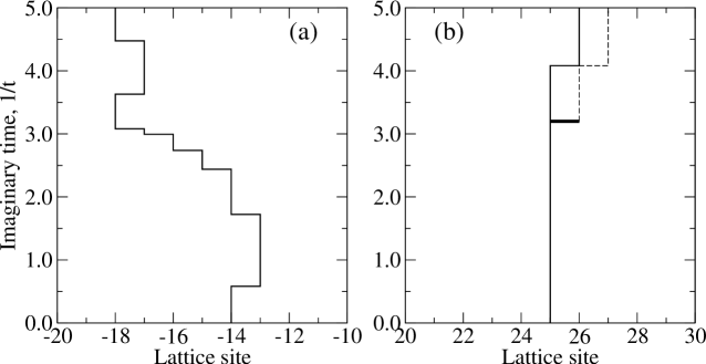
Figure 2: (a) A typical fluctuating path of a free particle on a one-dimensional chain ($E_{0}=-2.00\,t$, $m^{\ast}/m_{0}=1$). The path has drifted to the left by four lattice sites, which contributes to the effective mass according to (6). (b) A typical path of a one-dimensional Holstein polaron at $\hbar\omega/t=2.0$ and $\lambda=2.0$ ($E_{0}=-4.66(2)\,t$, $m^{\ast}/m_{0}=3.06(3)$. The path has drifted to the right by just one site reflecting a larger mass. The thick bar is a kink update proposed by Monte Carlo. If accepted, the top part of the path is changed to the dashed line (top shift). Alternatively, the bottom part of the path can be shifted by one site to the left (bottom shift).

These acceptance rules together with the formula for the polaron action and path update rules described in the previous section fully define the Monte Carlo update process. It is illustrated in Fig. 2. Numerical efficiency of the algorithm critically depends on how easily the polaron action can be computed at every update. The task is greatly aided by the fact that the electron path is defined on a discrete lattice. In other words, it consists of a finite number of straight segments. This has two important consequences. First, because within each segment the electron coordinate is independent of imaginary time $\tau$, the forces $f_{\bf m}({\bf r})$ can be taken outside the time integration. The rest of the integrand is an explicit function of $\tau$ and $\tau^{\prime}$. This time integral can be calculated analytically for arbitrary end times of the segment. The double integral over time becomes a double sum over the segments, as illustrated in Fig. 1(b). The summand is a simple function of kink times; the explicit expressions are given in Spenser2005 . The smaller the number of segments, that is the straighter the path, the less time is required to compute $A_{\rm pol}$. The electron-phonon interaction increases the statistical weight of straight paths and reduces the mean number of segments. Thus, in contrast to most other numerical methods, PIQMC becomes faster at large electron-phonon couplings.

Secondly, the $(ij)$-th term of the sum over segments contains the electron-ion forces in the combination

$$\Phi({\bf r}_{i}-{\bf r}_{j})=\sum_{\bf m}f_{\bf m}({\bf r}_{i})f_{\bf m}({\bf r}_{j})\>,$$ (30)

where ${\bf r}_{i}$ is the electron coordinate on $i$-th segment. The coefficients $\Phi$ are defined on a discrete set of points and can be pre-computed for a sufficiently large range of coordinate separation. After that the simulation takes essentially the same amount of time for any form of electron-phonon interaction. This is why the PIQMC polaron method is as efficient for long-range e-ph interactions as for the short-range Holstein model.

We close this section by noting that the requirement of phonon integration with shifted boundary conditions equally applies to the continuous case. This does not seem to be the case with the original Feynman’s calculation of the mass of the Fröhlich polaron and its subsequent generalizations. This issue was thoroughly investigated in KornilovitchFeynman2005 . It was shown that the periodic boundary conditions in the phonon integration, while absolutely correct for the energy calculation, lead to infinite terms in the polaron action in the mass calculation. Feynman’s mass formula is obtained only if the terms are regarded as unphysical and thrown out by hand. In contrast, the shifted boundary conditions result in a self-consistent action and Feynman result is obtained without any complications.

3.3 Observables

The preceding sections explained how to organize an efficient Monte Carlo sampling process that simulates the electron kinetic energy while fully taking into account the ion dynamics and electron-phonon interaction. Note that no approximation has been made so far except for the quadratic form of the elastic energy of the crystal. In this section it will be explained how to extract useful physical information from the one-to-one correspondence between the quantum mechanical-polaron and an ensemble of self-interacting paths. A number of important estimators have already been derived in Section 2. In particular, the effective mass is obtained from the mean-square end-to-end distribution, see (6). The polaron spectrum relative to the ground state is given by (5). It is essential that statistics for different $E_{\bf K}$ is collected in parallel so that the entire polaron spectrum is obtained in a single run. One consequence of this remarkable property is PIQMC’s ability to compute the polaron density of states by simply histogramming $E_{\bf K}$ at the end. At present, PIQMC is the only method capable of efficiently calculating the polaron density of states.

The next important characteristic is the absolute polaron energy $E_{0}$. One way to obtain $E_{0}$ is from the low-temperature limit of the internal energy $U$. The latter can be computed from the thermodynamic relation $U=-\partial\ln Z/\partial\beta$. Since we are interested in the ground state, the corresponding partition function must be $Z_{{\bf K}=0}=\sum_{\Delta{\bf r}}Z_{\Delta{\bf r}}=\sum_{\rm shifted\>paths}W[{\bf r}(\tau)]$. Returning momentarily to discrete time, $\beta=L\Delta\tau$,

$$U=-\frac{1}{L}\frac{\sum_{\rm shift}\frac{\partial W}{\partial\Delta\tau}}{\sum_{\rm shift}W}=-\frac{1}{L}\frac{\sum_{\rm shift}\left[\frac{1}{W}\frac{\partial W}{\partial\Delta\tau}\right]W}{\sum_{\rm shift}W}=-\frac{1}{M}\left\langle\frac{1}{W}\frac{\partial W}{\partial\Delta\tau}\right\rangle_{\rm shift}.$$ (31)

The weight $W$ is a product of the kinetic contribution $(t\Delta\tau)^{N_{k}}$ and the phonon term $e^{A_{\rm pol}}$. Substituting in the above expression, one obtains a ground-state energy estimator

$$E_{0}=-\frac{1}{L}\left\langle\frac{N_{k}}{\Delta\tau}+\frac{\partial A_{\rm pol}}{\partial\Delta\tau}\right\rangle_{\rm shift}=\left\langle-\frac{N_{k}}{\beta}-\frac{\partial A_{\rm pol}}{\partial\beta}\right\rangle_{\rm shift}.$$ (32)

The two terms here represent the kinetic and potential energy of the polaron, respectively. The kinetic energy is simply the mean number of kinks on the path. One can regard the kinks as “quanta” of the kinetic energy, each contributing the same amount $-\beta^{-1}$. With increasing coupling the paths become “stiffer”, that is the mean number of kinks goes down. As a result, the polaron kinetic energy decreases by absolute value. Measuring the potential energy is harder for it is derived from the polaron action. Similarly to the latter, the potential energy estimator can be reduced to a double sum over the path’s segments. Explicit expressions for the double sum terms are given in Spenser2005 .

The number of excited phonons $N_{\rm ph}$ in the polaron cloud is another interesting characteristic. It measures the amount of energy stored in the lattice deformation around the electron. The polaron mass scales exponentially with $N_{\rm ph}$ so in addition the latter gives a rough estimate of the polaron mass. An estimator for $N_{\rm ph}$ can be derived by noting that the last term in the Hamiltonian (12) can be rewritten as $\hbar\omega(\hat{N}_{\rm ph}+\frac{1}{2})$, where $\hat{N}_{\rm ph}$ is the operator of the total number of phonons. The mean value of $\hat{N}_{\rm ph}$ is obtained by differentiating the free energy with respect to $\hbar\omega$. To make sure that no contribution is received from the interaction term, the derivative must be taken with the combination $f^{2}/(M\omega)$ kept constant. Using $F=-\frac{1}{\beta}\ln Z$, the estimator is obtained as follows

$$N_{\rm ph}=-\frac{1}{\beta}\left.\frac{\partial F}{\partial(\hbar\omega)}\right|_{\frac{f^{2}}{M\omega}}=-\frac{1}{\beta}\left\langle\left.\frac{\partial A_{\rm pol}}{\partial(\hbar\omega)}\right|_{\frac{f^{2}}{M\omega}}\right\rangle_{\rm shift}.$$ (33)

The subscript “shift” implies that the number of phonons corresponds to the ground state of the polaron (${\bf K}=0$). It is also possible to derive estimators for non-zero total momenta, which is omitted here.

Finally, one can derive an estimator for the isotope exponent of the polaron effective mass $\alpha_{\mu}$. In the (bi)polaron mechanism of superconductivity, $\alpha_{\mu}$ is related to the isotope effect on the critical temperature Alexandrov1992 . The mass isotope exponent is defined as $m^{\ast}_{\mu}=M^{\alpha_{\mu}}$, where $M$ is the ion mass. Since the present method calculates the inverse polaron mass, $\alpha_{\mu}$ is more conveniently expressed via the inverse effective mass

$$\alpha_{\mu}=-\frac{M}{\frac{1}{m^{\ast}_{\mu}}}\frac{\partial}{\partial M}\left(\frac{1}{m^{\ast}_{\mu}}\right)=\frac{\omega}{2\left(\frac{1}{m^{\ast}_{\mu}}\right)}\frac{\partial}{\partial\omega}\left(\frac{1}{m^{\ast}_{\mu}}\right).$$ (34)

The last transformation follows from the scaling $M\propto\omega^{-2}$. The estimator for $\alpha_{\mu}$ is derived directly from the estimator for the inverse effective mass (6). A path’s weight depends on the phonon frequency only via the polaron action $e^{A_{\rm pol}}$. (One should recall that the definition of a Monte Carlo average $\langle(\Delta r_{\mu})^{2}\rangle$ contains $A_{\rm pol}$ in the numerator and denominator.) Upon differentiation one obtains

$$\alpha_{\mu}=\frac{\omega}{2\langle(\Delta r_{\mu})^{2}\rangle}\left[\left\langle(\Delta r_{\mu})^{2}\left.\frac{\partial A_{\rm pol}}{\partial\omega}\right|_{M\omega^{2}}\right\rangle-\langle(\Delta r_{\mu})^{2}\rangle\left\langle\left.\frac{\partial A_{\rm pol}}{\partial\omega}\right|_{M\omega^{2}}\right\rangle\right].$$ (35)

In taking the frequency derivative, one should keep the combination $M\omega^{2}$ constant, as it is independent of the ion mass. As with the phonon action and potential energy, the estimators for the number of phonons and isotope exponent can be split into a double sum over path’s segments. The expressions for the respective summands can be found in Spenser2005 .

4 Polaron properties

The focus of this section is going to be the polaron properties that have been obtained with the continuous-time path-integral Quantum Monte Carlo method. For each topic, additional details of the algorithm will be provided, if necessary, on top of the general description presented above.

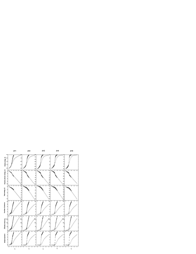
Figure 3: Properties of the Holstein polaron on $d=1,2,3,4,6$ hypercubic lattices. The filled and open symbols show data for the phonon frequencies $\hbar\omega/t=0.4$ and 1.0 ($d=1$), 0.8 and 2.0 ($d=2$), 1.2 and 3.0 ($d=3$), 1.6 and 4.0 ($d=4$), and 2.4 and 6.0 ($d=6$), respectively. The coupling constant is defined as $\lambda=E_{p}/(zt)=\kappa^{2}/(2M\omega^{2}zt)$, where $z=2d$ is the number of nearest neighbours. The effective mass is measured in units of $m_{0}=\hbar^{2}/(2ta^{2})$. Note that because the phonon frequency increases with $d$, the curves in different dimensions have similar shapes except for small differences around the $\lambda$ of polaron formation.

4.1 Long-range interaction produces light polarons

The Holstein model Holstein1959 describes polarons in systems with well-screened short-range electron-phonon interaction, such as molecular crystals. It is in the short list of “main” polaron models. Due to its simplicity, the model has been extremely popular with the numerical community. Almost any new numerical method was first tried on the Holstein model, for which a lot of accurate results are available. Also, for a long time the Holstein model was regarded as a “generic” model for all narrow-band systems where the e-ph and lattice effects were equally important. The locality of the interaction was considered simply a matter of convenience, and the Holstein model itself was believed to contain all the qualitative features of lattice polarons. This turns out not to be the case. The main reason lies in the very sharp, exponential, dependence on the model parameters of the main polaron characteristic, the effective mass. Some properties of the Holstein polaron are presented in Fig. 3. Any approximation or model simplification that have little effect on the polaron energy can have dramatic consequences for the mass, leading to false qualitative conclusions. In particular, the Holstein model is not adequate for complex oxides of transition metals such as the cuprates or manganites. In those materials the bare bands are narrow, $\sim 1-2$ eV, so the lattice effects are important. At the same time, a low density of free carriers cannot fully screen the Coulomb interaction between electrons and distant anions and cations, leading to a long-range e-ph interaction.

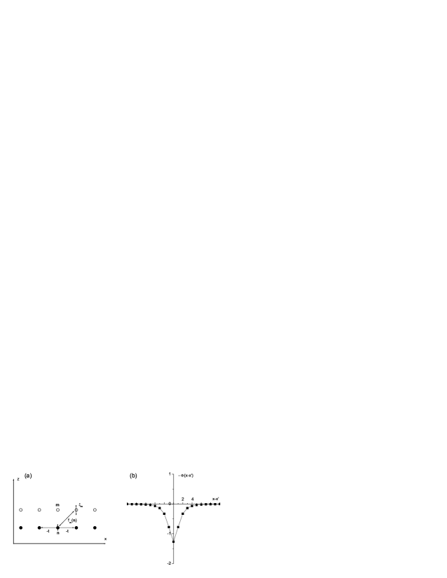
Figure 4: (a) One-dimensional model with a long-range electron-phonon interaction. The electron moves along the bottom chain of sites shown by full circles (denoted by ${\bf n}$). The vibrating ions shown by open circles oscillate along the $z$-axis. The interaction is characterized by the $z$-projection of the Coulombic force (36). (b) Spatial profile of function $\Phi$, (30), that characterizes the retarded interaction of different parts of the polaron path. The parameters are $\kappa=1$ and $d=a$. Negative $\Phi$ is shown in order to draw analogy with a potential well. This shape of $\Phi$ should be contrasted with that of the Holstein model $\Phi_{\rm Hol}=\kappa^{2}\delta_{xx^{\prime}}$. A smooth $\Phi$ cannot localize the path as well as a sharp one, which results in a smaller effective mass in the case of a long-range model.

A model of this kind was considered a long time ago by Eagles Eagles . (The corresponding polaron was called there a “nearly-small polaron”.) More recently, a long-range model with linearly polarized phonons was put forward in relation to high-temperature superconductors in longrange . The model is depicted in Fig. 4(a). An electron hops within a rigid chain (in the one-dimensional case) or plane (in the two-dimensional case) and interacts with ions that are positioned above the electron chain (or plane) and vibrate perpendicular to the chain (plane). Such a polarization was chosen to represent the $c$-polarized phonon modes that feature prominently in the cuprates Timusk1995 . The force function was taken to be the Coulomb force projected on the $z$-axis

$$f_{\bf m}({\bf n})=\kappa a^{2}\frac{({\bf n}-{\bf m})_{z}}{|{\bf n}-{\bf m}|^{3}}=\frac{\kappa a^{2}d}{[({\bf n}-{\bf n}_{\bf m})^{2}+d^{2}]^{3/2}}\>.$$ (36)

Here $a$ is the lattice constant, $d$ is the distance between the vibrating ions and the electron plane, and ${\bf n}_{\bf m}$ is the vector of the electron Wannier orbital in the same unit cell as ion ${\bf m}$. The interaction strength is characterized by the parameter $\kappa$. Alternatively, one can use a dimensionless parameter

$$\lambda=\frac{E_{p}}{zt}=\frac{1}{2M\omega^{2}zt}\sum_{\bf m}f^{2}_{\bf m}(0)\>,$$ (37)

which is a ratio of the polaron energy in the atomic limit $E_{p}$ (at $t=0$) to the kinetic energy of a free electron $zt$ (at $\kappa=0$). Here $z$ is the number of nearest lattice sites. The confinement of the polaron path is determined by the function $\Phi$, (30), whose profile is shown in Fig. 4(b). (It should be compared with the Holstein confining function $\kappa^{2}\delta_{\bf nn^{\prime}}$.) Due to loose confinement, the polaron path diffused farther than in the Holstein case, which is equivalent to a much lighter mass. Such a polaron was named the “small Fröhlich polaron” (SFP) in longrange .

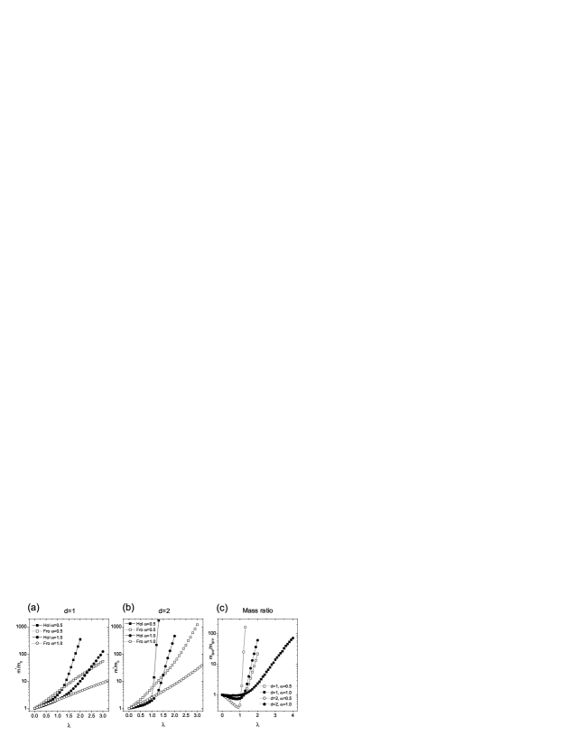
Figure 5: Effective masses of small Holstein and Fröhlich polarons in units of $m_{0}=\hbar^{2}/(2ta^{2})$. (a) $d=1$. (b) $d=2$. (c) The mass ratio of the small Holstein and Fröhlich polarons for several model parameters. The ratio scales exponentially with the coupling, and could exceed 100.

The masses of SFP and SHP calculated with PIQMC are compared in Fig. 5. SFP is slightly heavier at small $\lambda$ but much lighter at large $\lambda$. The ratio of the two masses is a non-monotonic function. This observation was later confirmed by exact diagonalization Fehske2000 and variational Bonca2001 ; Perroni2004 methods. The most interesting property of SFP is exponential reduction of mass relative to SHP, see Fig. 5(c). This effect is independent of the dimensionality because it originates solely from the long-ranginess of e-ph interaction. The mass reduction can be very large. For example, in two dimensions at $\hbar\omega/t=0.5$ and $\lambda=1.2$, $m_{\rm SHP}\approx 220$ while $m_{\rm SFP}$ is only $\approx 9$. In Spenser2005 , an additional screening factor was added to the force function (36). All polaron properties smoothly interpolated between those of SHP and SFP as the screening radius was changed from zero to infinity.

The physical reason for the small mass of SFP is easy to understand. The mass is determined by the overlap of the ionic wave functions before and after the electron hop. In the case of short-range e-ph interaction, the lattice deformation must relax all the way back to the equilibrium state after the electron leaves the site. Likewise, the lattice deformation at the new electron’s location must form anew from the equilibrium state. As a result, the overlap integral is exponentially small. In the case of a long-range interaction, the deformation at the new location is partially pre-existent. The ions must move by a smaller distance, which results in a much larger overlap of the wave functions. That also produces an exponentially large mass, but with a smaller exponent. (The fact that the mass is still exponential in coupling justifies the term “small” in the polaron’s name.) This effect can also be understood within the Lang-Firsov (LF) approximation for the polaron mass Tjablikov1952 ; Firsov1962 that becomes exact in the limit of infinitely fast ions, $\hbar\omega\gg t$. According to LF, the polaron mass is given by $m^{\ast}=m_{0}\,e^{\gamma(E_{p}/\hbar\omega)}$, where $E_{p}$ is the polaron shift from (37). The dimensionless parameter

$$\gamma=1-\frac{\sum_{\bf m}f_{\bf m}(0)f_{\bf m}({\bf a})}{\sum_{\bf m}f^{2}_{\bf m}(0)}\>,$$ (38)

depends on the shape of the e-ph interaction. For the force function (36) at $d=a$, $\gamma=0.387$ for the linear chain, $0.334$ for the square lattice and $0.320$ for the triangular lattice. Note also that a long-range e-ph interaction smoothens the polaron crossover, cf. Fig. 5, which makes the single exponential form be more applicable for the entire coupling range longrange .

These results demonstrate that the Holstein model is an extreme model that predicts the largest mass for the given polaron energy. As such, the Holstein model is not adequate for ionic systems with poor screening where the e-ph interaction is long range.

4.2 Enhancement of anisotropy by electron-phonon interaction

Two different behaviours of the lattice polaron can lead to an interesting situation when the same particle is Holstein-like and Fröhlich-like along two different lattice directions. A concrete model that features such properties was put forward in anisotropy . The model is an extension of the force function (36) to three dimensions, see Fig. 6(a). Clearly, the e-ph interaction is anisotropic, which translates to an even higher anisotropy of polaron spectrum. Upon hops along the $z$ direction, the electron must reverse the sign of deformation. Thus the ion overlap integrals are even smaller than in the Holstein case. In contrast, the movement in the $xy$ plane is Fröhlich-like, as described in the previous section. The deformation is partially prepared, the overlap integrals are large, and the effective mass is small. This reasoning is corroborated by the spatial profiles of the path confinement function $\Phi$, see Fig. 6(b). When the path diffuses along the $x$ direction, $\Phi$ is smooth which translates into easy “escape”. Along the $z$ direction, $\Phi$ is much steeper. In fact it even changes sign upon migration to the nearest plane, which reflects the sign reversal of the lattice deformation after the electron hop. Since $\Phi$ affects the path’s weight exponentially, one expects exponentially large difference between the polaron masses in $z$ and $x$ direction: $m^{\ast}_{z}/m^{\ast}_{x}\propto e^{(\gamma_{z}-\gamma_{x})\lambda/\bar{\omega}}$, where $\lambda=2.93\kappa^{2}/(12M\omega^{2}t_{x})$ and $\bar{\omega}=\hbar\omega/t_{x}$ is the dimensionless phonon frequency. As a result, the mass anisotropy grows exponentially with $\lambda$ and can reach very big values. In addition, the mass anisotropy is a sharp function of the phonon frequency, which should lead, for example, to an isotope effect on anisotropy.

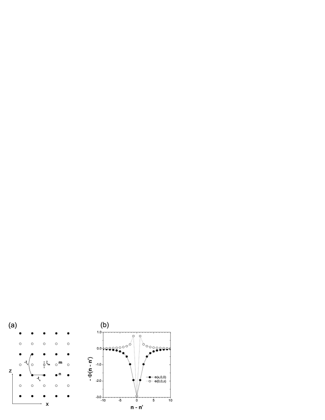
Figure 6: (a) A three-dimensional polaron model with anisotropic e-ph interaction. The electron moves within and between the planes of filled circles with hopping integrals $-t_{x}$ and $-t_{z}$, respectively. It interacts with vibrating ions shown by open circles. The vibrations are polarized along the $z$-axis. In the case of a long-range interaction the polaron is Fröhlich-like in the $xy$ plane and Holstein-like along the $z$ direction. (b) The (negative) polaron path confinement function $-\kappa^{-2}\Phi(x,y,z)$. An additional factor $e^{-{|{\bf n}-{\bf m}|}/R}$ with $R=10$ lattice constants in the $x$ direction, has been added to the force function (36) to help the lattice sum to converge. The confining profile along $z$ is much steeper than along $x$.

The results of PIQMC analysis of the model are summarized in Fig. 7 anisotropy . The inset shows a typical behaviour of the polaron masses at $\hbar\omega=1.0\,t_{x}$ and $t_{z}=0.25\,t_{x}$. (This choice of hoppings ensures the isotropy of the bare spectrum, since the lattice constant in $z$ direction is assumed to be twice the one in $x$ direction.) As expected, $m^{\ast}_{x}$ grows exponentially with coupling. Interestingly, the $z$ mass grows super-exponentially with a large quadratic component: $m^{\ast}_{z}\approx m_{x0}\,e^{1.26\lambda+0.88\lambda^{2}}$. It is very possible though that this is still transient regime, and $m^{\ast}_{z}$ approaches pure exponential growth at still larger $\lambda$ (at which $m_{z}$ becomes so large it is difficult to calculate). The mass anisotropy for several sets of model parameters is shown in the main panel of Fig. 7. Due to the super-exponential growth of $m^{\ast}_{z}$, the anisotropy is also super-exponential, e.g. $m^{\ast}_{z}/m^{\ast}_{xy}\approx e^{0.42\lambda+0.71\lambda^{2}}$ for $\hbar\omega=1.0\,t_{x}$ (circles). At a smaller frequency $\hbar\omega=0.5\,t_{x}$ (squares) the anisotropy is exponentially larger, as expected from the reasoning given above. This implies the existence of an isotope effect on the mass anisotropy. The third model parameter, the bare hopping anisotropy, turns out to have little effect on the anisotropy of the polaron spectrum. The mass anisotropy for $t_{z}=0.1\,t_{x}$ and the same phonon frequency $\hbar\omega=0.5\,t_{x}$ is shown by triangles in Fig. 7. While being $2.0-2.5$ times larger at small $\lambda$, the anisotropy approaches that of the $t_{z}=0.25\,t_{x}$ case at large $\lambda$. It shows that it is primarily the e-ph interaction that governs the polaron anisotropy. This conclusion is further supported by studies of the Holstein model with anisotropic bare hopping anisotropy where no enhancement of the polaron anisotropy was observed.

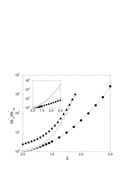
Figure 7: Mass anisotropy of the three-dimensional model (36). Circles: $\hbar\omega=1.0\,t_{x}$, $t_{z}=0.25\,t_{x}$; squares: $\hbar\omega=0.5\,t_{x}$, $t_{z}=0.25\,t_{x}$; triangles: $\hbar\omega=0.5\,t_{x}$, $t_{z}=0.1\,t_{x}$. Inset: masses $m^{\ast}_{xy}$ (filled circles) and $m^{\ast}_{z}$ for $\hbar\omega=1.0\,t_{x}$, $t_{z}=0.25\,t_{x}$. From anisotropy .

In relation to the effect described, it is interesting to note a well-documented discrepancy between the theoretical and experimental anisotropy of the cuprates Cooper1994 . According to band structure calculations, the anisotropy of resistivity of LSCO and YBCO compounds should be about $10-30$ Allen1987 ; Pickett1989 . At the same time, the experimental anisotropy of resistivity is between $10^{2}$ and $10^{3}$ depending on the level of doping. The anisotropy of bismuthates is even higher, $(5-80)\cdot 10^{4}$ Cooper1994 , which is difficult to explain with the conventional Bloch-Boltzmann theory. According to the present results, anisotropic interaction with $z$-polarized phonons is a sufficient condition for a very large $z$ effective mass. Of course, the anisotropy of mass and resistivity are two different things, but it would be fair to assume that the former is at least partially responsible for the latter (see, e.g., Cooper1994 page 85). This idea still awaits proper development. Alternative explanations of the anomalous $z$-transport exist as well AKM1996 .

4.3 Spectrum flattening and polaron density of states

A great power of the PIQMC method is the ability to calculate an entire polaron spectrum in any dimensionality in a single run, as was explained in Section 3.3. This opens up an exciting possibility to calculate the polaron density of states (DOS) $\rho(E)=N^{-1}\sum_{\bf K}\delta(E-E_{\bf K}+E_{0})$ by discretizing the energy interval and histogramming $E_{\bf K}$ values at the end of simulations. The polaron spectrum in the adiabatic limit ($t\gg\hbar\omega$) possesses an interesting property of flattening at large lattice momenta, which has been well documented in the literature Wellein1996 ; Wellein1997 ; Romero1998 ; Stephan1996 . In the weak-coupling limit, the flattening can be readily understood as hybridization between the bare electron spectrum and a momentum-independent phonon mode. The resulting polaron dispersion is cosine-like at small ${\bf K}$ and flat at large ${\bf K}$. As larger couplings this picture becomes less and less intuitive but the flattening remains as a matter of fact Levinson1973 . It is noteworthy that in large spatial dimensions the phase space is dominated by states with large momenta. If all those states have close energies, they should form a peak in the DOS close to the top of the polaron band. Exact PIQMC calculations have confirmed that this is indeed the case Kornilovitch1999 . The evolution of the DOS of the isotropic Holstein model with phonon frequency $\omega$ in two and three dimensions is shown in Fig. 8(a) and (b). In all the cases presented the polaron is fully developed, with the bandwidth much smaller than $\omega$.

At small $\omega$, DOS develops a massive peak at the top of the band. The peak is more pronounced in $d=3$ than in $d=2$. The van Hove singularities are absorbed in the peak and as such cannot be seen. With increasing $\omega$, the polaron spectrum approached the cosine-like shape in full accordance with the Lang-Firsov non-adiabatic formula. The respective DOS gradually assume the familiar shapes of tight-binding zones with renormalized hopping integrals. The van Hove singularities are clearly visible. These results have an interesting corollary for the Holstein model. At small-to-moderate $\omega$ in two and three dimensions, the bottom half of the polaron band contains a tiny minority of the total number of states (measured in low percentage points). In most real systems those states will be localized and hence irrelevant. All the system’s responses will be dominated by the states in the peak. The physical properties of these physically relevant states are going to be quite different from those of the ground state that are usually analyzed theoretically.

Figure 8: (a) and (b) The evolution of the density of states of the Holstein polaron with phonon frequency $\omega$ in $d=2$ and $3$, respectively. Each graph was obtained by calculating the polaron spectrum at 100,000 ${\bf K}$ points randomly distributed in the Brillouin zone, and histogramming the results between 50 energy bins. Each spectrum point was calculated by averaging 250,000 values of $\cos{{\bf K}\Delta{\bf r}}$ taken every 10th path update. Every 5000 measurements the path was reset and then equilibrated for 1000 updates. (c) The same for the small Fröhlich polaron in $d=2$.

It is interesting to look at the DOS of the long-range model (36). The two dimensional DOS is shown in Fig. 8(c). It is much closer to the tight-binding shape than the Holstein DOS at the same parameters. The polaron spectrum and density of states is another manifestation of the extremity of the Holstein model. Long-range e-ph interactions remove those peculiarities and make the polaron bands more “normal”.

Some densities of states of the Holstein model with anisotropic hopping were presented in Kornilovitch1999 .

4.4 Isotope exponents

Isotope substitution is a powerful tool in determining if a particular phenomenon or feature is of phonon origin. Some polaron properties, such as mass, are sharp functions of the lattice parameters, therefore isotope effects in (bi)polarons are strongly enhanced. In particular, anything that depends on the (bi)polaron mass should exhibit a large isotope exponent Alexandrov1992 . A large isotope effect was observed, for example, on the magnetic penetration depth in cuprates Zhao1997 ; Khasanov2004 ; Zhao2006 , which was interpreted as evidence for bipolaronic carriers in the superconducting state.

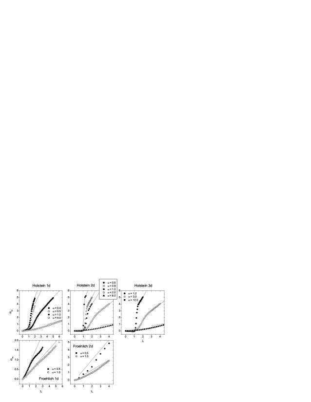
Figure 9: Mass isotope exponents of the small Holstein and small Fröhlich polarons in different dimensions and for different phonon frequencies. The thin solid lines indicate the strong-coupling limit $\alpha=\frac{\gamma}{2}\frac{\lambda zt}{\hbar\omega}$. Note that $\alpha$ of the Holstein polaron in $d=2$ and $3$ is negative at small $\omega$.

As was explained in Section 3.3, the PIQMC method enables approximation-free calculation of the isotope exponent on the (bi)polaron effective mass for a large class of e-ph models. A good feel for $\alpha$ in the strong-coupling limit can be obtained from the anti-adiabatic expression for the polaron mass, $m^{\ast}=m_{0}\,e^{\gamma(E_{p}/\hbar\omega)}$. Since the polaron shift $E_{p}$ is ion-mass-independent, $\alpha=\frac{\gamma}{2}\frac{E_{p}}{\hbar\omega}$. Thus $\alpha$ is proportional to the coupling constant $\lambda$. In the weak coupling regime, $\alpha$ can be computed perturbatively. For example, for the one-dimensional Holstein model, the second order yields

$$\alpha^{(2)}_{\rm 1d\>Holstein}=\lambda\frac{\bar{\omega}^{2}(\bar{\omega}^{2}+2\bar{\omega}+4)}{(\bar{\omega}^{2}+4\bar{\omega})^{\frac{5}{2}}}\>,$$ (39)

where $\bar{\omega}=\hbar\omega/t$. (The second-order coefficients of other polaron properties of the one-dimensional Holstein model can be found, e.g., in Spenser2005 . The second order coefficients for higher-dimensional lattices were given in Hague2005 .) The isotope exponent is again proportional to $\lambda$ but with a different coefficient. The two linear dependencies should be smoothly connected over the polaron crossover.

The mass isotope exponents for the small Holstein polaron are shown in the top row of Fig. 9. Before the polaron transition $\alpha$ is small reflecting the non-polaronic character of the carrier. Note that in $d=2$ and $3$, $\alpha$ is negative at small frequencies Hague2005 . After the polaron crossover, which always begins at $\lambda\sim 1$ but ends at $\lambda$ that increases with $\omega$, the isotope exponent quickly reaches the strong-coupling asymptotic behaviour with $\gamma=1$. Notice that the beginning and the end of the transition are clearly identifiable on the plots. Thus the mass isotope exponent can be useful in analyzing the Holstein polaron transition.

The case of the small Fröhlich polaron is somewhat different, see the bottom row of Fig. 9. At small coupling, the exponent grows linearly with a $\gamma$ close to the strong coupling limit, but then deviates to smaller values. The exponent returns back to the strong-coupling limit at much larger $\lambda$, whose value decreases with increasing $\omega$. This final approach happens when the entire path is mostly confined to one lattice site, and only rarely deviates to the first nearest neighbour. This interesting behaviour is not yet fully understood.

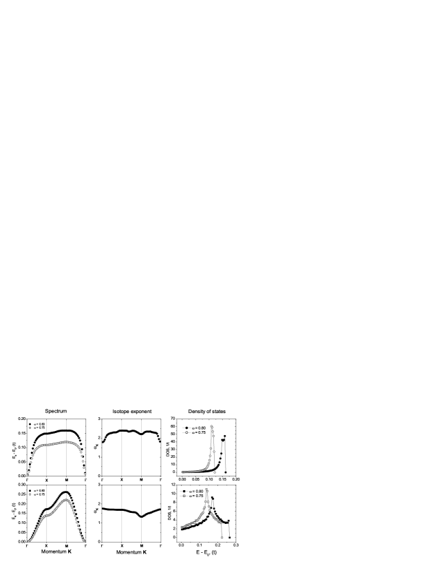
Figure 10: Isotope effect on polaron spectrum and density of states. Top row: the $2d$ Holstein polaron at $\lambda=1.2$. Left: polaron spectrum at $\bar{\omega}=0.80$ and $0.75$. Middle: the isotope exponent for each ${\bf K}$-point. Right: the density of states for the two frequencies. Bottom row: the same for the small $2d$ Fröhlich polaron at $\lambda=2.4$.

As was shown in the previous section, in the adiabatic regime the properties of the polaron mass do not fully represent those of the vast majority of polaron states. Additional insight can be gained from an isotope effect on the polaron bandwidth or even on individual spectrum points isotope . The isotope effect on polaron spectrum and density of states in $d=2$ is illustrated in Fig 10. The ratio of the two phonon frequencies, $\hbar\omega=0.80\,t$ and $0.75\,t$, has been chosen to roughly correspond to the substitution of ¹⁶O for ¹⁸O in complex oxides. One can see that the polaron band shrinks significantly, by 20-30%, for both polaron types. The middle panels show the isotope exponents on spectrum points calculated as

$$\alpha_{\bf K}=\frac{1}{2}\frac{\langle\omega\rangle}{\langle E_{\bf K}\rangle}\frac{\Delta E_{\bf K}}{\Delta\omega}\>,$$ (40)

where the angular brackets denote the mean value of either the two frequencies or of the two energy values. An interesting observation is that $\alpha_{\bf K}$ of the Fröhlich polaron is roughly independent of ${\bf K}$ ($\pm 10\%$). In the Holstein case $\alpha_{\bf K}$ dips in the vicinity of the ${\rm\Gamma}$ point. (Small fluctuations at intermediate momenta are due to statistical errors in averaging $\langle\cos{\bf K}\Delta{\bf r}\rangle$.)

4.5 Jahn-Teller polaron

Density-displacement is only one possible type of e-ph interaction. Examples of other types are the deformation potential and Su-Schrieffer-Heeger (SSH) interaction. In the former, the electron density interacts with a gradient of lattice displacement whereas in the SSH case the lattice deformation is coupled to electron’s kinetic energy. The Jahn-Teller (JT) interaction is one of the most complex types because it usually involves a multidimensional electron basis and a multidimensional representation of the deformation group. The JT interaction is active in some molecules and crystals of high point symmetry. The JT effect was also a guiding principle in the search for high-temperature superconductivity Bednorz1988 . More recently, a JT theory of the cuprates was developed in Mihailovic2001 ; Kabanov2002 ; Mertelj2005 . There exist different flavors of the JT interaction. The simplest one is the $E\otimes\,e$ interaction Kanamori1960 that describes a short-range coupling between twice-degenerate $e_{g}$ electronic levels $(c_{1},c_{2})$ and a local double-degenerate vibron mode $(\zeta,\eta)$. The Hamiltonian reads

$$H_{\rm JT}= - t\sum_{\langle{\bf nn^{\prime}}\rangle}\left(c^{\dagger}_{{\bf n^{\prime}}1}c_{{\bf n}1}+c^{\dagger}_{{\bf n^{\prime}}2}c_{{\bf n}2}\right)$$ (41)

$$- \kappa\sum_{\bf n}\left[\left(c^{\dagger}_{{\bf n}1}c_{{\bf n}2}+c^{\dagger}_{{\bf n}2}c_{{\bf n}1}\right)\eta_{\bf n}+\left(c^{\dagger}_{{\bf n}1}c_{{\bf n}1}-c^{\dagger}_{{\bf n}2}c_{{\bf n}2}\right)\zeta_{\bf n}\right]$$

$$+ \sum_{\bf n}\left[-\frac{\hbar^{2}}{2M}\left(\frac{\partial^{2}}{\partial\zeta^{2}_{\bf n}}+\frac{\partial^{2}}{\partial\eta^{2}_{\bf n}}\right)+\frac{M\omega^{2}}{2}\left(\zeta^{2}_{\bf n}+\eta^{2}_{\bf n}\right)\right]\>.$$

The symmetry of the interaction ensures the same coupling parameter $\kappa$ for the two phonons. The kinetic energy is chosen to connect like electron orbitals of the nearest neighbours. This choice is somewhat arbitrary (makes it more “Holstein-like”) and not dictated by symmetry. Because the ionic coordinates of different cells are not coupled, the model describes a collection of separate clusters that are linked only by electron hopping. To relate the Hamiltonian to more realistic situations, phonon dispersion must be added Mihailovic2001 ; Allen1999 .

An important property of the $E\otimes\,e$ interaction is the absence of an exact analytical solution in the atomic limit $t=0$. In the density-displacement case the dynamics of each $\zeta$ is described by a one-dimensional differential equation under a constant force. That has a shifted oscillator solution, which serves as a convenient starting point for various strong-coupling expansions. Here, in contrast, the atomic limit is described by two coupled partial differential equations for the electron doublet $\psi_{1,2}(\zeta,\eta)$. Although it is possible to separate variables and reduce the system to two ordinary second-order equations, they seem to be too complex to admit an analytical solution. At large couplings, however, the elastic energy assumes the Mexican hat shape and the phonon dynamics separates into radial oscillatory motion and azimythal rotary motion. This results in an additional pre-exponential factor $\propto\kappa$ in the ion overlap integral, leading to the effective mass $m^{\ast}_{\rm JT}=m_{0}\sqrt{\frac{2}{\pi g}}\,e^{g^{2}}$, where $g^{2}=\frac{\kappa^{2}}{2M\hbar\omega^{3}}$ Takada2000 .

A path integral approach to Hamiltonian (41) was developed in Kornilovitch2000 . Because there are two electron orbitals, the electron path must be assigned an additional orbital index (or colour) $a=1,2$. Colour 1 (or 2) of a given path segment means that it resides in the first (second) atomic orbital of the electron doublet. The short-term density matrix is

$$\rho(\Delta\tau) = \langle{\bf r^{\prime}}a^{\prime};\{\zeta^{\prime}_{\bf n}\}\{\eta^{\prime}_{\bf n}\}|e^{-\Delta\tau H}|{\bf r}a;\{\zeta_{\bf n}\}\{\eta_{\bf n}\}\rangle$$ (42)

$$= \left[\delta_{\bf rr^{\prime}}\delta_{aa^{\prime}}+(\kappa\Delta\tau)\delta_{\bf rr^{\prime}}\delta_{a{\bar{a}}^{\prime}}\eta_{\bf n}+(t\Delta\tau)\delta_{aa^{\prime}}\sum_{\bf l}\delta_{{\bf r^{\prime}},{\bf r}+{\bf l}}\right]e^{A_{\rm ph}(\Delta\tau)},$$

$$A_{\rm ph}(\Delta\tau)=(\kappa\Delta\tau)(\delta_{a1}-\delta_{a2})\zeta_{\bf n}$$

$$-\sum_{\bf n}\left\{\frac{M}{2\hbar^{2}(\Delta\tau)}[(\zeta_{\bf n}-\zeta^{\prime}_{\bf n})^{2}+(\eta_{\bf n}-\eta^{\prime}_{\bf n})^{2}]+(\Delta\tau)\frac{M\omega^{2}}{2}(\zeta^{2}_{\bf n}+\eta^{2}_{\bf n})\right\}.$$ (43)

Here ${\bar{a}}=1(2)$ when $a=2(1)$, that is ${\bar{a}}$ is “not” $a$. This expression reveals a difference between the two phonons. Phonon $\zeta$ is coupled to electron density, like in the Holstein case. The difference from the Holstein is that the direction of the force changes to the opposite when the electron changes orbitals. In contrast, phonon $\eta$ is coupled to orbital changes themselves: the more often the electron changes orbitals, the more “active” is $\eta$. (Discrete orbital changes are analogous to electron hops between discrete lattice sites, and as such are associated with “kinetic orbital energy”. Phonon coupling to orbital changes is analogous to phonon coupling to electron hopping in the Su-Schrieffer-Heeger interaction Su1979 .) Multiplication of a large number of the short-time propagators generates multiple terms, each of which contains a finite number of lattice hops and orbital changes. On top of that, the exponents combine in a total phonon action $A_{\rm ph}(\beta)$ that comprises the free $\eta$ action $A_{\eta 0}$ and the action of $\zeta$ phonons under an external force [$A_{\zeta}$ is similar to (21)]. The next step is integration over the paths $\eta(\tau)$ and $\zeta(\tau)$. Integration over $\zeta(\tau)$ is standard and performed as described as for the density-displacement interaction. The result is a factor $e^{A_{\zeta}}$ in the path’s statistical weight, where

$$A_{\zeta}[{\bf r}(\tau),a(\tau)]=\kappa^{2}\int^{\beta}_{0}\!\!\int^{\beta}_{0}{\rm d}\tau{\rm d}\tau^{\prime}G(\tau-\tau^{\prime})\left[\delta_{a(\tau),a(\tau^{\prime})}-\delta_{a(\tau),{\bar{a}}(\tau^{\prime})}\right]\>,$$ (44)

$$G(\tau-\tau^{\prime})=\frac{\hbar}{2M\omega}\left[e^{-\hbar\omega|\tau-\tau^{\prime}|}\delta_{{\bf r}(\tau),{\bf r}(\tau^{\prime})}+e^{-\hbar\omega(\beta-|\tau-\tau^{\prime}|)}\delta_{{\bf r}(\tau),{\bf r}(\tau^{\prime})+{\rm sgn}(\tau-\tau^{\prime})\Delta{\bf r}}\right]\!.$$ (45)

The last expression is valid under the condition $e^{\beta\hbar\omega}\gg 1$. As expected, action $A_{\zeta}$ is an explicit functional of the spatial path ${\bf r}(\tau)$ and of the orbital path $a(\tau)$. Note that the $\zeta$ phonon favours like orbitals and disfavours orbital changes. Integration over $\eta(\tau)$ is trickier for it contains $\eta$ as pre-exponential factors. A typical term with $N_{s}$ orbital changes has the following form:

$$(\kappa\Delta\tau)^{n}\eta_{{\bf r}(\tau_{1})}(\tau_{1})\eta_{{\bf r}(\tau_{2})}(\tau_{2})\ldots\eta_{{\bf r}(\tau_{N_{s}})}(\tau_{N_{s}})\,e^{A_{\eta 0}[\eta_{\bf n}(\tau)]}\>.$$ (46)

Here, $\tau_{s}$ is the time of $s$th orbital change ($s=1,\ldots,N_{s}$), ${\bf r}(\tau_{s})$ is the electron position at this time, and $\eta_{{\bf r}(\tau_{s})}(\tau_{s})$ is the $\eta$-displacement at this site at this time. For odd $N_{s}$, path integration over $\eta_{\bf n}(\tau)$ produces zero by parity. For even $m$, the integration can be performed by introducing fictitious sources, calculating the generating functional and differentiating it $m$ times. The result is a sum of all possible pairings of $\tau_{s}$. Within each term, each pair contributes the factor $\kappa^{2}G(\tau_{s}-\tau_{s^{\prime}})$, with $G$ given by (45). Since $G$ is positive, the statistical weight increases with the number of orbital flips. Thus, the $\eta$-phonon favours orbital flips, in complete contrast with the $\zeta$-phonon. Since both phonons are governed by the same Green’s function (which should be no surprise since the two phonons are related by symmetry) one should expect a dynamical equilibrium between the two phonons and some finite mean value of orbital flips for given coupling. The shift partition function is

$$Z_{\Delta{\bf r}}=Z_{\rm ph}\sum^{\infty}_{N_{k}=0,1,\ldots}\sum^{\infty}_{N_{s}=0,2,\ldots}\int^{\beta}_{0}\cdots\int^{\beta}_{0}({\rm d}\tau)^{N_{k}}({\rm d}\tau)^{N_{s}}W_{N_{k}N_{s}}\>,$$ (47)

$$W_{N_{k}N_{s}}=t^{N_{k}}\kappa^{N_{s}}\left[\prod_{{\rm(\>pairs\>of\>}\tau_{s}{\rm)}}G(\tau_{s}-\tau_{s^{\prime}})\right]\,e^{A_{\zeta}[{\bf r}(\tau),a(\tau)]}\>.$$ (48)

Compared to (27), the above expression involves additional multiple integration over the times of orbital flips. Each term is associated with a spatial-orbital path with $N_{k}$ kinks and $(N_{s}/2)$ $\eta$-phonon pairings, as shown in Fig. 11(a). A Markov process is organized by inserting/removing spatial kinks and by attaching/removing the pairing lines. The acceptance rules for the pairing lines can be derived by extending the method of Section 3.1 to two-time updates. For details see Kornilovitch2000 . The path shown in Fig. 11(a) can be considered a space-time diagram. In fact, the update process just described is a version of the Diagrammatic Monte Carlo method ProkofevDMC .

Figure 11: Extensions of the basic polaron PIQMC method. (a) In the Jahn-Teller polaron, the path carries an internal orbital index shown as black or white sections of the path. The $\eta$-phonon parings are represented by dashed lines. Each vertex changes the index. (b) In the bipolaron case, the system is represented by two imaginary-time paths. A direct configuration is shown on the left and an exchange one on the right. The interaction of segments marked A or B contribute to the energy of individual polarons. The segments that belong to different paths, such as those marked C, contribute to the interaction between the polarons.

After the update rules are established, the JT polaron properties can be calculated with no approximations. The mass, spectrum, and density of states are obtained as for the conventional lattice polarons. For the JT energy the thermodynamic estimator yields:

$$E_{0}=\left\langle-\frac{N_{k}}{\beta}-\frac{\partial A_{\zeta}}{\partial\beta}-\frac{N_{s}}{\beta}-\frac{\hbar\omega}{\beta}\sum_{G}\frac{1}{G(\tau_{s}-\tau_{s^{\prime}})}\frac{\partial G(\tau_{s}-\tau_{s^{\prime}})}{\partial(\hbar\omega)}\right\rangle_{\rm shift}.$$ (49)

The first two terms are familiar from the Holstein case. The first is the kinetic energy of the electron. The second is the potential energy of interaction with the $\zeta$ plus the (positive) elastic energy of $\zeta$. The other two terms are new. The third one represents the negative “orbital energy” caused by orbital flips. These processes excite phonons $\eta$, which results in the positive fourth term.

The number of excited phonons is an important characteristic because it provides an internal consistency check for the algorithm: one expects equal mean number of $\zeta$ and $\eta$ phonons. The phonon number estimator is derived as the derivative of the free energy with respect to $(\hbar\omega)$ under a fixed combination $\kappa^{2}/(M\omega)$. One obtains

$$N_{{\rm ph},\zeta}=-\frac{1}{\beta}\left\langle\left.\frac{\partial A_{\zeta}}{\partial(\hbar\omega)}\right|_{\frac{\kappa^{2}}{M\omega}}\right\rangle_{\rm shift},$$ (50)

$$N_{{\rm ph},\eta}=-\frac{1}{\beta}\left\langle\sum_{G}\frac{1}{G(\tau_{s}-\tau_{s^{\prime}})}\frac{\partial G(\tau_{s}-\tau_{s^{\prime}})}{\partial(\hbar\omega)}\right\rangle_{\rm shift}.$$ (51)

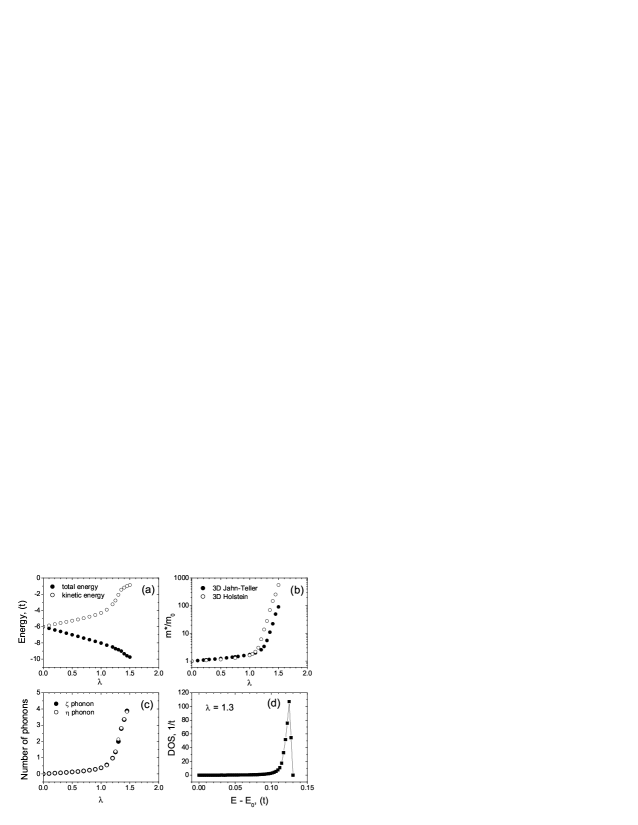
Figure 12: Physical properties of the $d=3$ Jahn-Teller polaron at $\hbar\omega=1.0\,t$ Kornilovitch2000 . (a) The total and kinetic energy. (b) The effective mass compared with the $d=3$ Holstein polaron at the same phonon frequency. (c) The number of excited phonons of both types. (d) The density of states of the JT polaron at $\lambda=1.3$.

Results of PIQMC calculations are shown in Fig. 12 Kornilovitch2000 . Most properties behave similarly to those of the $d=3$ Holstein polaron at the same phonon frequency, $\hbar\omega=1.0\,t$. For example, the kinetic energy, Fig. 12(a), sharply decreases by absolute value between $\lambda=1.2$ and $1.4$. The JT polaron mass is slightly larger at the small to intermediate coupling, but several times smaller at the strong coupling. This non-monotonic behaviour of the ratio of the JT and Holstein masses was later confirmed by accurate variational calculations ElShawish2003 , although in that work the JT polaron (and bipolaron) was investigated in one spatial dimension. The relative lightness of the JT polaron is consistent with Takada’s result mentioned above Takada2000 . The number of excited phonons of both types is shown in Fig. 12(c). As expected, numerical values coincide within the statistical error, which validates the numerical algorithm. Interestingly, the shape of the phonon curves is similar to that of the logarithm of the effective mass. This suggests an intimate relationship between the two quantities, again similarly to the Holstein case. Finally, the density of JT polaron states features the same peak at the top of the band, caused by the spectrum flattening at large polaron momenta.

In summary, the locality of the JT interaction and the independence of vibrating clusters result in the same extremity of polaron properties as in the $3d$ Holstein model. One should expect that either a long-range JT or phonon dispersion will soften the sharp polaron features and make them more “normal”. This is an interesting research opportunity for the PIQMC method.

5 Prospects

In this Chapter, a theoretical approach to lattice polarons based on the statistical path integral has been developed. A characteristic feature of the method is a tight integration of analytical and numerical elements within one technique. The numerical part of the algorithm is greatly aided by the preliminary analytical steps: path integration over the ionic coordinates and reduction of the double integral over imaginary time to a discrete sum over path segments. Thus, on the way from the Hamiltonian to observables, exact analytical transformations are carried as far as possible increasing the accuracy and speed of the simulations.

The PIQMC polaron method is still very much under development. Due to the space constraints, only key elements have been presented here and many technical details have been left out. This concluding section will be used to outline various extensions of the method. Some of them have already been done, others can be done but await proper implementation. Certain problems have not yet been solved even on the conceptual level, and those will be discussed too.

5.1 Bipolaron

The possibility of two polarons forming bound pairs, or bipolarons, opens a whole new dimension in polaron physics Alexandrov1995 ; Devreese1996 . The two major competing factors are the phonon-mediated attraction between the polarons that favours paring and direct Coulombic repulsion that prevents pairing. Kinetic energy, exchange effects and short-range lattice effects play important supporting roles that can tip the balance toward or against paring. All of this may lead to a rich and complex phase diagram. The bipolaron concept has been well-developed in the literature. The large continuous-space (Fröhlich) bipolaron in ionic media was considered in Verbist1990 ; Hiramoto1985 ; Emin1992 , and the small, localized, lattice bipolaron in Anderson1975 . Since the bipolarons are charged bosons at low density $n$, they can superconduct below the Bose-Einstein condensation temperature

$$T_{\rm BE}=3.31\frac{\hbar^{2}}{k_{B}}\frac{n^{2/3}}{m^{\ast\ast}}\>.$$ (52)

The concept of mobile lattice bipolarons and bipolaronic superconductivity was put forward by Alexandrov and Ranninger in 1981 Alv81 and since then thoroughly developed by Alexandrov and co-workers Alexandrov1996 ; Kornilovitch2002 ; Alexandrov1992 ; AKM1996 ; Alv93 ; AlvM94 ; Alv03 ; Alexandrov2006 . Note that $T_{\rm BE}$ is inversely proportional to the bipolaron mass. This suggests the following recipe to increase the critical temperature according to the bipolaronic mechanism: reduce the effective mass while keeping the bipolarons non-overlapping. (Clearly, simply reducing the mass will increase the bipolaron radius and reduce the overlap density. There is a trade-off between the $n^{2/3}$ and $(m^{\ast\ast})^{-1}$ factors in (52), which creates a challenging optimization problem.)

As with polarons, the first application of path integrals to the bipolaron was to the continuum-space Fröhlich bipolaron Verbist1990 ; Hiramoto1985 . Until very recently, the only application of path integrals to the lattice bipolaron was the work by de Raedt and Lagendijk DeRaedtBipolaron on the discrete-time version of their path-integral QMC method. The authors limited the consideration to the extreme adiabatic limit and computed the phase diagram of the Holstein bipolaron with an additional Hubbard repulsion. A continuous-time version of PIQMC was developed very recently and the first results presented in Hague2006 .

The lattice bipolaron, mostly with Holstein interaction, has been studied by a variety of other numerical methods: exact diagonalization Wellein1996 ; Weisse2000 , variational Bonca2000 ; Bonca2001 ; ElShawish2003 , density matrix renormalization group Zhang1999 , diagrammatic quantum Monte Carlo Macridin2004 , and Lang-Firsov quantum Monte Carlo Hohenadler2005 ; Hohenadler2005b .

Conceptually, generalizing the PIQMC method to the bipolaron is straightforward. There are two paths that visualize the imaginary-time evolution of the two fermions. To enable calculation of the effective mass, open boundary conditions in imaginary time must be used: the top ends of the paths must be the same as the bottom ones up to an arbitrary lattice translation $\Delta{\bf r}$. Singlet and triplet states can be separated by allowing the paths to exchange, see Fig. 11(b). Then the bipolaron spectrum, mass, and singlet-triplet splitting is calculated as explained in Section 2. Phonon integration is performed as before with the same resulting action, (22)-(26). The difference is the force that is acting on the oscillator ${\bf m}$ at time $\tau$. In a bipolaron system it receives contribution from both electrons, $f_{\bf m}(\tau)=f_{\bf m}[{\bf r}_{1}(\tau)]+f_{\bf m}[{\bf r}_{2}(\tau)]$. Since the action is quadratic in $f$, it becomes a sum of three terms that contain the products $f[{\bf r}_{1}(\tau)]f[{\bf r}_{1}(\tau^{\prime})]$, $f[{\bf r}_{2}(\tau)]f[{\bf r}_{2}(\tau^{\prime})]$, and $f[{\bf r}_{1}(\tau)]f[{\bf r}_{2}(\tau^{\prime})]$, respectively. The first two terms describe the retarded self-interaction of the two paths and are responsible for polaron formation. The third cross-term describes the interaction between the paths. It is responsible for the interaction between the polarons and for bipolaron formation. This is illustrated in Fig. 11(b). The estimators for various observables and specific expressions for the segment-to-segment contributions are derived analogously to the polaron case. Technical details of the derivation have not yet been published, and will be published elsewhere.

One interesting effect that has already been considered by the PIQMC method is the “crab-like” bipolaron that can exist on certain lattices Hague2006 . Usually, the bipolaron is much heavier that the constituent polarons, its mass scaling as the second power of the polaron mass in the non-adiabatic regime and as the fourth power in the adiabatic limit Alexandrov1986 . (Path integrals provide a useful visualization of this effect, see Fig. 11(b). At a small phonon frequency, the two paths interact over their entire length. Therefore they are much more difficult to separate, which results in slower imaginary-time diffusion, and hence a heavier particle.) However, on the triangular, face-centered cubic and some other lattices the intersite bipolaron can move without breaking. This results in an effective mass that scales only linearly with the polaron mass. This effect was predicted some time ago by Alexandrov Alexandrov1996 , and recently confirmed by exact PIQMC simulations in Hague2006 .

5.2 Further extentions

Recall that the basic Hamiltonian (12) contains the simplest possible form of the electron kinetic energy and the simplest possible model of the crystal lattice. It will now be explained how to relax these restrictions. First of all, it is straightforward to add electron hopping beyond the nearest neighbours. Because the path is defined in real space, this only requires the introduction of additional kink types that move the path in the respective directions. The values of the distant hopping integrals can be absolutely independent of the nearest-neighbour values as long as they are negative. The methods of Section 3.1 is readily generalized to paths containing kinks of different magnitude. The statistical weight (15) is now a product of factors $(t_{i}\Delta\tau)$ along the path. The stochastic acceptance rules now contain the factor $(t_{i}\beta)$ where $t_{i}$ is the hopping amplitude of the proposed kink. It is interesting though that contribution to the kinetic energy is the same (equal to $\beta^{-1}$) for all kinks independently of the $t_{i}$ value. It is the mean number of kinks that is affected by $t_{i}$, leading to different partial kinetic energies along different lattice directions. In exactly the same manner one can study models with anisotropic (but nearest-neighbour) electron hopping. This was done in Kornilovitch1999 ; anisotropy , cf. Section 4.2. There remains one important restriction on the values of the hopping amplitudes: they all must be negative to ensure the positivity of the path’s statistical weight. If even a single $t_{i}$ is positive, some paths will continue being positive but some will have negative weights. That will introduce a sign-problem, which will eventually render the simulation numerically unstable. Another extension related to the kinetic energy is lattices of different symmetries. Again, all that is changed is the table of kink types that specifies which two spatial points (lattice sites) each particular kinks connects. In this way, PIQMC has been applied to the triangular, face-centred-cubic, and hexagonal Bravais lattices in Hague2005 .

It should be mentioned that PIQMC can also simulate the (bi)polaron in dimensionalities larger than 3, see Fig. 3. (The $d=4$ Holstein polaron was previously investigated in Ku2002 .) Although such calculations have little practical value, they can still be useful in assessing the accuracy of approximate methods that rely on the number of spatial dimensions being large. (An example of such a method would be the Dynamical Mean Field Theory Capone2003 .)

Consider now the phonon subsystem. It is well-known that a bosonic path integral can be calculated analytically for any quadratic action. This means that the ionic coordinates can be eliminated even when they are coupled, that is in the case of dispersive phonons. Moreover, integration can be done for any number of degrees of freedom per unit cell. De Raedt and Lagendijk studied a one-dimensional Holstein polaron with phonon dispersion as early as in 1984 DeRaedt1984 . They found that the critical coupling of polaron formation decreases as the phonon mode becomes soft. To our knowledge, this remains the only exact analysis of a model with dispersive phonons to-date. A general phonon integration for the purposes of PIQMC method was performed in multiphonon . Conceptually, the result is similar to (22)-(27). The action is a sum of a periodic contribution and a correction due to the shifted boundary conditions. The action is a double integral over the imaginary time. However, there is an additional sum over the phonon momentum and branches. In addition, the action involves the eigenvalues and eigenvectors of the dynamical matrix. Thus, the polaron action comprises full information about the phonon spectrum and polarizations.

An important advantage of the PIQMC method is the ability to study temperature effects. At a finite temperature $T$, the projected partition function $Z_{\bf K}$ receives contributions from high-energy states with momentum ${\bf K}$. It is therefore not meaningful to calculate the polaron mass and spectrum. Instead, the conventional periodic boundary conditions in imaginary time must be used, which makes all states contribute to the full thermodynamic partition function $Z$. The parameter $\Delta{\bf r}$ is set to zero. The remaining periodic action (23) is valid at any temperature, large or small. This enables approximation free calculation of thermodynamic properties of the polaron: the internal energy, specific heat, number of excited phonons, and static e-ph correlation functions.

The grand challenge for PIQMC, as for almost any Quantum Monte Carlo method is efficient simulation of many-body systems. If the number of particles is three or more, the fermionic sign-problem is in general unavoidable. It is possible that the sign-problem in many-fermion e-ph models will be less severe that in the case of repulsive electron-electron models. Consider the limit of low electron density and strong e-ph interaction. The polarons will be bound in bipolarons, and the paths will fluctuate in pairs. To account for statistics, the top path ends must be constantly permuted, with even/odd permutations contributing $+1/-1$ phase factor to the partition function. However, any odd permutation will have to separate a path pair. This will increase the energy of the configuration and such an update will likely be rejected. In contrast, some even permutations will exchange whole bipolarons, which will keep the paths together with no significant energy increase. Such updates will likely be accepted. As a result, there will be many more even than odd permutations, and the average sign will be well defined. The stronger the coupling the more pronounced this effect will be, and the more the system will approach a purely bosonic limit (which is sign-problem-free).

The temperature-control capability offers another unique opportunity: calculation of the Meissner fraction and superconducting critical temperature. The method was devised by Scalapino et al Scalapino1993 and is based on the sum rule for the off-diagonal current-current correlation function. By comparing its static limit with the kinetic energy, one could determine a temperature at which the two quantities start to differ. This signifies the appearance of a Meissner fraction and determines the $T_{c}$.

Finally, we comment on the calculation of dynamical (bi)polaron properties such as the spectral function or optical conductivity. This is a classic and difficult problem for most existing Monte Carlo methods. Derivation of real-time correlators from imaginary-time correlators amounts to solving an ill-posed inversion problem, which is usually regularized by methods such as maximum entropy Jarrell_1996 , Pade approximants, or stochastic optimization Mishchenko2000 . Any of this techniques can be used in conjunction with the PIQMC method.

5.3 Conclusions

In summary, path integrals have played and continue to play an important role in the development of polaron physics. The path-integral quantum Monte Carlo method has proven to be a powerful and versatile tool. It has some unique advantages, such as system-size independence, the ability to calculate the density of states, mass isotope exponents, and temperature effects. Compared to the exact diagonalization, density-matrix renormalization group, or variational methods, PIQMC has a larger statistical error, but provides unbiased estimates for the (bi)polaron properties. Several novel qualitative results have been obtained with the PIQMC method: small polaron mass in models with long-range electron-phonon interaction, enhancement of the anisotropy of the polaron spectrum, a peak in the polaron density of states in the adiabatic limit, and the isotope effect on the polaron spectrum. These and some other effects have been discussed in this Chapter in detail.

References

- (1) P.A.M. Dirac: Physikalische Zeitschrift der Sowjetunion 3, 64 (1933)
- (2) R.P. Feynman: Rev. Mod. Phys. 20, 367 (1948)
- (3) M. Kac: Trans. Am. Math. Soc. 65, 1 (1949)
- (4) R.P. Feynman: Phys. Rev. 97, 660 (1955)
- (5) H. Fröhlich, H. Pelzer, S. Zienau: Philos. Mag. 41, 221 (1950); H. Fröhlich: Advan. Phys. 3, 325 (1954); H. Fröhlich: Introduction to the theory of the polaron. In: Polarons and Excitons, ed by C.G. Kuper, G.D. Whitfield (Plenum Press, New York 1963) pp 1–32, and references therein
- (6) J.T. Devreese, R. Evrard: Phys. Lett. 23, 196 (1966)
- (7) N.V. Prokof’ev, B.V. Svistunov: Phys. Rev. Lett. 81, 2514 (1998)
- (8) A.S. Mishchenko, N.V. Prokof’ev, A. Sakamoto, B.V. Svistunov: Phys. Rev. B 62, 6317 (2000)
- (9) Y. Ōsaka: Prog. Theor. Phys. 22, 437 (1959)
- (10) R. Abe, K. Okamoto: J. Phys. Soc. Jpn. 31, 1337 (1971); 33, 343 (1972)
- (11) M. Saitoh: J. Phys. Soc. Jpn. 49, 878 (1980)
- (12) V.K. Fedyanin, C. Rodriguez: Physica A 112, 615 (1982)
- (13) G. De Filippis, V. Cataudella, V. Marigliano Ramaglia, C.A. Perroni and D. Bercioux: Eur. Phys. J. B 36, 65 (2003)
- (14) R.P. Feynman, R.W. Hellwarth, C.K. Iddings, P.M. Platzman: Phys. Rev. 127, 1004 (1962)
- (15) K.K. Thornber, R.P. Feynman: Phys. Rev. B 1, 4099 (1970)
- (16) F.M. Peeters, J.T. Devreese: Theory of polaron mobility. In: Solid State Physics, vol 38, ed by F. Seitz, D. Turnbull (Academic Press, New York 1984) pp 81–133
- (17) J.T. Devreese: Optical properties of few and many Fröhlich polarons from 3D to 0D. In: this volume; and references therein
- (18) F.M. Peeters, J.T. Devreese: Phys. Rev. B 25, 7281 (1982)
- (19) J.T. Devreese, F. Brosens: Phys. Rev. B 45, 6459 (1992)
- (20) G. Verbist, F.M. Peeters, J.T. Devreese: Solid State Commun. 76, 1005 (1990); Phys. Rev. B 43, 2712 (1991)
- (21) C. Alexandrou, W. Fleischer, R. Rosenfelder: Phys. Rev. Lett. 65, 2615 (1990)
- (22) C. Alexandrou, R. Rosenfelder: Phys. Rep. 215, 1 (1992)
- (23) F. Brosens, S.N. Klimin, J.T. Devreese: Phys. Rev. B 71, 214301 (2005)
- (24) H. de Raedt, A. Lagendijk: Phys. Rev. Lett. 49, 1522 (1982); Phys. Rev. B 27, 6097 (1983)
- (25) H. de Raedt, A. Lagendijk: Phys. Rep. 127, 234 (1985)
- (26) N. Metropolis, A.W. Rosenbluth, M.N. Rosenbluth, A.H. Teller, E. Teller: J. Chem. Phys. 21, 1987 (1953)
- (27) H. de Raedt, A. Lagendijk: Phys. Rev. B 30, 1671 (1984)
- (28) H. de Raedt, A. Lagendijk: Z. Phys. B: Condens. Matter 65, 43 (1986)
- (29) P.E. Kornilovitch, E.R. Pike: Phys. Rev. B 55, 8634 (1997); 69, 059902 (2004)
- (30) P.E. Kornilovitch: Phys. Rev. B 60, 3237 (1999)
- (31) P.E. Kornilovitch: Phys. Rev. Lett. 81, 5382 (1998)
- (32) A.S. Alexandrov, P.E. Kornilovitch: Phys. Rev. Lett. 82, 807 (1999)
- (33) P.E. Kornilovitch: Phys. Rev. B 59, 13531 (1999)
- (34) P.E. Kornilovitch: Phys. Rev. Lett. 84, 1551 (2000)
- (35) P.E. Kornilovitch, A.S. Alexandrov: Phys. Rev. B 70, 224511 (2004)
- (36) P.E. Spencer, J.H. Samson, P.E. Kornilovitch, A.S. Alexandrov: Phys. Rev. B 71, 184310 (2005)
- (37) J.P. Hague, P.E. Kornilovitch, A.S. Alexandrov, J.H. Samson: Phys. Rev. B 73, 054303 (2006)
- (38) P.E. Kornilovitch: Phys. Rev. B 73, 094305 (2006)
- (39) J.P. Hague, P.E. Kornilovitch, J.H. Samson, A.S. Alexandrov: Phys. Rev. Lett. 98, 037002 (2007)
- (40) J.E. Hirsch, E. Fradkin: Phys. Rev. Lett. 49, 402 (1982); Phys. Rev. B 27, 4302 (1983)
- (41) J.E. Hirsch, E. Fradkin: Phys. Rev. B 27, 1680 (1983)
- (42) A.S. Mishchenko, N. Nagaosa, N.V. Prokof’ev, A. Sakamoto, B.V. Svistunov: Phys. Rev. Lett. 91, 236401 (2003)
- (43) A.S. Mishchenko, N. Nagaosa: Phys. Rev. Lett. 93, 036402 (2004)
- (44) A. Macridin, G.A. Sawatzky, M. Jarrell: Phys. Rev. B 69, 245111 (2004)
- (45) A.S. Mishchenko, N. Nagaosa: Spectroscopic properties of polarons in strongly correlated systems by exact diagrammatic Monte Carlo method. In: this volume
- (46) M. Hohenadler, H.G. Evertz, W. von der Linden: Phys. Rev. B 69, 024301 (2004)
- (47) M. Hohenadler, W. von der Linden: Phys. Rev. B 71, 184309 (2005)
- (48) M. Hohenadler, W. von der Linden: Lang-Firsov approaches to polaron physics: From variational methods to unbiased quantum Monte Carlo simulations. In: this volume
- (49) A.S. Alexandrov, V.V. Kabanov, D.K. Ray: Phys. Rev. B 49, 9915 (1994)
- (50) G. Wellein, H. Röder, H. Fehske: Phys. Rev. B 53, 9666 (1996)
- (51) G. Wellein, H. Fehske: Phys. Rev. B 56, 4513 (1997)
- (52) H. Fehske, J. Loos, G. Wellein: Phys. Rev. B 61, 8016 (2000)
- (53) F.X. Bronold, H. Fehske: Phys. Rev. B 66, 073102 (2002)
- (54) H. Fehske, S.A. Trugman: Numerical solution of the Holstein polaron problem. In: this volume
- (55) A.H. Romero, D.W. Brown, K. Lindenberg: J. Chem. Phys. 109, 6540 (1998); Phys. Rev. B 59, 13728 (1999)
- (56) J. Bonča, S.A. Trugman, I. Batistić: Phys. Rev. B 60, 1633 (1999)
- (57) J. Bonča, T. Katrašnik, S.A. Trugman: Phys. Rev. Lett. 84, 3153 (2000)
- (58) J. Bonča, S.A. Trugman: Phys. Rev. B 64, 094507 (2001)
- (59) Li-Chung Ku, S.A. Trugman, J. Bonča: Phys. Rev. B 65, 174306 (2002)
- (60) E. El Shawish, J. Bonča, Li-Chung Ku, S.A. Trugman: Phys. Rev. B 67, 014301 (2003)
- (61) V. Cataudella, G. De Filippis, G. Iadonisi: Phys. Rev. B 62, 1496 (2000)
- (62) C.A. Perroni, V. Cataudella, G. De Filippis: J. Phys.: Condensed Matter 16, 1593 (2004)
- (63) V. Cataudella, G. De Filippis, C.A. Perroni: Single polaron properties in different electron phonon models. In: this volume.
- (64) E. Jeckelmann, S.R. White: Phys. Rev. B 57, 6376 (1998)
- (65) E. Jeckelmann, C. Zhang, S.R. White: Phys. Rev. B 60, 7950 (1999)
- (66) C. Zhang, E. Jeckelmann, S.R. White: Phys. Rev. B 60, 14092 (1999)
- (67) T. Holstein: Ann. Phys. 8, 325 (1959); Ann. Phys. 8, 343 (1959)
- (68) G. Wellein, H. Fehske, A.P. Kampf: Phys. Rev. Lett. 81, 3956 (1998)
- (69) A. Weiße, H. Fehske: Phys. Rev. B 58, 13526 (1998)
- (70) A.S. Alexandrov: Phys. Rev. B 53, 2863 (1996); Phys. Rev. Lett. 82, 2620 (1999)
- (71) A.S. Alexandrov, P.E. Kornilovitch: J. Phys.: Condensed Matter 14, 5337 (2002)
- (72) P.E. Kornilovitch: Phys. Rev. B 71, 094301 (2005)
- (73) M. Boninsegni, D.M. Ceperley: Phys. Rev. Lett. 74, 2288 (1995)
- (74) K. Binder, ed: Monte Carlo Methods in Statistical Physics, Topics in Current Physics No. 7 (Springer, New York 1978)
- (75) K. Binder, ed: Applications of the Monte Carlo Method in Statistical Physics, Topics in Current Physics No. 36 (Springer, New York 1984)
- (76) K. Binder, ed: The Monte Carlo Method in Condensed Matter Physics, Topics in Applied Physics No. 71 (Springer, New York 1995)
- (77) D.M. Ceperley: Rev. Mod. Phys. 67, 279 (1995)
- (78) W.M.C. Foulkes, L. Mitas, R.J. Needs, G. Rajagopal: Rev. Mod. Phys. 73, 33 (2001)
- (79) M.C. Gordillo, D.M. Ceperley: Phys. Rev. B 58, 6447 (1998)
- (80) G.H. Bauer, D.M. Ceperley, N. Goldenfeld: Phys. Rev. B 61, 9055 (2000)
- (81) D.M. Ceperley, B. Bernu: Phys. Rev. Lett. 93, 155303 (2004)
- (82) B.K. Clark, D.M. Ceperley: Phys. Rev. Lett. 96, 105302 (2006)
- (83) N.V. Prokof’ev, B.V. Svistunov, I.S. Tupitsyn: Zh. Eksp. Teor. Fiz. 114, 570 (1998) [Sov. Phys. JETP 87, 310 (1998)]
- (84) R.P. Feynman: Statistical mechanics (Benjamin, Reading 1972) pp 78–84 (chapter 3)
- (85) P.E. Kornilovitch: Phys. Rev. B 71, 094301 (2005)
- (86) A.S. Alexandrov: Phys. Rev. B 46, 14932 (1992)
- (87) D.M. Eagles: Phys. Rev. 145, 645 (1966); Phys. Rev. 181, 1278 (1969)
- (88) T. Timusk et al. In: Anharmonic Properties of High- Cuprates, ed by D. Mihailović et al (World Scientific, Singapore, 1995) pp 171
- (89) S.V. Tjablikov: Zh. Eksp. Teor. Fiz. 23, 381 (1952)
- (90) I.G. Lang, Yu.A. Firsov: Zh. Eksp. Teor. Fiz. 43, 1843 (1962) [Sov. Phys. JETP 16, 1301 (1963)]
- (91) S.L. Cooper, K.E. Gray: Anisotropy and interlayer coupling in the high- cuprates. In: Physical Properties of High-Temperature Superconductors, vol IV, ed by D.M. Ginsberg (World Scientific, Singapore 1994) pp 61–188
- (92) P.B. Allen, W.E. Pickett, H. Krakauer: Phys. Rev. B 36, 3926 (1987)
- (93) W.E. Pickett: Rev. Mod. Phys. 61, 433 (1989)
- (94) A.S. Alexandrov, V.V. Kabanov, N.F. Mott: Phys. Rev. Lett. 77, 4796 (1996)
- (95) W. Stephan: Phys. Rev. B 54, 8981 (1996)
- (96) Y.B. Levinson, E.I. Rashba: Rep. Prog. Phys. 36, 1499 (1973)
- (97) G. Zhao, M.B. Hunt, H. Keller, K.A. Müller: Nature 385, 236 (1997)
- (98) R. Khasanov, D.G. Eshchenko, H. Luetkens, E. Morenzoni, T. Prokscha, A. Suter, N. Garifianov, M. Mali, J. Roos, K. Conder, H. Keller: Phys. Rev. Lett. 92, 057602 (2004)
- (99) Guo-meng Zhao: Polarons in colossal magnetoresistive and high-temperature superconducting materials. In: this volume
- (100) J.G. Bednorz, K.A. Müller: Rev. Mod. Phys. 60, 585 (1988)
- (101) D. Mihailovic, V.V. Kabanov: Phys. Rev. B 63, 054505 (2001)
- (102) V.V. Kabanov, D. Mihailovic: Phys. Rev. B 65, 212508 (2002)
- (103) T. Mertelj, V.V. Kabanov, D. Mihailovic: Phys. Rev. Lett. 94, 147003 (2005)
- (104) J. Kanamori: J. Appl. Phys. 31, S14 (1960)
- (105) P.B. Allen, V. Perebeinos: Phys. Rev. B 60, 10747 (1999)
- (106) Y. Takada: Phys. Rev. B 61, 8631 (2000)
- (107) W.P. Su, J.R. Schrieffer, A.J. Heeger: Phys. Rev. Lett. 42, 1698 (1979)
- (108) A.S. Alexandrov, N.F. Mott: Polarons and Bipolarons (World Scientific, Singapore 1995)
- (109) J.T. Devreese: Polarons. In: Encyclopedia of Applied Physics, vol 14 (VCH Publishers 1996) pp 383–413
- (110) H. Hiramoto, Y. Toyozawa: J. Phys. Soc. Japan 54, 245 (1985)
- (111) D. Emin, J. Ye, C.L. Beckel: Phys. Rev. B 46, 10710 (1992)
- (112) P.W. Anderson: Phys. Rev. Lett. 34 953 (1975)
- (113) A.S. Alexandrov, J. Ranninger: Phys. Rev. B 23, 1796 (1981); Phys. Rev. B 24, 1164 (1981)
- (114) A.S. Alexandrov: Phys. Rev. B 48, 10571 (1993)
- (115) A.S. Alexandrov, N.F. Mott: High-Temperature Superconductors and Other Superfluids (Taylor & Fransis Springer, London 1994)
- (116) A.S. Alexandrov: Theory of Superconductivity: From Weak to Strong Coupling (IoP Publishing, Bristol and Philadelphia, 2003)
- (117) A.S. Alexandrov: Superconducting polarons and bipolarons. In: this volume
- (118) A. Weiße, H. Fehske, G. Wellein, A.R. Bishop: Phys. Rev. B 62, 747 (2000)
- (119) M. Hohenadler, M. Aichhorn, W. von der Linden: Phys. Rev. B 71, 014302 (2005)
- (120) A.S. Alexandrov, V.V. Kabanov: Sov. Phys. Solid State 28, 631 (1986)
- (121) M. Capone, S. Ciuchi: Phys. Rev. Lett. 91, 186405 (2003)
- (122) D.J. Scalapino, S.R. White, S. Zhang: Phys. Rev. B 47, 7995 (1993)
- (123) M. Jarrell, J. Gubernatis: Phys. Rep. 269, 133 (1996)