Temperature-extended Jarzynski relation:
Application to the numerical calculation of the surface tension

Abstract

We consider a generalization of the Jarzynski relation to the case where the system interacts with a bath for which the temperature is not kept constant but can vary during the transformation. We suggest to use this relation as a replacement to the thermodynamic perturbation method or the Bennett method for the estimation of the order-order surface tension by Monte Carlo simulations. To demonstrate the feasibility of the method, we present some numerical data for the 3D Ising model.

1 Introduction

In the last decade, important progresses have been made in the context of far-from-equilibrium statistical physics with the derivation of the so-called fluctuation theorems. Among these theorems, the Jarzynski relation has certainly become the most famous one and is now widely applied both in experimental and numerical studies not only in physics but in chemistry or biophysics as well. Remarkably, this relation relates thermodynamic equilibrium quantities to out-of-equilibrium averages over all possible histories of the system when submitted to a well-defined protocol. The system is initially prepared at thermal equilibrium and then driven out-of-equilibrium by varying a control parameter $h$ from say $h_{1}$ to $h_{2}$. The work $W$ is recorded for each experiment. The Jarzynski relation states that

$$e^{-\beta\Delta F}=\langle e^{-\beta W}\rangle$$ (1)

where $\Delta F$ is the free-energy difference $\Delta F=F(h_{2})-F(h_{1})$ between the two equilibrium states at values $h_{1}$ and $h_{2}$ of the control parameter. In his first paper on the subject, Jarzynski gave a derivation of this relation in the case of a set of particles evolving according to the laws of Newtonian mechanics [1]. The derivation depends crucially on the assumption that the system is initially thermalized with a heat bath at temperature $T$ but then isolated from it while the work is exerted. No exchange of heat with the environment is possible. A change of the temperature of the bath has thus no consequence. In a second paper [2], Jarzynski showed that the relation (1) may be established in the case of a Markovian dynamics too. In this case, the interaction with the bath is encoded in the transition rates. The demonstration does not require anymore the insulation of the system from the bath while the work is exerted. Exchange of heat with the environment is properly taken into account during the whole process.

It is a simple exercise to generalize the Jarzynski relation to the case where the temperature of the heat bath changes with time. In the special case where no work is exerted on the system, one obtains (24):

$$e^{-\Delta(\beta F)}=\langle e^{-\int E(t)\dot{\beta}dt}\rangle$$ (2)

where $E(t)$ is the total energy of the system at time $t$. The derivation can be found in the appendix. As noted by Crooks in his dissertation [3] “it is possible to view this change as an additional perturbation that exerts a sort of entropic work on the system”. Like any other Jarzynski relation, Eq. (2) is also a special case of the annealed importance sampling method [4]. As far as we know, the case of a varying temperature has not attracted any attention. The aim of this paper is to show that a Jarzynski relation generalized to a temperature change may also have some interesting applications and deserves interest. As an example, we propose a new way to estimate by Monte Carlo simulations the order-order surface tension. This method is tested for the three-dimensional Ising model. The surface tension is related to the remaining free energy of a system containing two phases in coexistence separated by an interface when the contribution of these bulk phases has been removed. The Jarzynski relation offers the possibility to calculate these free energies in a Monte Carlo simulation.

The precise numerical determination of the surface tension has attracted a continuous interest for several decades. It is indeed an important quantity in nucleation theory and may be used to distinguish between a first-order phase transition and a continuous one. In the latter case, the surface tension is expected to vanish at the critical point. In the context of lattice spin models, the interface tension permitted to show for example the existence of a randomness-induced continuous transition in the 2D eight-state Potts model [5] or that the phase transition of the 3D 3-state Potts model is weakly first-order [6]. In chemistry, one is interested in the surface tension in fluids or colloids and the 3D Ising model is commonly used as a toy model for the description of the liquid-vapor phase transition [7, 8]. In the context of high-energy physics, the confinement-deconfinement phase transition between hadronic matter and quark-gluon plasma is a very active research field. Numerous Monte Carlo simulations have been devoted to the estimation of the interface tension of the pure SU(3) gauge model [9, 10, 11, 12, 13, 14]. The Ising model is also of interest in this context since duality maps the 3D $Z_{2}$ Yang-Mills gauge theory onto the 3D Ising model [15]. Wilson loop and Polyakov loop correlators are then related to interfaces in the Ising model. In all theses situations where the surface tension is of interest, numerical accuracy has been constantly improved not only by the exponential growth of computer speed but mainly by progresses in algorithms (multicanonical simulations [16], flat histogram methods [8],$\ldots$) and in the protocol set up to have access to the surface tension (thermodynamic integration, Binder’s histogram method [17], snake algorithm [18, 19, 20, 21], $\ldots$).

This paper is organized as follows: in the first section, we expose the method used to estimate numerically the order-order surface tension. The derivation of the Jarzynski relation is given in the appendix. Numerical results for the 3D Ising model are presented in the second section. Conclusions and discussion follow.

2 Numerical estimation of the surface tension

Consider the classical ferromagnetic Ising model defined by the usual Hamiltonian [22]

$${\cal H}_{\rm Ising}=-J\sum_{(i,j)}\sigma_{i}\sigma_{j},\quad\sigma_{i}=\pm 1$$ (3)

where the sum extends over nearest neighbors only. In order to favor the appearance of an interface in the system, we first impose anti-periodic boundary conditions in one direction. The free energy $F(T)$ of the system at a temperature $T<T_{c}$ may be decomposed as

$$F(T)=F_{\rm Ferro}(T)+F_{s}(T)-k_{B}T\ln L$$ (4)

where $F_{\rm Ferro}$ is the contribution of the two ferromagnetic phases on both sides of the interface, $F_{s}$ the free energy of the interface and $k_{B}\ln L$ the entropy associated to the degeneracy of the position of the interface. One can restrict the analysis to the case where only one interface appears in the system. Indeed, the probability for $n$ interfaces behaving as $e^{-\beta n\sigma L^{d-1}}$, the contribution of spin configurations with more than one interface can be neglected for sufficiently large lattice sizes $L$. The order-order surface tension is defined as

$$\sigma(T)=\lim_{L\rightarrow+\infty}{F_{s}(T)\over L^{d-1}}.$$ (5)

To first calculate the free energy $F(T)$, we will estimate numerically the difference $\Delta(\beta F)={F(T)\over k_{B}T}-{F(T_{i})\over k_{B}T_{i}}$. The temperature $T_{i}\ll T_{c}$ is chosen such that the thermal contribution to the free energy $F(T_{i})$ can be neglected, i.e. $F(T_{i})=E_{0}-k_{B}T\ln 2-k_{B}T\ln L$ where $E_{0}=-J(dL^{d}-2L^{d-1})$ is the energy of the spin configuration with a flat interface, $k_{B}\ln 2$ the entropy associated to the degeneracy of the ground state corresponding to $\sigma_{i}\rightarrow-\sigma_{i}$ and $k_{B}\ln L$ the entropy associated to the position of the interface.

The usual method to compute $\Delta(\beta F)$ is based on the decomposition

$$e^{-\Delta(\beta F)}={{\cal Z}_{\beta}\over{\cal Z}_{\beta_{i}}}={{\cal Z}_{\beta_{N+1}}\over{\cal Z}_{\beta_{N}}}{{\cal Z}_{\beta_{N}}\over{\cal Z}_{\beta_{N-1}}}\ldots{{\cal Z}_{\beta_{2}}\over{\cal Z}_{\beta_{1}}}$$ (6)

where $\{\beta_{1},\ldots,\beta_{N+1}\}$ is a set of inverse temperatures interpolating between $\beta_{i}=\beta_{1}$ and $\beta=\beta_{N+1}$. When $\beta_{k}$ and $\beta_{k+1}$ are sufficiently close, the ratio ${\cal Z}_{\beta_{k+1}}/{\cal Z}_{\beta_{k}}$ can be estimated during a single Monte Carlo simulation at the inverse temperature $\beta_{k}$ by thermodynamic perturbation:

$${{\cal Z}_{\beta_{k+1}}\over{\cal Z}_{\beta_{k}}}=\langle e^{-(\beta_{k+1}-\beta_{k})E}\rangle_{\beta_{k}}$$ (7)

or by more elaborated procedures like the Bennett method [23]. The estimation of $\Delta(\beta F)$ requires $N$ Monte Carlo simulations at the inverse temperatures $\beta_{1},\ldots\beta_{N}$ with for each of them a sufficiently large number $n_{\rm exp.}$ of Monte Carlo steps in order to get accurate averages.

The Jarzynski relation (23) offers the possibility to estimate the quantities ${\cal Z}_{\beta_{k+1}}/{\cal Z}_{\beta_{k}}$. The system is initially thermalized at the temperature $T_{k}=1/k_{B}\beta_{k}$. First the initial spin configuration is stored. Then $n_{\rm iter.}$ MCS are performed with a temperature increasing from $T_{k}$ to $T_{k+1}$. The quantity $e^{-{\beta_{k+1}-\beta_{k}\over n_{\rm iter.}}\sum_{t=0}^{n_{\rm iter.}-1}E(t)}$ is calculated and accumulated. The initial spin configuration is restored and a few additional MCS at temperature $T_{k}$ are performed to generate a new initial spin configuration uncorrelated with the previous one. The whole procedure is repeated $n_{\rm exp.}$ times. Finally the average $\langle e^{-{\beta_{k+1}-\beta_{k}\over n_{\rm iter.}}\sum_{t=0}^{n_{\rm iter.}-1}E(t)}\rangle$ gives $e^{-\Delta(\beta F)}$ where $\Delta(\beta F)=\beta_{k+1}F(\beta_{k+1})-\beta_{k}F(\beta_{k})$ according to the Jarzynski relation (23).

Both methods lead to a numerical estimate of $F(T)$. The last step is now to calculate $F_{\rm Ferro}(T)$, i.e. the contribution of the two ferromagnetic phases. To that purpose, we make a second Monte Carlo simulation with periodic boundary conditions. The method presented above is applied again to estimate the difference $\Delta(\beta F_{\rm Ferro})={F_{\rm Ferro}(T)\over k_{B}T}-{F_{\rm Ferro}(T_{i})\over k_{B}T_{i}}$. The approximation $F_{\rm Ferro}(T_{i})=E_{0}-k_{B}T\ln 2$ where $E_{0}=-JdL^{d}$ gives finally $F_{\rm Ferro}(T)$. We can now use (5) to estimate the surface tension.

The algorithm based on the Jarzynski relation depends on three parameters: $N$ the number of temperature intervals in which $[\beta_{i};\beta]$ is divided, $n_{\rm iter.}$ the number of MCS bringing the temperature from $T_{k}$ to $T_{k+1}$ and $n_{\rm exp.}$ the number of measurements of $e^{-\Delta\beta\sum E}$ performed. The thermodynamic perturbation method (7) corresponds to the special case $n_{\rm iter.}=1$. The use of the Jarzynski relation may improve the convergence and save computer time by an optimal choice of the set $(N,n_{\rm iter.},n_{\rm exp.})$ of parameters. Increasing $n_{\rm iter.}$ allows to decrease $N$ and to some extend $n_{\rm exp.}$. However, we have no recipe to determine these optimal parameters and moreover, they probably depend a lot on the model and on the Monte Carlo dynamics chosen.

3 Application to the 3D Ising model

The method presented above is applied to the 3D Ising model. We considered the “extreme” case $N=1$, i.e. the temperature is not increased step by step in different Monte Carlo simulations but in a single simulation from $T_{i}$ to $T$. This choice is certainly not the optimal one but it demonstrates that the Jarzynski relation can be applied even when the temperature is changed by a very large amount.

In one of the three directions, the boundary conditions are first anti-periodic and then periodic. In the two other directions, we are free to choose any boundary conditions. We considered both periodic (PBC) and free boundary conditions (FBC). This choice is motivated by the fact that only periodic boundary conditions are usually considered in the literature but in the 2D Ising model, one can easily check that finite-size corrections to the surface tension are smaller with FBC. This can be understood by considering the equivalent one-dimensional Solid-on-Solid. With FBC, the steps made by the interface are independent and the free-energy may be written as the sum:

$$F_{s} = -k_{B}TL\ln\Big{[}\sum_{n=-\infty}^{+\infty}e^{-2\beta J(1+|n|)}\Big{]}$$ (8)

$$= 2JL+k_{B}TL\ln\tanh\beta J$$

which leads to Onsager’s exact result $\sigma=2J+k_{B}T\ln\tanh\beta J$ for any lattice width $L$. When the lattice size perpendicular to the interface is finite, corrections arise because the sum of (8) becomes bounded. PBC impose a non-local condition that results into additional finite-size corrections.

We considered cubic lattices with sizes $L=4,6,8,12,16,24,32,48$. The initial inverse temperature is $\beta_{i}=2$, to be compared with the critical inverse temperature $\beta_{c}\simeq 0.22165\ldots$ [24]. The spins are initialized in the state $\sigma_{i}=+1$ if they lie in the upper half of the system and in the state $\sigma_{i}=-1$ otherwise, i.e. we start with a flat interface separating two ferromagnetic phases at saturation. We made $500\times L$ MCS to equilibrate the system at this temperature. This choice is a very safe bet since in practise very few spin flips occur during these iterations . The inverse temperature $\beta$ is then decreased up to the final value in the range $[0.24;0.80]$. The final temperature is reached after $n_{\rm iter.}=250\times L$ MCS. The experiment is repeated $n_{\rm exp.}=1000$ times. Before each experiment, the spin configuration is stored. After the experiment, it is restored and $25\times L$ additional MCS are performed to generate a new non-correlated spin configuration for the next experiment. The statistical error on the average $\langle e^{-\sum_{t}E(t)\Delta_{t}\beta}\rangle$ is estimated as the standard deviation as expected from the central limit theorem. However systematic deviations may occur due to the fact that the average is dominated by rare events. This effect is important when the variation of the temperature is fast, i.e. when the transformation is strongly irreversible. Moreover, the bias induced is difficult to quantify. As shown by Gore et al. [25, 26], “the number of realizations for convergence grows exponentially in the average dissipated work”. To overcome this difficulty, we took advantage of the fact that the detailed balance condition (16) is the only assumption made on the transition rates in the derivation of the Jarzynski relation. Any Monte Carlo algorithm satisfying this condition can thus be used. To make the transformation as reversible as possible, we used cluster algorithms: the Hasenbush-Meyer algorithm [27] for anti-periodic boundary conditions and the Swendsen-Wang algorithm [28] for periodic boundary conditions.

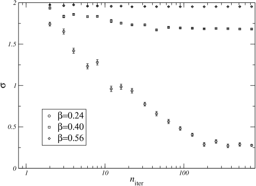
Figure 1: Surface tension $\sigma$ versus the number of iterations $n_{\rm iter.}$ for three different temperatures: $\beta=0.24$, $\beta=0.40$ and $\beta=0.56$ from bottom to top. The lattice size is $L=16$. Error bars on the data correspond to statistical errors.

The surface tension is calculated according to the method presented in section 2. Estimates of the surface tension for an increasing number of iterations $n_{\rm iter.}$ are plotted on figure 1. The number of experiments is kept fixed to the value $n_{\rm exp.}=1000$ which means that rare events with a probability smaller than $1/n_{\rm exp.}=10^{-3}$ are not correctly sampled. The figure shows two regimes. When the number of iterations is large $n_{\rm niter}>n_{\rm iter}^{\rm opt.}$, the estimates display a plateau. The amplitude of the fluctuations around the value of this plateau is of the same order of magnitude than the error bars. In contradistinction, the estimates display a systematic deviation when the number of iterations is small $n_{\rm niter}<n_{\rm iter}^{\rm opt.}$. The data indicate a deviation proportional to $\ln{1\over n_{\rm niter}}$. The contribution of the rare events are larger than the statistical errors and cannot be neglected. The cross-over between the two regimes depends on the temperature. Surprisingly, it does not depend much on the lattice size.

We have also tried to estimate the surface tension using the width $\sigma_{W_{S}}^{2}=\langle W_{S}^{2}\rangle-\langle W_{S}\rangle^{2}$ of the probability distribution of the entropic work. These distributions are indeed close to Gaussian distributions so the Jarzynski relation reads

$$\langle e^{-W_{S}}\rangle={1\over\sqrt{2\pi\sigma_{W_{S}}^{2}}}\int e^{-W_{S}-(W_{S}-\langle W_{S}\rangle)^{2}/2\sigma_{W_{S}}^{2}}dW_{S}\Leftrightarrow\ \Delta(\beta F)=\langle W_{S}\rangle-{\sigma_{W_{S}}^{2}\over 2}$$ (9)

The estimates of the surface tension are compatible with those obtained using the Jarzynski relation $(\ref{eqJarzynski3})$ but the error bars are larger. As a consequence, we will not consider this estimate in the following.

Our numerical data of the surface tension are presented on figures 2 (PBC) and 3 (FBC). The few points with large error bars on figure 3 correspond to small systems at temperatures higher than the finite-size “critical” temperature $T_{c}(L)$. The system is thus already in the paramagnetic phase and the interface disappears. No order-order surface tension can then be given. In contradistinction to the two-dimensional case, the surface tension displays larger finite-size corrections with FBC. The data have been extrapolated to the thermodynamic limit using the ansatz:

$$\sigma(L)=\sigma(\infty)+{c_{1}\over L^{2}}+{c_{2}\over L^{4}}$$ (10)

for PBC and

$$\sigma(L)=\sigma(\infty)+{d_{1}\over L}+{d_{2}\over L^{2}}$$ (11)

for FBC. The error bars on the value $\sigma(\infty)$ take into account both the errors on the data and due to the fit. The figure 4 gives an example of this extrapolation for three different temperatures. While the whole range of lattice sizes $L$ are well reproduced by the ansatz (10) for PBC, the two smallest lattice sizes ($L=4$ and $L=6$) cannot be taken into account by (11) for FBC and have been discarded. The extrapolated value $\sigma(\infty)$ of the surface tension can be compared in figures (2) and (3) to the 17th-order low-temperature expansion (see [29] for the coefficients) and to large-scale Monte Carlo simulations [29]. Our data are perfectly compatible to the latter apart from a small disagreement for FBC at temperatures close to the critical point. The too simple ansatz (11) may be responsible for this disagreement.

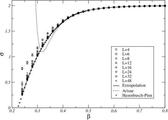
Figure 2: Numerical estimates of the surface tension of the 3D Ising model with respect to the inverse temperature $\beta$ for periodic boundary conditions.

Figure 3: Numerical estimates of the surface tension of the 3D Ising model with respect to the inverse temperature $\beta$ for free boundary conditions.

Figure 4: Extrapolation of the surface tension for three different temperatures. The solid curves correspond to periodic boundary conditions and the dashed ones to free boundary conditions.

4 Discussion and conclusions

We have discussed a Jarzynski relation generalized to temperature changes. Its derivation is limited to Markovian dynamics since the interaction with the bath is properly taken into account only in this case. We have then presented a modified version of the usual algorithm allowing for the computation of the surface tension by Monte Carlo simulations where the Jarzynski relation replaces thermodynamic perturbation. The approach has been tested in the case of the 3D Ising model. Despite the common belief that rare events prevent the application of Jarzynski relation, the method is efficient because the transformation does not bring the system far from equilibrium. This is possible because the method uses initial and final states not very different. Basically, the final state display thermal fluctuations while the initial state is almost the ground state. But in both cases, two ferromagnetic phases are separated by an interface. In contradistinction to other algorithms, the interface is not created during the transformation. Moreover, we use cluster algorithms. Their relaxation times are much smaller than the usual Metropolis algorithm and allows the final state to be close to equilibrium. The systematic deviation due to an insufficient sampling of the rare events that dominates the average $\langle e^{-W_{S}}\rangle$ has been shown to be negligible compared to statistical errors for a reasonable number of iterations. Our aim was only to prove the usefulness of the Jarzynski relation despite the fact that rare events play an important role and not to add a 6th or 7th new digit to the estimates of the surface tension that can be found in the literature. The computational effort we devoted to the calculation is much smaller (around 100 times) than that of ref. [29] for instance. For $\beta=0.45$ and $L=32$, our estimate of the surface tension is $1.8316(4)$ while Hasenbusch et al. obtained a much accurate estimate: $1.831368(5)$. However, they only calculated numerically the difference $F(\beta=0.45)-F(\beta_{i}=0.515)$ and then used the 17th-order low-temperature expansion estimate of $F(\beta=0.515)$ to obtain the surface tension. We calculated numerically the difference $F(\beta=0.45)-F(\beta_{i}=2)$ and estimated $F(\beta_{i}=2)$ as the $T=0$ ground-state free energy. By starting with a much temperature, we do not need the 17th-order low-temperature expansion to calculate the surface tension.

The main drawback of our approach is that the convergence of estimates of the free energy obtained by the Jarzynski relation is not well understood yet. We cannot give any recipe to adjust the three parameters $N,n_{\rm iter.},n_{\rm exp.}$ to obtain the best convergence. Research efforts in this direction are highly desirable.

One can imagine other protocols based on the Jarzynski relation to estimate the surface tension. One can start first with a strong homogeneous magnetic field on the up and down boundaries to force the system in the ferromagnetic state. Then one of these magnetic fields is reversed to favor the appearance of the interface. By recording the work while the magnetic field is reversed, the free energy could be estimated using the more usual Jarzynski relation (1). However, the convergence may not be as good because an interface has to be created during the magnetic field reversal. In the approach based on variation of the temperature, this interface is already present in the initial state.

The relation (22) may be useful even in the case of the measurement of the difference of the free energies of two equilibrium states at the same temperature. If these two states are separated by a free energy barrier, the relation (22) allows first to increase the temperature so that the system can pass the barrier and then to decrease the temperature down to its initial value.

Appendix: derivation of the Jarzynski relation

We shall derive the Jarzynski relation along the lines of the derivation given in the appendix of [2]. Let us denote $\vec{\sigma}$ the microscopic states of the system, i.e. the spin configurations in the case of the Ising model. We shall assume that the dynamics of the system is Markovian and is governed by the master equation

$$\wp(\vec{\sigma},t+1)=\sum_{\vec{\sigma}^{\prime}}\wp(\vec{\sigma}^{\prime},t)W_{\beta(t),h(t)}(\vec{\sigma}^{\prime}\rightarrow\vec{\sigma})$$ (12)

where $\wp(\vec{\sigma},t)$ is the probability to find the system in the state $\vec{\sigma}$ at time $t$ and $W_{\beta(t),h(t)}(\vec{\sigma}\rightarrow\vec{\sigma}^{\prime})$ is the transition rate per time step from the state $\vec{\sigma}$ to the state $\vec{\sigma}^{\prime}$. The transition rates take into account the interaction of the system with an heat bath in an effective manner. They depend on the temperature $T=1/k_{B}\beta$ of the bath and on an external parameter $h$, for instance the magnetic field. The master equation is equivalent to the Bayes relation which means that the transition rates are conditional probabilities: $W_{\beta(t),h(t)}(\vec{\sigma}\rightarrow\vec{\sigma}^{\prime})=\wp(\vec{\sigma}^{\prime},t+1|\vec{\sigma},t)$. As a consequence, the transition rates satisfy the condition

$$\sum_{\vec{\sigma}^{\prime}}W_{\beta,h}(\vec{\sigma}\rightarrow\vec{\sigma}^{\prime})=1$$ (13)

When $\beta$ and $h$ are kept constant, the system is expected to evolve towards the Boltzmann equilibrium distribution

$$\pi_{\beta,h}(\vec{\sigma})={1\over{\cal Z}_{\beta,h}}e^{-\beta(E(\vec{\sigma})-hM(\vec{\sigma}))}$$ (14)

where $M$ is the extensive quantity associated to the control parameter $h$ (for instance the magnetization when $h$ is the magnetic field). The equilibrium distribution satisfies the stationarity condition

$$\pi_{\beta,h}(\vec{\sigma})=\sum_{\vec{\sigma}^{\prime}}\pi_{\beta,h}(\vec{\sigma}^{\prime})W_{\beta,h}(\vec{\sigma}^{\prime}\rightarrow\vec{\sigma})$$ (15)

For convenience one imposes the more restrictive condition of detailed balance

$$\pi_{\beta,h}(\vec{\sigma})W_{\beta,h}(\vec{\sigma}\rightarrow\vec{\sigma}^{\prime})=\pi_{\beta,h}(\vec{\sigma}^{\prime})W_{\beta,h}(\vec{\sigma}^{\prime}\rightarrow\vec{\sigma})$$ (16)

that leads to (15) when using the condition (13).

At time $t=t_{i}$ the system is thermalized with a bath at the temperature $1/k_{B}\beta(t_{i})$ and external parameter $h(t_{i})$, i.e. $\wp(\vec{\sigma},t_{i})=\pi_{\beta(t_{i}),h(t_{i})}(\vec{\sigma})$. The temperature and the external parameter are then varied and the quantity

$$\langle X(t_{i},t_{f})\rangle=\langle e^{-\sum_{t=t_{i}}^{t_{f}-1}(\Delta_{t}\beta E(\vec{\sigma}(t))-\Delta_{t}(\beta h)M(\vec{\sigma}(t)))}\rangle$$ (17)

is measured. The brackets $\langle\ldots\rangle$ denotes an average over all possible histories of the system between $t_{i}$ and $t_{f}$. We have introduced the notations $\Delta_{t}\beta=\beta(t+1)-\beta(t)$ and $\Delta_{t}(\beta h)=\beta(t+1)h(t+1)-\beta(t)h(t)$. Following Jarzynski [2], each time step consists into two substeps. First the temperature and the external parameter are changed by an amount $\Delta_{t}\beta$ and $\Delta_{t}h$. The latter induces a work $W=-\Delta_{t}hM$. In the second substep, the master equation is iterated once so that the system makes a transition to a new state $\vec{\sigma}(t+1)$ with the conditional probability $W_{\beta(t+1),h(t+1)}(\vec{\sigma}(t)\rightarrow\vec{\sigma}(t+1))$. The energy change $E(\vec{\sigma}(t+1))-E(\vec{\sigma}(t))$ corresponds to the heat exchanged with the heat bath. Rewriting $X(t_{i},t_{f})$ using the equilibrium probability (14) as

$$X(t_{i},t_{f})=\prod_{t=t_{i}}^{t_{f}-1}{{\cal Z}_{\beta(t+1),h(t+1)}\pi_{\beta(t+1),h(t+1)}(\vec{\sigma}(t))\over{\cal Z}_{\beta(t),h(t)}\pi_{\beta(t),h(t)}(\vec{\sigma}(t))},$$ (18)

the average (17) reads

$$\langle X(t_{i},t_{f})\rangle = \sum_{\{\vec{\sigma}(t)\}}\pi_{\beta(t_{i}),h(t_{i})}(\vec{\sigma}(t_{i}))\prod_{t=t_{i}}^{t_{f}-1}\Big{[}{{\cal Z}_{\beta(t+1),h(t+1)}\pi_{\beta(t+1),h(t+1)}(\vec{\sigma}(t))\over{\cal Z}_{\beta(t),h(t)}\pi_{\beta(t),h(t)}(\vec{\sigma}(t))}\Big{.}$$ (19)

$$\Big{.}\hskip 110.00017pt\times W_{\beta(t+1),h(t+1)}(\vec{\sigma}(t)\rightarrow\vec{\sigma}(t+1))\Big{]}$$

All but two partition functions cancel. Using the detailed balance condition (16), one obtains

$$\langle X(t_{i},t_{f})\rangle = {{\cal Z}_{\beta(t_{f}),h(t_{f})}\over{\cal Z}_{\beta(t_{i}),h(t_{i})}}\sum_{\{\vec{\sigma}(t)\}}\pi_{\beta(t_{i}),h(t_{i})}(\vec{\sigma}(t_{i}))\prod_{t=t_{i}}^{t_{f}-1}\Big{[}{\pi_{\beta(t+1),h(t+1)}(\vec{\sigma}(t+1))\over\pi_{\beta(t),h(t)}(\vec{\sigma}(t))}\Big{.}$$

$$\Big{.}\hskip 110.00017pt\times W_{\beta(t+1),h(t+1)}(\vec{\sigma}(t+1)\rightarrow\vec{\sigma}(t))\Big{]}$$

Now all but one equilibrium probabilities cancel and one gets

$$\langle X(t_{i},t_{f})\rangle={{\cal Z}_{\beta(t_{f}),h(t_{f})}\over{\cal Z}_{\beta(t_{i}),h(t_{i})}}\sum_{\{\vec{\sigma}(t)\}}\pi_{\beta(t_{f}),h(t_{f})}(\vec{\sigma}(t_{f}))\prod_{t=t_{i}}^{t_{f}-1}W_{\beta(t+1),h(t+1)}(\vec{\sigma}(t+1)\rightarrow\vec{\sigma}(t))$$ (21)

Finally, the sum over histories of the system is easily shown to be equal to 1 using equation (15). Introducing the definition of the free-energy $F(\beta,h)=-\beta^{-1}\ln{\cal Z}_{\beta,h}$, one obtains the Jarzynski relation

$$\langle e^{-\sum_{t=t_{i}}^{t_{f}-1}(\Delta_{t}\beta E(\vec{\sigma}(t))-\Delta_{t}(\beta h)M(\vec{\sigma}(t)))}\rangle=e^{-[\beta(t_{f})F(\beta(t_{f}),h(t_{f}))-\beta(t_{i})F(\beta(t_{i}),h(t_{i}))]}$$ (22)

In this paper, we restrict ourselves to the case $h=0$, i.e.

$$\langle e^{-\sum_{t=t_{i}}^{t_{f}-1}\Delta_{t}\beta E(\vec{\sigma}(t))}\rangle=e^{-[\beta(t_{f})F(\beta(t_{f}))-\beta(t_{i})F(\beta(t_{i}))]}$$ (23)

The relation (22) is appropriate for Monte Carlo simulations since the time is discrete. The demonstration given by Jarzynski in the case of a Markovian process in continuous time can also be extended to a varying temperature [2]. It leads to

$$\langle e^{-\int_{t_{i}}^{t_{f}}[\dot{\beta}U(\vec{\sigma}(t))-\beta\dot{h}M(\vec{\sigma}(t))]dt}\rangle=e^{-[\beta(t)F(\beta(t),h(t))]_{t_{i}}^{t_{f}}}$$ (24)

where $U(\vec{\sigma}(t))=E(\vec{\sigma}(t))-h(t)M(\vec{\sigma}(t))$ is the total energy of the system in the state $\vec{\sigma}(t)$.

References

- [1] Jarzynski C. (1997) Phys. Rev. Lett. 78, 2690
- [2] Jarzynski C. (1997) Phys. Rev. E 56, 5018.
- [3] Crooks G.E. (1999) Excursions in Statistical Dynamics, Dissertation at the univ. of California at Berkeley (unpublished)
- [4] Neal R.M. (2001) Statistics and Computing 11, 125.
- [5] Chen S., Ferrenberg A.M. and Landau D.P. (1995) Phys. Rev. E 52, 1377.
- [6] Janke W. and Villanova R. (1997) Nucl. Phys. B 489, 679.
- [7] Provata A., Prassas D. and Theodorou D.N. (1997) J. Chem. Phys. 107 5125.
- [8] Jain T.S. and de Pablo J.J. (2003) J. Chem. Phys. 118, 4226.
- [9] Huang S., Potvin J., Rebbi C. and Sanielevici S. (1990) Phys. Rev. D 42, 2864.
- [10] Grossmann B., Laursen M.L., Trappenberg T. and Wiese U.J. (1992) Phys. Lett. B 293, 175.
- [11] Alves N.A. (1992) Phys. Rev. D 46, 3678.
- [12] Brower R., Huang S., Potvin J. and Rebbi C. (1992) Phys. Rev. D 46, 2703.
- [13] Hackel M., Faber M., Markum H. and Müller M. (1992) Phys. Rev. D 46, 5648.
- [14] Papa A. (1994) Phys. Lett. B 420, 91.
- [15] Caselle M., Hasenbusch M. and Panero M. (2006) JHEP 0603, 084.
- [16] Berg B.A. and Neuhaus T. (1992) Phys. Rev. Lett. 68, 9
- [17] Binder K. (1982) Phys. Rev. A 25, 1699.
- [18] de Forcrand P., d’Ellia M. and Pepe M. (2001) Phys. Rev. Lett. 86, 1438.
- [19] Pepe M. and de Forcrand P. (2002) Nucl. Phys. Proc. Suppl. 106, 914.
- [20] de Forcrand P. and Noth D. (2005) Phys. Rev. D 72, 114501.
- [21] de Forcrand P., Lucini B. and Noth D. (2005) PoS LAT2005 323
- [22] Ising E. (1925) Zeits. f. Physik 31, 253.
- [23] Bennett C.H. (1976) J. Comp. Phys. 22, 245.
- [24] Blöte H.W.J., Shchur L.N. and Talapov A.L. (1999) Int. J. Mod. Phys. C 10, 1137.
- [25] Gore J., Ritort F. and Bustamante C. (2003) Proc. Natl. Acad. Sci. (USA) 100, 12564.
- [26] Jarzynski C. (2006) Phys. Rev. E 73, 046105.
- [27] Hasenbusch M. and Meyer S. (1991) Phys. Rev. Lett. 66, 530.
- [28] Swendsen R.H. and Wang J.S. (1987) Phys. Rev. Lett. 58, 86.
- [29] Hasenbusch M. and Pinn K. (1994) Physica A 203 189