Quantum disordering of the $111$ state and the compressible–incompressible transition in quantum Hall bilayer systems

Abstract

We systematically discuss properties of quantum disordered states of the quantum Hall bilayer at $\nu_{T}=1$. For one of them, so-called vortex metal state, we find ODLRO (off-diagonal long-range order) of algebraic kind, and derive its transport properties. It is shown that this state is relevant for the explanation of the “imperfect” superfluid behavior, and persistent intercorrelations, for large distances between layers, that were found in experiments.

I Introduction

Electrons in quantum Hall bilayer systems at total filling factor $\nu_{T}=1$ naturally correlate in two different ways due to Pauli principle and Coulomb interaction. If the layers are sufficiently far apart, dominant correlations would be those of intralayer kind because electrons in one layer are unable to sense what is taking place in the opposite layer. This does not hold, however, in the limit of small layer separation. Instead, with decreasing $d/l_{B}$, the ratio of the distance between layers to the magnetic length, the correlations between electrons in different layers gain strength and begin to compete with intralayer correlations. It is the interplay of those two kinds of correlations that we focus on in this paper.

For the case of prevalent interlayer correlations, there are already a few theoretical models at hand which provide a satisfactory description: $111$-state given by Halperin’s halperin $111$ wavefunction $\Psi_{111}=\prod_{i<j}(z_{i\uparrow}-z_{j\uparrow})\prod_{k<l}(z_{k\downarrow}-z_{l\downarrow})\prod_{m,n}(z_{m\uparrow}-z_{n\downarrow}),$ quantum Hall ferromagnet, kmoon condensate of excitons macdonald or composite bosons. stanic Nevertheless, both theoretically and experimentally, it is evident that with increasing $d/l_{B}$ a quantum disordering of this state is bound to take place. For example, the tunneling peak observed by Spielman et al. spielman is indeed sharp and pronounced, but its nature is more that of a resonance than of the speculated Josephson effect, while the temperature dependences of Hall and longitudinal resistance in experiments of Kellogg et al. kellogg and Tutuc et al. tutuc do not provide support to the predicted Berezinskii-Kosterlitz-Thouless (BKT) scenario of a bilayer finite temperature phase transition. kmoon Deeper understanding of the regime $d\sim l_{B}$ is therefore an important, open problem in the physics of quantum Hall bilayers and strongly correlated electron systems in general.

Hereinafter we present some results which pertain to quantum disordering that is believed to take place in the quantum Hall bilayer at $\nu_{T}=1$. The ground state at $d=0$ is a Bose condensate well-described by $111$-wavefunction due to Halperin, while the low-lying excitations are composite bosons i.e. electrons dressed with one quantum of magnetic flux. stanic The idea of disordering that we employ is to allow the formation of composite fermions (i.e. electrons dressed with two quanta of magnetic flux) that coexist with composite bosons. srm03 There are two ways to introduce composite fermions into the Bose condensate and this will be explained in Sec. II. We then pursue a phenomenological Chern-Simons transport theory à la Drude in order to examine the elementary predictions of those two model states. In Sec. III we arrive at an effective gauge theory for both cases. This enables us to calculate the correlation functions, modes of low-lying excitations and characteristic off-diagonal long-range order (ODLRO). We will be primarily interested in the pseudospin channel of these states. In one of those, the so-called vortex metal state that we believe may appear in the bilayer at larger $d/l_{B}$ as a manifestation of increasing intracorrelations, we derive an algebraic ODLRO. In Sec. IV we focus on the incompressible region and the crossover around the critical layer separation. We will argue that our field-theoretical, homogeneous picture in fact suggests that vortex metal, if relevant for the strongly-coupled, incompressible region, may appear only localized, in form of islands in the background of the superfluid state for smaller $d/l_{B}$. In Sec. V we give a more thorough analysis of the experiments on bilayer, addressing especially the compressible, weakly-coupled region, and the question of persistent intercorrelations kelloggdrag in the framework of the vortex metal state. Sec. VI is devoted to discussion and conclusion. For the sake of clarity and in order to make the text self-contained, some of the known results srm03 ; milica-preprint will be re-derived in this paper.

II Trial wavefunctions for the bilayer

Building on Laughlin’s proposal for the wavefunction of a single quantum Hall layer, laughlin-orig the construction of Rezayi-Read wavefunction rezayi-read for $\nu=1/2$ and Halperin’s $111$-wavefunction for bilayer, halperin we may formally imagine that there are two species of electrons in each layer ($z,w$) which are all mutually correlated through intracorrelations (within the same layer) and intercorrelations (between opposite layers), Fig. 1.

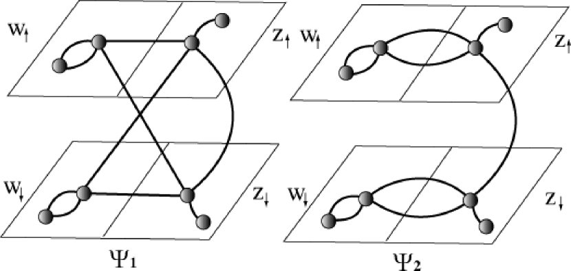
Figure 1: Correlations between electrons in two layers.

Starting from the $111$-function of the Bose condensate, we will minimally deform it in order to include the composite fermions. Given that each particle binds the same number of flux quanta and taking Pauli principle into account, this becomes a combinatorial problem with two solutions. In the first case:

$$\Psi_{1}=\mathcal{P}\mathcal{A}\{\prod_{i<j}(z_{i\uparrow}-z_{j\uparrow})\prod_{k<l}(z_{k\downarrow}-z_{l\downarrow})\prod_{p,q}(z_{p\uparrow}-z_{q\downarrow})$$

$$\times\Phi_{f}(w_{\uparrow},\overline{w}_{\uparrow})\prod_{i<j}(w_{i\uparrow}-w_{j\uparrow})^{2}$$

$$\times\Phi_{f}(w_{\downarrow},\overline{w}_{\downarrow})\prod_{k<l}(w_{k\downarrow}-w_{l\downarrow})^{2}$$

$$\times\prod_{i,j}(z_{i\uparrow}-w_{j\uparrow})\prod_{k,l}(z_{k\uparrow}-w_{l\downarrow})$$

$$\times\prod_{p,q}(z_{p,\downarrow}-w_{q,\uparrow})\prod_{m,n}(z_{m\downarrow}-w_{n\downarrow})\}.$$ (1)

The first line in this formula can be recognized as $111$-function, followed by two $\nu=1/2$ separate layers ($\Phi_{f}$’s denote the Slater determinants of free composite fermions), while the last two lines stem from the flux-particle constraint (all these correlations are depicted on the left hand side of Fig. 1). $\mathcal{P},\mathcal{A}$ denote projection to the lowest Landau level (LLL) and fermionic antisymmetrization (independently for each layer), respectively. In thermodynamic limit, the relation between the number of particles and flux quanta reads milica-preprint :

$$N_{\Phi}=N_{b\uparrow}+N_{b\downarrow}+N_{f\uparrow}+N_{f\downarrow}$$

$$=2N_{f\uparrow}+N_{b\uparrow}+N_{b\downarrow}=2N_{f\downarrow}+N_{b\uparrow}+N_{b\downarrow}.$$ (2)

$N_{\Phi}$ is the number of flux quanta through the system, and $N_{b\sigma}$ and $N_{f\sigma}$ are the number of bosons and fermions inside the layer $\sigma$ respectively; $\sigma=\uparrow,\downarrow$ is the layer index. Eq. (II) enforces an additional constraint $N_{f\uparrow}=N_{f\downarrow}.$ Therefore, the number of fermions is balanced in two layers, while boson numbers are not subject to any such constraint. This fact is important because of the broken symmetry of spontaneous interlayer phase coherence in the $111$-state, which demands nonconservation of $N_{b\uparrow}-N_{b\downarrow}$. Although we work in a fixed (relative) number representation (allowed in a broken symmetry case), to account for a broken symmetry situation we need to have a possibility of unconstrained relative number of bosons. Then a superposition of the wavefunctions of the form in Eq. (II) would lead to the usual representation.

In the second case which is expected to describe dominant intracorrelations, fermions bind exclusively within the layer they belong to (right side of Fig. 1) and the corresponding wavefunction is:

$$\Psi_{2}=\mathcal{P}\mathcal{A}\{\prod_{i<j}(z_{i\uparrow}-z_{j\uparrow})\prod_{k<l}(z_{k\downarrow}-z_{l\downarrow})\prod_{p,q}(z_{p\uparrow}-z_{q\downarrow})$$

$$\times\Phi_{f}(w_{\uparrow},\overline{w}_{\uparrow})\prod_{i<j}(w_{i\uparrow}-w_{j\uparrow})^{2}$$

$$\times\Phi_{f}(w_{\downarrow},\overline{w}_{\downarrow})\prod_{k<l}(w_{k\downarrow}-w_{l\downarrow})^{2}$$

$$\times\prod_{i,j}(z_{i\uparrow}-w_{j\uparrow})^{2}\prod_{k,l}(z_{k\downarrow}-w_{l\downarrow})^{2}\}.$$ (3)

In this case, the flux-particle relation milica-preprint is:

$$N_{\Phi}=2N_{f\uparrow}+2N_{b\uparrow}=2N_{f\downarrow}+2N_{b\downarrow}$$

$$=2N_{f\uparrow}+N_{b\uparrow}+N_{b\downarrow}=2N_{f\downarrow}+N_{b\uparrow}+N_{b\downarrow},$$ (4)

implying that both fermion and boson numbers must be balanced: $N_{f\uparrow}=N_{f\downarrow},N_{b\uparrow}=N_{b\downarrow}.$

In Ref. srm03, the authors numerically calculated the overlap of $\Psi_{1}$ with the exact ground state wavefunction for a system of $5$ electrons in each layer with varying $d/l_{B}$. Their results seem to demonstrate convincingly that (at least for small systems) the approach with trial wavefunctions that interpolate between two well-established limits, namely those of $111$-state and decoupled $\nu=1/2$ layers, is not only an artificial mathematical construction but corresponds to physical reality. Despite the fact that the number of electrons in this simulation is certainly well below the thermodynamic limit, the fact that the overlaps between $\Psi_{1}$ and the exact ground state display peaks very close to $1$ at small $d/l_{B}$ provides confidence in the choice of wavefunction $\Psi_{1}$ (at least for small $d/l_{B}$).

If there is a phase separation in between the sea of composite bosons and composite fermions, the phase transition will be of the first order. Such a scenario is launched in Ref. stern-halperin, , where the authors imagine static, isolated regions of incoherent phase inside $111$ phase. Although this model correctly explains some of the observed phenomena (e.g. semicircle law), the persistence of intercorrelations in the weakly-coupled, compressible regime kelloggdrag which gradually die out suggests a continuous transition. Such a possibility is naturally present in the picture of composite boson-composite fermion mixture.

A transport theory of Drude kind can be easily formulated srm03 if we consider that composite fermions bind two quanta of magnetic flux, unlike composite bosons which bind only one quantum of magnetic flux. As long as we remain in the RPA approximation, they can all be treated as free particles moving in the presence of the effective field which is given by the sum of the external and self-consistently induced electric field. In the first case ($\Psi_{1}$), the effective field as seen by particles in the layer $\sigma$ is:

$$\mathcal{E}_{f}^{\sigma}=\mathbf{E}^{\sigma}-2\mathbf{\epsilon}\mathbf{J}_{f}^{\sigma}-\mathbf{\epsilon}(\mathbf{J}_{b}^{1}+\mathbf{J}_{b}^{2}),$$ (5)

$$\mathcal{E}_{b}^{\sigma}=\mathbf{E}^{\sigma}-\mathbf{\epsilon}(\mathbf{J}_{b}^{1}+\mathbf{J}_{b}^{2}+\mathbf{J}_{f}^{1}+\mathbf{J}_{f}^{2}),$$ (6)

where $\mathbf{J}_{f(b)}^{\sigma}$ denote Fermi- and Bose-currents in the layer $\sigma$ and $\mathbf{\epsilon}=\left[\begin{array}[]{rrr}0&\delta\\ -\delta&0\\ \end{array}\right]$, $\delta=\frac{h}{e^{2}}$. Transport equations are:

$$\mathcal{E}_{f(b)}^{\sigma}=\rho_{f(b)}^{\sigma}\mathbf{J}_{f(b)}^{\sigma}$$ (7)

and, as required by symmetry, $\rho_{f(b)}^{1}=\rho_{f(b)}^{2}$, while the total current is given by $\mathbf{J}^{\sigma}=\mathbf{J}_{b}^{\sigma}+\mathbf{J}_{f}^{\sigma}.$ We define single layer resistance ($\rho^{11}$) and drag resistance ($\rho^{D}$) as follows::

$$\mathbf{E}^{1}=\rho^{11}\mathbf{J}^{1},$$ (8)

$$\mathbf{E}^{2}=\rho^{D}\mathbf{J}^{1}.$$ (9)

When both layers have the same filling, $\nu_{1}=\nu_{2}=1/2$, tensors $\rho_{b},\rho_{f}$ are diagonal (because the composite particles are in zero net field): $\rho_{b}=\verb"diag"\left[\rho_{bxx},\rho_{bxx}\right]$, $\rho_{f}=\verb"diag"\left[\rho_{fxx},\rho_{fxx}\right],$ and in the case of drag we have in addition $\mathbf{J}^{2}=0,\mathbf{J}^{1}-$finite. Then from Eqs. (5)-(9) via elementary algebraic manipulations we obtain:

$$\rho^{11}=1/2\{\left[\rho_{b}^{-1}+\rho_{f}^{-1}\right]^{-1}+2\epsilon$$

$$+\left[(\rho_{f}+2\epsilon)^{-1}+\rho_{b}^{-1}\right]^{-1}\},$$ (10)

$$\rho^{D}=1/2\{\left[\rho_{b}^{-1}+\rho_{f}^{-1}\right]^{-1}+2\epsilon$$

$$-\left[(\rho_{f}+2\epsilon)^{-1}+\rho_{b}^{-1}\right]^{-1}\},$$ (11)

or, in terms of matrix elements:

$$\rho_{xx}^{D}=-\frac{2\rho_{bxx}^{2}\delta^{2}}{(\rho_{bxx}+\rho_{fxx})^{3}+4(\rho_{bxx}+\rho_{fxx})\delta^{2}},$$ (12)

$$\rho_{xy}^{D}=\frac{\delta(2\rho_{bxx}\rho_{fxx}+\rho_{fxx}^{2}+4\delta^{2})}{\rho_{bxx}^{2}+2\rho_{bxx}\rho_{fxx}+\rho_{fxx}^{2}+4\delta^{2}},$$ (13)

$$\rho_{xx}^{11}=\frac{2\rho_{bxx}^{2}\delta^{2}}{(\rho_{bxx}+\rho_{fxx})^{3}+4(\rho_{bxx}+\rho_{fxx})\delta^{2}}$$

$$+\frac{\rho_{bxx}\rho_{fxx}}{(\rho_{bxx}+\rho_{fxx})}.$$ (14)

Formulas in Eqs. (12)-(II) include parameters $\delta$, $\rho_{bxx}$ and $\rho_{fxx}$, the last two being free parameters about which nothing can be said a priori. This prompted Simon et al. srm03 to reason as follows. At large $d/l_{B}$ the number of composite bosons is small because the condensate is broken and $\rho_{bxx}$ is large compared to $\delta$, which is the typical Hall resistance. On the other hand, from the experiments willett we know that for large $d/l_{B}$ holds $\rho_{fxx}\ll\delta$. Furthermore, even as $d/l_{B}$ is decreased, we expect $\rho_{fxx}$ to increase only slightly. srm03 All in all, for large $d/l_{B}$ they assume $\rho_{bxx}\gg\delta\gg\rho_{fxx}$, and if in addition we allow $\rho_{bxx}\rho_{fxx}\ll\delta^{2}$, asymptotically we obtain:

$$\rho_{xx}^{D}\approx-\frac{2\delta^{2}}{\rho_{bxx}},$$ (15)

$$\rho_{xy}^{D}\approx 4\delta(\frac{\delta}{\rho_{bxx}})^{2},$$ (16)

$$|\rho_{xx}^{11}|\approx|\rho_{xx}^{D}|.$$ (17)

Semicircle law follows directly from the previous formulas:

$$(\rho_{xx}^{D})^{2}+(\rho_{xy}^{D}-\frac{\delta}{2})^{2}\approx(\frac{\delta}{2})^{2},$$ (18)

in agreement with Ref. stern-halperin, (semicircle law is of general validity for twocomponent systems in two dimensions and it serves us as a crucial test for the the line of reasoning quoted above, which may at first sound somewhat naïve).

In the opposite limit (when $d/l_{B}$ is reduced), $\rho_{bxx}\ll\rho_{fxx}\ll\delta$, because $\rho_{bxx}$ drops as a result of Bose condensation srm03 . When $\rho_{bxx}\rightarrow 0$ we obtain the quantization of Coulomb drag:

$$\rho_{xy}^{D}\approx\delta,$$ (19)

$$\rho_{xx}^{D}\longrightarrow 0,$$ (20)

as measured by Kellogg et al. kellogg

Let us return now to the case of dominant intracorrelations, the vortex metal state milica-preprint represented by Eq. (II). From Fig. 1 the formulas for effective fields are modified into:

$$\mathcal{E}_{f}^{\sigma}=\mathbf{E}^{\sigma}-2\mathbf{\epsilon}\mathbf{J}_{f}^{\sigma}-2\mathbf{\epsilon}\mathbf{J}_{b}^{\sigma},$$ (21)

$$\mathcal{E}_{b}^{\sigma}=\mathbf{E}^{\sigma}-\mathbf{\epsilon}(\mathbf{J}_{b}^{1}+\mathbf{J}_{b}^{2}+2\mathbf{J}_{f}^{\sigma}),$$ (22)

and the analogous calculation yields the resistivity tensors:

$$\rho^{11}=\frac{1}{2}\{\left[\rho_{b}^{-1}+\rho_{f}^{-1}\right]^{-1}+2\epsilon$$

$$+\left[(\rho_{b}-2\epsilon)^{-1}+\rho_{f}^{-1}\right]^{-1}\left[(\rho_{b}-2\epsilon)^{-1}\rho_{b}+2\rho_{f}^{-1}\epsilon\right])\},$$ (23)

$$\rho^{D}=\frac{1}{2}\{\left[\rho_{b}^{-1}+\rho_{f}^{-1}\right]^{-1}+2\epsilon$$

$$-\left[(\rho_{b}-2\epsilon)^{-1}+\rho_{f}^{-1}\right]^{-1}\left[(\rho_{b}-2\epsilon)^{-1}\rho_{b}+2\rho_{f}^{-1}\epsilon\right]\}.$$ (24)

The matrix elements of these tensors are:

$$\rho_{xx}^{D}=-\frac{2\rho_{fxx}^{2}\delta^{2}}{(\rho_{bxx}+\rho_{fxx})^{3}+4(\rho_{bxx}+\rho_{fxx})\delta^{2}},$$ (25)

$$\rho_{xy}^{D}=\frac{\rho_{fxx}^{2}\delta}{(\rho_{fxx}+\rho_{bxx})^{2}+4\delta^{2}},$$ (26)

$$\rho_{xx}^{11}=\frac{2\rho_{fxx}^{2}\delta^{2}}{(\rho_{bxx}+\rho_{fxx})^{3}+4(\rho_{bxx}+\rho_{fxx})\delta^{2}}$$

$$+\frac{\rho_{bxx}\rho_{fxx}}{(\rho_{bxx}+\rho_{fxx})}.$$ (27)

In this case as well, there are two physically significant limits depending on the assumptions for the values of $\rho_{bxx},\rho_{fxx}$. In the case when $\rho_{bxx}\ll\rho_{fxx}\ll\delta$:

$$\rho_{xx}^{D}\approx-\frac{\rho_{fxx}}{2},$$ (28)

$$\rho_{xy}^{D}\approx\frac{1}{4}\frac{\rho_{fxx}^{2}}{\delta},$$ (29)

$$\rho_{xx}^{11}\approx\frac{\rho_{fxx}}{2},$$ (30)

and the semicircle law follows, Eq. (18), whereas $|\rho_{xx}^{D}|=|\rho_{xx}^{11}|.$ Similarly, in the regime $\rho_{bxx}\ll\delta\ll\rho_{fxx}$ we deduce the quantization of Coulomb drag, Eqs. (19)-(20).

We emphasize that these two limits are different from those in Simon et al. srm03 For example, the semicircle law was derived assuming that $\rho_{bxx}$ is small (which is exactly the opposite situation to the one in Ref. srm03, ), while $\rho_{fxx}$ is not necessarily small with respect to $\delta$. As noted in the first case above, the exact values for $\rho_{bxx},\rho_{fxx}$ are in fact unknown and this prevents us from discriminating between the different proposed limits. In other words, we cannot say which one of the proposed limits is plausible - the analysis above serves us only to conclude that each of the two composite boson-composite fermion mixed states are able (with certain assumptions) to reproduce the phenomenology of drag experiments.

III Chern-Simons theory for bilayer

Encouraged by the preliminary analysis from the previous section, we will pursue the idea of composite boson-composite fermion mixture further by formulating an example of Chern-Simons (CS) field theory which can contain wavefunctions $\Psi_{1},\Psi_{2}$ as ground states. We do not embark on such a task only for the sake of completeness, but also because such a theory would enable efficient calculation of response functions and provide insight into the long range order of the system and the nature of low-lying excitations. General drawback of CS theories is the inability to include the projection to LLL which is the arena where all the physics must be taking place. Nevertheless, we will use these theories established in the works of Zhang et al. zhk of composite bosons and Halperin et al. hlr for composite fermions because even analyses done in advanced, projected to the LLL type of theories, in the work of Murthy and Shankar msrev came to the conclusion that in order to get, in the most efficient way, to the qualitative picture of the physics of response, the usual CS theories are quite enough and accurate. In addition to this simplification, in constructing the CS theories, we will neglect the antisymmetrization requirement implied by Eqs. (II) and (II). The reason for this is that just like in hierarchical constructions, composite fermions represent meron excitations, see Ref. milica-preprint, , that quantum disorder the $111$-state and, as it is usual when we discuss the dual picture of the FQHE wb , we do not extend the antisymmetrization requirement to the quasiparticle part of the electron fluid.

Therefore we start from the lagrangian given by milica-preprint :

$$\mathcal{L}=\sum_{\sigma}\{\Psi_{\sigma}^{\dagger}(i\partial_{0}-a_{0}^{F\sigma}+A_{0}+\sigma B_{0})\Psi_{\sigma}$$

$$-\frac{1}{2m}|(-i\nabla+\mathbf{a}^{F\sigma}-\mathbf{A}-\sigma\mathbf{B})\Psi_{\sigma}|^{2}\}$$

$$+\sum_{\sigma}\{\Phi_{\sigma}^{\dagger}(i\partial_{0}-a_{0}^{B\sigma}+A_{0}+\sigma B_{0})\Phi_{\sigma}$$

$$-\frac{1}{2m}|(-i\nabla+\mathbf{a}^{B\sigma}-\mathbf{A}-\sigma\mathbf{B})\Phi_{\sigma}|^{2}\}$$

$$+\sum_{\sigma}\sum_{i=F,B}\frac{1}{2\pi}\frac{1}{2}a_{0}^{i\sigma}(\nabla\times\tilde{\mathbf{a}}^{i\sigma})$$

$$-\frac{1}{2}\sum_{\sigma,\sigma^{\prime}}\int d^{2}\mathbf{r^{\prime}}\delta\rho_{\sigma}(\mathbf{r})V_{\sigma\sigma^{\prime}}\delta\rho_{\sigma^{\prime}}(\mathbf{r^{\prime}}),$$ (31)

where $\sigma$ enumerates the layers, $\Psi_{\sigma}$ i $\Phi_{\sigma}$ are composite fermion and composite boson fields in the layer $\sigma$, $V_{\uparrow\uparrow}=V_{\downarrow\downarrow}\equiv V_{a}$, $V_{\uparrow\downarrow}=V_{\downarrow\uparrow}\equiv V_{e}$, and the densities are $\delta\rho_{\sigma}=\delta\rho_{\sigma}^{F}+\delta\rho_{\sigma}^{B}$. By $\mathbf{A}$ (and $\mathbf{B}$) here we mean external fields in addition to the vector potential of the uniform magnetic field, $\mathbf{A_{B}}$, which is accounted for and included in gauge fields $\mathbf{a}^{F(B)\sigma}$. Therefore we have $\mathbf{a}^{F(B)\sigma}=\tilde{\mathbf{a}}^{F(B)\sigma}-\mathbf{A_{B}}$. External fields $\mathbf{A}$ and $\mathbf{B}$ couple with charge and pseudospin, and in general we must introduce four gauge fields $\mathbf{a}^{F(B)\sigma}$. Fortunately, not all of them are independent. In the first case, the relation analogous to Eq. (II) becomes the following gauge field equation:

$$\frac{1}{2\pi}\nabla\times\mathbf{a}^{F\sigma}=2\delta\rho^{F\sigma}+\delta\rho^{B\uparrow}+\delta\rho^{B\downarrow},$$

$$\frac{1}{2\pi}\nabla\times\mathbf{a}^{B\sigma}=\delta\rho^{F\uparrow}+\delta\rho^{F\downarrow}+\delta\rho^{B\uparrow}+\delta\rho^{B\downarrow}.$$ (32)

From the equations above, it is obvious that there are only two linearly independent gauge fields: $\mathbf{a}_{C}=\frac{\mathbf{a}^{F\uparrow}+\mathbf{a}^{F\downarrow}}{2}=\frac{\mathbf{a}^{B\uparrow}+\mathbf{a}^{B\downarrow}}{2}$ and $\mathbf{a}_{S}=\frac{\mathbf{a}^{F\uparrow}-\mathbf{a}^{F\downarrow}}{2},$ and Eq. (III) expressed in Coulomb gauge reads: $\frac{ika_{C}}{2\pi}=\delta\rho_{\uparrow}+\delta\rho_{\downarrow}\equiv\delta\rho$ and $\frac{ika_{S}}{2\pi}=\delta\rho^{F\uparrow}-\delta\rho^{F\downarrow}\equiv\delta\rho_{S}^{F}$ ($a_{C}$, $a_{S}$ are the transverse components of the gauge fields). These are the constraints we wish to include into the functional integral via Lagrange multipliers $a_{0}^{C}$ and $a_{0}^{S}$. The interaction part of the lagrangian is easily diagonalized by introducing $V_{C}=\frac{V_{a}+V_{e}}{2}$ and $V_{S}=\frac{V_{a}-V_{e}}{2}.$

The strategy for integrating out the bosonic functions is the Madelung ansatz $\phi_{\sigma}=\sqrt{\rho_{\sigma}+\overline{\rho}_{\sigma}}e^{i\theta_{\sigma}}$, which expands the wavefunction in terms of a product of its amplitude and phase factor, while fermionic functions are treated as elaborated in Ref. hlr, . After Fourier transformation, within the quadratic (RPA) approximation, and introducing substitutions $\delta\rho_{C}^{i}=\delta\rho_{\uparrow}^{i}+\delta\rho_{\downarrow}^{i},\delta\rho_{S}^{i}=\delta\rho_{\uparrow}^{i}-\delta\rho_{\downarrow}^{i},i=F,B$ and $\theta_{C}=\frac{\theta_{\uparrow}+\theta_{\downarrow}}{2},\theta_{S}=\frac{\theta_{\uparrow}-\theta_{\downarrow}}{2},$ all the terms neatly decouple into a charge and a pseudospin channel:

$$\mathcal{L}_{C}=K_{00}(\delta a_{0}^{C})^{2}+K_{11}(\delta a_{C})^{2}$$

$$+i\omega\delta\rho_{C}^{B}\theta_{C}-\delta\rho_{C}^{B}\delta a_{0}^{C}-\frac{\overline{\rho}_{b}}{m}k^{2}\theta_{C}^{2}-\frac{\overline{\rho}_{b}}{m}(\delta a_{C})^{2}$$

$$+\frac{1}{2\pi}a_{0}^{C}ika_{C}-\frac{1}{2}\frac{k^{2}a_{C}^{2}}{(2\pi)^{2}}V_{C},$$ (33)

$$\mathcal{L}_{PS}=K_{00}(\delta a_{0}^{S})^{2}+K_{11}(\delta a_{S})^{2}$$

$$+i\omega\delta\rho_{S}^{B}\theta_{S}-\delta\rho_{S}B_{0}-\frac{\overline{\rho}_{b}}{m}k^{2}\theta_{S}^{2}-\frac{\overline{\rho}_{b}}{m}B^{2}$$

$$+\frac{1}{2\pi}a_{0}^{S}ika_{S}-\frac{1}{2}V_{S}(\delta\rho_{S}^{B}+\frac{ik}{2\pi}a_{S})^{2},$$ (34)

where $\delta a_{0}^{C}\equiv a_{0}^{C}-A_{0}$, $\delta a_{C}\equiv a_{C}-A$, $\delta a_{0}^{S}\equiv a_{0}^{S}-B_{0}$, $\delta a_{S}\equiv a_{S}-B$, $\overline{\rho}_{b}$-mean density of bosons in (each) layer. In writing down Eqs. (III),(III) we utilize a compact notation suppressing $k$ ($-k$) dependence, where all the quadratic terms of the type $\left[X+Y\right]^{2}$ stand for $\left[X(-k)+Y(-k)\right]\left[X(k)+Y(k)\right]$. $K_{00}(k)$ and $K_{11}(k)$ are the free fermion (RPA) density-density and current-current correlation functions. hlr In the long wavelength limit ($k/k_{f}\ll 1$) they can be explicitly evaluated from the general expressions hlr :

$$K_{00}(k,\omega)=\frac{m}{2\pi}(1-\Theta(x^{2}-1)\frac{|x|}{\sqrt{x^{2}-1}}$$

$$+i\Theta(1-x^{2})\frac{|x|}{\sqrt{1-x^{2}}}),$$ (35)

$$K_{11}(k,\omega)=\frac{2n_{f}}{m}(-x^{2}-\frac{k^{2}}{24\pi n_{f}}$$

$$+\Theta(x^{2}-1)|x|\sqrt{x^{2}-1}$$

$$+i\Theta(1-x^{2})|x|\sqrt{1-x^{2}}),$$ (36)

where $x=\frac{m\omega}{k_{f}k}$, $k_{f}$-Fermi wavevector and $n_{f}$-fermion density, $\Theta$- Heaviside step function. The mass appearing in expressions for $K_{00},K_{11}$ is equal to the bare electron mass only in RPA approximation (in which we work here).

Focusing on the charge channel only, Eq. (III), and integrating out first $\delta\rho_{C}^{B}$, then $a_{0}^{C}$ and $\delta a_{C}$, we arrive at the density-density correlator:

$$\pi_{00}(k)=\frac{(\frac{k}{2\pi})^{2}}{\frac{2\overline{\rho}_{b}}{m}-2K_{11}+V_{C}(\frac{k}{2\pi})^{2}-\frac{(\frac{k}{2\pi})^{2}}{\frac{2\overline{\rho}_{b}k^{2}}{m\omega^{2}}-2K_{00}}}.$$ (37)

In the limiting case $x\ll 1$: $K_{00}\approx\frac{m}{2\pi}(1+ix),K_{11}\approx-\frac{k^{2}}{12\pi m}+i\frac{2n_{f}}{m}x$, and we conclude that as $\omega\rightarrow 0$ (and then $k\rightarrow 0$) the system is incompressible in the charge channel, so long as there is a thermodynamically significant density of bosons $\overline{\rho}_{b}$.

In the pseudospin channel, we are primarily looking for the signature of a Bose condensate i.e. whether there exists a Goldstone mode of broken symmetry and what is the long range order of the state. Therefore, in Eq. (III) we set $A_{\mu}=B_{\mu}=0$, and integrate over $a_{0}^{S},a_{S},\delta\rho_{S}^{B}$:

$$\langle\theta_{S}(-k)\theta_{S}(k)\rangle=\frac{V_{S}}{\omega^{2}\frac{\frac{1}{2}V_{S}+\alpha}{\alpha}-\frac{2\overline{\rho}_{b}V_{S}}{m}k^{2}},$$ (38)

where $\alpha=\frac{1}{4}K_{00}^{-1}-K_{11}(\frac{2\pi}{k})^{2}$ (in Appendix A we give the full linear response in the pseudospin channel). Indeed, there exists a Goldstone mode, albeit with a small dissipative term (which, if desired, can be removed by pairing construction milica-preprint ):

$$\omega^{0}(k)=\sqrt{\frac{2\overline{\rho}_{b}V_{S}}{m}}k-i\frac{V_{S}}{16\pi^{3/2}\sqrt{n_{f}}}k^{3}.$$ (39)

Even for large $x$, it is easy to check that the pole remains at the same value if we assume $\overline{\rho}_{b}\gg n_{f}$ (which is, in fact, the most appropriate assumption in this case). Also, the imaginary term disappears in this case. Such robust Goldstone mode implies the existence of a true ODLRO and the genuine Bose condensate. Goldstone mode $\omega^{0}(k)$, Eq. (39), is easily observed in Fig. 2, where we plotted the real part of density-density correlation function $\pi_{00}(k)$, Eq. (54), in terms of parameters $Q\equiv k/k_{f}$ and $x\equiv\omega/(kk_{f}).$ Other (fixed) parameters are: $m=l_{B}=1$, $d=0.5$, $\epsilon=12.6$, $V_{S}=\pi d/\epsilon$, $\overline{\rho}_{b}+n_{f}=1/(4\pi),$ $\eta=n_{f}/\overline{\rho}_{b}=1/10.$

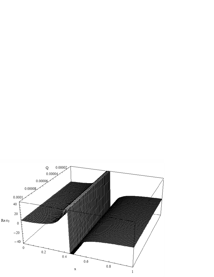
Figure 2: $\mathrm{Re}\pi_{00}(k)$ and the Goldstone mode in the case of $\Psi_{1}$

Let us return to the second case, that of Eq. (II) and dominant intracorrelations. According to Fig. 1, relations Eq. (III) are modified to become:

$$\frac{1}{2\pi}\nabla\times\mathbf{a}^{F\sigma}=2\delta\rho^{F\sigma}+2\delta\rho^{B\sigma},$$

$$\frac{1}{2\pi}\nabla\times\mathbf{a}^{B\sigma}=2\delta\rho^{F\sigma}+\delta\rho^{B\uparrow}+\delta\rho^{B\downarrow}.$$ (40)

It is obvious that in this case we have only $3$ linearly independent gauge fields, namely $a_{C}=\frac{a^{F\uparrow}+a^{F\downarrow}}{2}=\frac{a^{B\uparrow}+a^{B\downarrow}}{2}$, $a_{S}=\frac{a^{F\uparrow}-a^{F\downarrow}}{2}$ and $a_{FS}=\frac{a^{B\uparrow}-a^{B\downarrow}}{2}.$ Introducing the same substitutions as before, the lagrangian again decouples into a charge channel:

$$\mathcal{L}_{C}=K_{00}(\delta a_{0}^{C})^{2}+K_{11}(\delta a_{C})^{2}$$

$$+i\omega\delta\rho_{C}^{B}\theta_{C}-\delta\rho_{C}^{B}\delta a_{0}^{C}-\frac{\overline{\rho}_{b}}{m}k^{2}\theta_{C}^{2}-\frac{\overline{\rho}_{b}}{m}(\delta a_{C})^{2}$$

$$+\frac{ik}{2\pi}a_{0}^{C}a_{C}-\frac{1}{2}V_{C}(\frac{k}{2\pi})^{2}a_{C}^{2},$$ (41)

and a pseudospin channel:

$$\mathcal{L}_{PS}=K_{00}(\delta a_{0}^{S})^{2}+K_{11}(\delta a_{S})^{2}$$

$$+i\omega\delta\rho_{S}^{B}\theta_{S}-\delta\rho_{S}^{B}\delta a_{0}^{FS}-\frac{\overline{\rho}_{b}}{m}k^{2}\theta_{S}^{2}-\frac{\overline{\rho}_{b}}{m}(\delta a_{FS})^{2}$$

$$+\frac{ik}{2\pi}a_{0}^{S}a_{FS}+\frac{ik}{2\pi}a_{0}^{FS}(a_{S}-a_{FS})-\frac{1}{2}V_{S}(\frac{k}{2\pi})^{2}a_{S}^{2},$$ (42)

where $\delta a_{0}^{FS}\equiv a_{0}^{FS}-B_{0},\delta a_{FS}=a_{FS}-B$, all the other symbols have retained their meanings.

This time we will not analyze the charge channel in detail. To this end, we note that the system in incompressible in this sector, the fact which is easily established by integrating out all the gauge fields, densities and boson phase in Eq. (III).

In the pseudospin channel, a calculation of the density-density correlator leads to the conclusion that in this channel the system is compressible (see also Fig. 3). The $\theta-\theta$ correlator is:

$$\langle\theta_{S}(-k)\theta_{S}(k)\rangle=\frac{\frac{1}{k^{2}}\beta\gamma}{(\frac{\omega}{2\pi})^{2}(\beta+\gamma)-\frac{\overline{2\rho}_{b}}{m}\beta\gamma},$$ (43)

where $\beta=\frac{1}{2K_{00}}(\frac{k}{2\pi})^{2}+\frac{2\overline{\rho}_{b}}{m}$, $\gamma=V_{S}(\frac{k}{2\pi})^{2}-2K_{11}.$ For small $k/k_{f}$ and $x$, the correlator diverges for $\omega^{0}=\frac{4\pi\overline{\rho}_{b}}{m}=const$, which obviously contradicts the original assumption for the range of $x$ and hence we reject this pole. For $x\gg 1$ (and still $k\ll k_{f}$), the relations Eq. (III),(III) are approximately $K_{00}\approx-\frac{1}{4\pi x^{2}},K_{11}\approx-\frac{n_{f}}{m}$, and we obtain two poles:

$$\omega^{0}(k)=\frac{4\pi n_{f}}{m}\sqrt{\frac{1}{2}+\eta-\frac{1}{2}\sqrt{1+4\eta}},$$ (44)

$$\Omega^{0}(k)=\frac{4\pi n_{f}}{m}\sqrt{\frac{1}{2}+\eta+\frac{1}{2}\sqrt{1+4\eta}},$$ (45)

where $\eta=\overline{\rho}_{b}/n_{f}$ is the ratio of boson to fermion density (Eqs. (44),(45) hold for any $\eta$, although in the physical limit that we are presently interested in, $\eta$ may be regarded as small). In Fig. 3 we plotted the real part of the density-density correlation function in the case of $\Psi_{2}$, Eq. (57). In contrast to Fig. 2, here we opt for $\omega$ and $Q$ as free parameters and set $d=1.5$ and $\eta=\overline{\rho}_{b}/n_{f}=1/10$ as the more likely values in this case. Distinctive feature of Fig. 3 at $\omega\cong 1$ is the plasma frequency $\Omega^{0}$ and the smaller singularity at $\omega\cong 1/10$ corresponds to $\omega^{0}$. There is also a striking absence of Goldstone mode in this case.

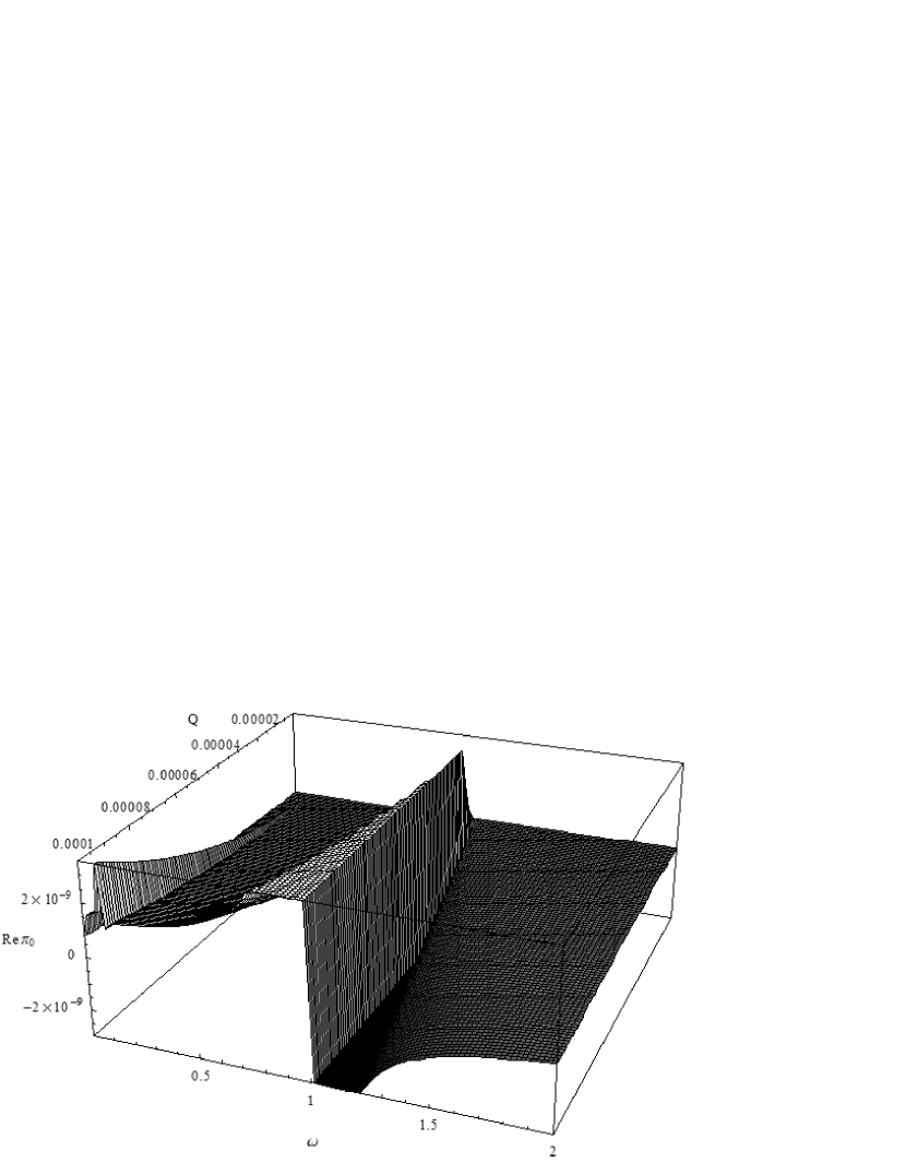
Figure 3: $\mathrm{Re}\pi_{00}(k)$ in the case of $\Psi_{2}$

We now proceed to calculate ODLRO in the pseudospin channel of $\Psi_{2}$. As it turns out, ODLRO will be nontrivially modified and assume algebraic form. We know that interaction does not affect the value of characteristic exponent zhang and therefore set $V_{S}\equiv 0$. Bearing in mind that we work in the long wavelength limit, we arrive at the following expression for the correlator:

$$\langle\theta_{S}(-k)\theta_{S}(k)\rangle=\frac{(2\pi\omega_{P}/k^{2})\left[\omega^{2}-\omega_{P}^{2}\eta\right]}{\left[\omega^{2}-(\omega^{0}(k))^{2}\right]\left[\omega^{2}-(\Omega^{0}(k))^{2}\right]},$$ (46)

where we introduced $\omega_{P}=\frac{4\pi n_{f}}{m}$. After contour integration over $\omega$ zhang :

$$\langle\theta_{S}(-k)\theta_{S}(k)\rangle=-\frac{2\pi}{k^{2}}f(\eta)$$

where $f(\eta)=\frac{1}{\sqrt{1+4\eta}},$ which leads to the algebraic ODLRO:

$$\langle e^{i\theta_{S}(\mathbf{r})}e^{-i\theta_{S}(\mathbf{r^{\prime}})}\rangle\propto\frac{1}{|\mathbf{r}-\mathbf{r^{\prime}}|^{f(\eta)}}$$

$$\approx|\mathbf{r}-\mathbf{r^{\prime}}|^{-(1-2\eta+o(\eta^{2}))}.$$ (47)

This algebraic ODLRO persists as long as $\eta>0$ (function $f$ is positive everywhere in this domain). The expression Eq. (III) is formally reminiscent of BKT XY-ordering, only the role of the temperature is overtaken by the parameter $\eta$ (the analysis of this paper assumes temperature $T=0$). Pursuing this analogy further, we conclude that the relative fluctuations of composite boson and composite fermion density represent the mechanism which may lead to the ultimate breakdown of the $111$-condensate.

IV Evolution of the ground state with $d$

In order to investigate the transition from the incompressible, $111$-like state at lower $d/l_{B}$, to the compressible, possibly vortex metal-like state at higher $d/l_{B}$, we are motivated to introduce what we call generalized vortex metal. In addition to the ordinary vortex metal ($\Psi_{2}$), we include (in each layer) another kind of composite fermions that connect to the composite boson sea as in the case of $\Psi_{1}$. The generalized vortex metal is clearly the only additional option left of connecting electrons divided in composite bosons and composite fermions beside the two extreme cases, $\Psi_{1}$ and $\Psi_{2}$. Again, in this state some of composite fermions connect in the manner of $111$-state to the composite bosons and the rest of composite fermions connect exclusively to the composite bosons of the same layer in the manner of the Rezayi-Read state. This is succinctly represented by the following gauge field constraints:

$$\frac{1}{2\pi}\nabla\times a^{B\sigma}=\delta\rho_{B\uparrow}+\delta\rho_{B\downarrow}+\delta\rho_{F\uparrow}^{(1)}+\delta\rho_{F\downarrow}^{(1)}+2\delta\rho_{F\sigma}^{(2)},$$ (48)

$$\frac{1}{2\pi}\nabla\times a_{1}^{F\sigma}=\delta\rho_{B\uparrow}+\delta\rho_{B\downarrow}+2\delta\rho_{F\sigma}^{(1)}+2\delta\rho_{F\sigma}^{(2)},$$ (49)

$$\frac{1}{2\pi}\nabla\times a_{2}^{F\sigma}=2\delta\rho_{B\sigma}+2\delta\rho_{F\sigma}^{(1)}+2\delta\rho_{F\sigma}^{(2)},$$ (50)

where the superscripts $(1),(2)$ indicate composite fermion species in each layer. Chern-Simons theory easily follows from the above gauge field equations and yields incompressible behavior in the charge channel. In the pseudospin channel:

$$\mathcal{L}_{PS}=K_{00}^{(1)}(\delta a_{0,1}^{FS})^{2}+K_{00}^{(2)}(\delta a_{0,2}^{FS})^{2}$$

$$+K_{11}^{(1)}(\delta a_{1}^{FS})^{2}+K_{11}^{(2)}(\delta a_{2}^{FS})^{2}$$

$$+i\omega\delta\rho_{S}^{B}\theta_{S}-\delta\rho_{S}^{B}\delta a_{0}^{S}-\frac{\overline{\rho}_{b}}{m}k^{2}\theta_{S}^{2}-\frac{\overline{\rho}_{b}}{m}(\delta a_{S})^{2}$$

$$+\frac{ik}{2\pi}a_{0,1}^{FS}(a_{1}^{FS}-a_{S})+\frac{ik}{2\pi}a_{0}^{S}(a_{2}^{FS}-a_{1}^{FS})$$

$$+\frac{ik}{2\pi}a_{0,2}^{FS}a_{S}-\frac{1}{2}V_{S}(\frac{k}{2\pi})^{2}|a_{2}^{FS}|^{2}$$

$$-\frac{1}{2}V_{hc}(\frac{k}{2\pi})^{2}a_{S}(a_{1}^{FS}-a_{S}),$$ (51)

where the linearly independent fields are given by $a_{S}=\frac{a^{B\uparrow}-a^{B\downarrow}}{2}$, $a_{1}^{FS}=\frac{a_{1}^{F\uparrow}-a_{1}^{F\downarrow}}{2}$, $a_{2}^{FS}=\frac{a_{2}^{F\uparrow}-a_{2}^{F\downarrow}}{2}$, subscripts $1,2$ distinguish between composite fermion species and ^S denotes antisymmetric combination of the densities in two layers (like in Sec. III). A noteworthy feature of the lagrangian, Eq. (IV), is the existence of $V_{hc}$, the hard-core repulsion term between the two species of composite fermions inside each layer. The presence of such a term (added by hand) is natural if we imagine composite fermions residing in two separate Fermi spheres. However, the danger of blindly introducing this term is that it may incidentally bring about the incompressible behavior (otherwise not present) in the system. We have verified that this is not the case here i.e. the system remains incompressible whether or not we choose to introduce $V_{hc}$. It therefore appears more intuitive to keep $V_{hc}$, taking the limit $V_{hc}\rightarrow\infty$ in the end. Step by step, eliminating all the gauge fields, we are lead to the following correlation function:

$$\langle\theta_{S}(-k)\theta_{S}(k)\rangle=\frac{V_{S}+\frac{2n_{f2}}{m}(\frac{2\pi}{k})^{2}}{\omega^{2}-(\frac{2\overline{\rho}_{b}V_{S}}{m}k^{2}+(\frac{4\pi}{m})^{2}\overline{\rho}_{b}n_{f2})}$$ (52)

and the low-energy spectrum is dominated by the plasma frequency:

$$\omega^{0}(k)=\frac{4\pi}{m}\sqrt{\overline{\rho}_{b}n_{f2}},$$ (53)

where $n_{f2}$ is the density of the composite fermions which bind exclusively within the layer they belong to. Generalized vortex metal therefore is a state that only supports gapped collective excitations, despite the presence of composite bosons and the kind of composite fermions which enforce interlayer correlation. If it is pertinent to the region of the tunneling experiments of Spielman et al. spielman and counterflow experiments of Kellogg et al. kellogg , we believe that our homogeneous theory of Sec. III,IV then suggests that (generalized) vortex metal can appear only as localized islands (due to presence of disorder at low temperatures) amidst the background of $\Psi_{1}$ phase (Fig. 4). In Fig. 4 depicted are weakly-coupled vortex-antivortex pairs i.e. meron-antimeron pairs (due to the charge degree of freedom, there are four kinds of merons kmoon ) inside the vortex metal phase. They are expected to exist in the vortex-metal phase on the grounds of disordering of the correlated phase. As argued in Ref. milica-preprint, , the inclusion of composite fermions into the $111$ state ($\Psi_{1}$ and $\Psi_{2}$) corresponds to creation of meron-antimeron pairs. There are more pairs and more of larger size as $d$ increases consistent with the BKT picture of the phase that supports algebraic ODLRO, Eq. (III).

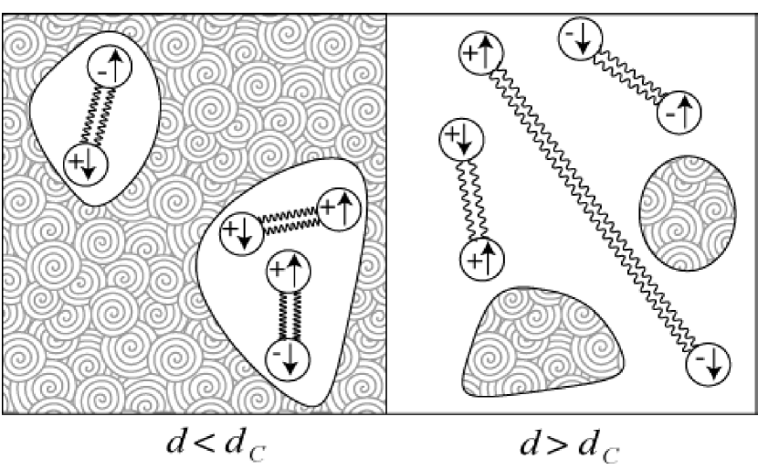
Figure 4: Evolution of the ground state with varying $d$, before and after the transition at $d=d_{C}$. The regions with meron pairs represent the vortex metal ($\Psi_{2}$) phase. The background represents the superfluid ($\Psi_{1}$) phase.

V Further comparison with experiments

In this section we wish to address in depth the potential of the model states, $\Psi_{1}$ and $\Psi_{2}$, in explaining the phenomenology of experiments on bilayer. The key question in this analysis is: what is the nature of the compressible phase corresponding to higher $d/l_{B}$ that still harbors some of the intercorrelation present at lower $d/l_{B}$ kelloggdrag ?

The answer to this question cannot be given by looking at simple transport properties. In Sec. II it was shown that both $\Psi_{1}$ and $\Psi_{2}$ in certain regimes can recover the two main experimental findings of Kellogg et al. in drag experiments: the semicircle law kelloggdrag and the quantization of Hall drag resistance kellogg3 . On the other hand, our Chern-Simons RPA approach at $T=0$ stresses that all that states considered in this paper are incompressible. However, at finite $T$, a finite energy milica-preprint is needed to excite a meron in $\Psi_{2}$ and therefore $\Psi_{2}$ seems like a better candidate for exhibiting compressible behavior at any finite $T$ or, at least, a very small gap. Furthermore, within the vortex metal picture, $\Psi_{2}$ allows the following simple scenario. For $\rho_{bxx}\ll\rho_{fxx}\ll\delta$, one gets the semicircle law derived in Sec. II. As $d/l_{B}$ increases, the density of bosons decreases and one enters the regime $\rho_{fxx}\ll\rho_{bxx}\ll\delta$ where $|\rho_{xx}^{D}|\gg\rho_{xy}^{D}$ (as witnessed in the experiments kelloggdrag ). The persistence of enhanced longitudinal drag resistance kelloggdrag up to very high $d/l_{B}$ provides additional support to our choice of $\Psi_{2}$ which can explain the remaining intercorrelation (drag) in the case where explicit tunneling is absent. Finally, as $\rho_{bxx}\rightarrow\infty$, both resistances go to zero, the bilayer decouples and bosons vanish from the system.

Our picture is certainly incomplete because it does not explicitly include the effects of disorder (which must be very relevant for the physics of bilayer in the regimes $d\sim l_{B}$ - a simple way to see this is to look at the behavior of measured counterflow resistances kellogg ; tutuc $\rho_{xx}^{CF}$, $\rho_{xy}^{CF}$ that enter the insulating regime very quickly after passing through $\nu_{T}=1$). Fertig and Murthy fertig provided a realistic model for the effects of disorder and in their disorder-induced coherence network in the incompressible phase of the bilayer, merons are able to sweep by hopping across the system, causing the activated behavior of resistance (dissipation) in counterflow. This finding is consistent with our own.

At the end our picture is in the spirit of the Stern and Halperin proposal stern-halperin but instead of the $1/2$ compressible phase coexisting in a phase separated picture with the superfluid phase ($\Psi_{1}$), we assume the existence of the vortex metal phase ($\Psi_{2}$). This coincides with the Fertig and Murthy proposal fertig for the incompressible region that explains the ”imperfect” superfluid behavior. It is the continuous extrapolation of this phase separated picture that brings and favors $\Psi_{2}$ for larger $d/l_{B}$ (instead of $\Psi_{1}$). There $\Psi_{2}$ is able to explain the persistence of intercorrelations through enhanced longitudinal drag accompanied by the absence of tunneling and phase coherence. kellogg3

Finally, we are able to account for the effects of the layer density imbalance in tunneling, drag spielman-imbalance and counterflow tutuc-imbalance experiments. Spielman et al. spielman-imbalance observed that small density imbalance stabilizes the resonant tunneling peak - a simple reason for this is that $\Psi_{1}$ can easily accommodate the fluctuations in density (see comment after Eq.(II)). Because of the same reason, Hall drag resistance remains quantized up to larger $d/l_{B}$ in the presence of density imbalance. On the other hand, the enhancement of longitudinal drag resistance at large $d/l_{B}$ was also reported kelloggdrag to be insensitive to density imbalance. While the reason for this cannot be seen only from looking at the form of $\Psi_{2}$ (this state constrains both fermion and boson numbers in two layers, see comment after Eq. II), we believe that meron excitations are responsible for absorbing the density fluctuations, especially at finite $T$.

Recently, the quantum Hall bilayer was probed using resonant Rayleigh scattering rrs for samples with different tunneling amplitudes and when the in-plane magnetic field is present. They detected a nonuniform spatial structure in the vicinity of the transition, suggesting a phase-separated version of the ground state. Our results (for zero tunneling limit and excluding disorder) hint that such phase separation may indeed be necessary to invoke in order to achieve a full description of the strongly-coupled, incompressible phase and the transition in a bilayer.

VI Discussion and Conclusion

In conclusion we showed how two model states, $\Psi_{1}$ and $\Psi_{2}$, can account for the basic phenomenology of the bilayer that came up from various experiments.

A very interesting question pertains the model state $\Psi_{2}$. As effectively a state that represents a collection of meron excitations interacting through topological interactions, a question comes when they are in a confined (dipole) phase and when in a metallic (plasma) phase. So in principle we can expect that the static correlator in Eq. (III) can be reproduced by considering a 2D bosonic model with meron excitations interacting via 2D Coulomb plasma interaction. tsvelik Therefore we believe that the Laughlin ansatz laughlin of considering (static) ground state correlators as statistical models in 2D can be applied here also. We expect that the ground state correlators in a dual approach, in which we switch from composite fermion to meron coordinates, can be mapped to a partition function of a 2D Coulomb plasma. polyakov The 2D Coulomb plasma has two different phases. For large $\beta$ (inverse $T$) the charges form dipoles and the system is with long range correlations (no mass gap). At some critical $\beta$, dissociation of dipoles occurs and we have a plasma phase with a Debye screening, and therefore a mass gap. Thus calculations that will capture more of the meron contribution than our RPA approach in the Chern-Simons theory may find a transition and exponential decay of the correlator (Eq. (III)), before reaching $\overline{\rho}_{b}=0$ limit. Indeed our ODLRO exponent in Eq. (III) at $\overline{\rho}_{b}=0$ is $1$ which is well above the exponent of the BKT transition or critical exponent $1/4$. At that point our system may develop a gap in the pseudospin channel and completely lose interlayer coherence (exponential decay of correlators). Furthermore, we expect that the superfluid portion of the composite boson density will disappear leading to compressible behavior in the charge channel. zhang This is all consistent with experiments kellogg3 ; kelloggdrag which find that, at $d/l_{B}\approx 1.84$, the vanishing of the conventional quantum Hall effect and the system’s Josephson-like tunneling characteristics occurs simultaneously. Intercorrelated bosons continue to exist without a superfluid property and lead to enhanced $\nu=1$ drag at large $d/l_{B}$. They disappear from the system around $d/l_{B}\approx 2.6$ kelloggdrag .

VII Acknowledgment

The work was supported by Grant No. 141035 of the Ministry of Science of the Republic of Serbia.

Appendix A

In order to extract the response functions in functional integral formalism, one needs to integrate over all degrees of freedom except those of the external fields. The integration of these fields in the RPA approximation proverbially reduces to the Gaussian integral:

$$\int d(z,z*)\verb"exp"\left[-z*wz+u*z+vz*\right]$$

$$=\frac{\pi}{w}\verb"exp"\left[\frac{u*v}{w}\right],\mathrm{Re}w>0.$$

For the pseudospin channel in the case of $\Psi_{1}$ (Eq. (II)) we therefore obtain the following linear response:

$$\pi_{00}(k)=\frac{1}{\Xi}(\Omega(3V_{S}+2\alpha)+1),$$ (54)

$$\pi_{01}(k)=\pi_{10}(k)=\frac{1}{\Xi}\frac{-i\pi}{k}K_{11}(1+\Omega V_{S}),$$ (55)

$$\pi_{11}(k)=\frac{1}{\Xi}\{2V_{S}(1-\Omega V_{S})(K_{11}-\frac{\overline{\rho}_{b}}{m})$$

$$+K_{11}/K_{00}-4\alpha\frac{\overline{\rho}_{b}}{m}\},$$ (56)

where $\alpha\equiv\frac{1}{4}K_{00}^{-1}-K_{11}(\frac{2\pi}{k})^{2},$ $\Omega\equiv\left[V_{S}-\frac{m\omega^{2}}{2\overline{\rho}_{b}k^{2}}\right]^{-1}$ and $\Xi=V_{S}(1-\Omega V_{S})+2\alpha$.

The response functions in the case of the pseudospin channel of $\Psi_{2}$ (Eq. (II)) are:

$$\pi_{00}=\frac{1}{\Delta}(\frac{k}{2\pi})^{2},$$ (57)

$$\pi_{01}=\pi_{10}=\frac{1}{\Delta}\frac{ik}{2\pi}\Lambda,$$ (58)

$$\pi_{11}=\frac{1}{\Delta}\{\Lambda^{2}+\Delta(2K_{11}-\frac{2\overline{\rho}_{b}}{m}-16W^{4}(\frac{2\pi\overline{\rho}_{b}}{m\omega})^{4})\},$$ (59)

where $W^{4}\equiv-\frac{(\frac{m\omega^{2}}{2\overline{\rho}_{b}(2\pi)^{2}})^{2}}{\frac{1}{2K_{00}}(\frac{k}{2\pi})^{2}-\frac{m\omega^{2}}{2\overline{\rho}_{b}(2\pi)^{2}}+\frac{2\overline{\rho}_{b}}{m}},$ $\Delta\equiv W^{4}-\frac{m\omega^{2}}{2\overline{\rho}_{b}(2\pi)^{2}}-2K_{11}+V_{S}(\frac{k}{2\pi})^{2},$ $\Lambda\equiv 4W^{4}(\frac{2\pi\overline{\rho}_{b}}{m\omega})^{2}-2K_{11}.$

References

- (1) B.I. Halperin, Helv. Phys. Acta 56, 75 (1983).
- (2) K. Moon, H. Mori, K. Yang, S.M. Girvin, A.H. MacDonald, L. Zheng, D. Yoshioka, and S.-C. Zhang, Phys. Rev. B 51, 5138 (1995).
- (3) H.A. Fertig, Phys. Rev. B 40, 1087 (1989).
- (4) I. Stanić and M.V. Milovanović, Phys. Rev. B 71, 035329 (2005).
- (5) I.B. Spielman, J.P. Eisenstein, L.N. Pfeiffer, and K.W. West, Phys. Rev. Lett. 84, 5808 (2000); ibid 87, 036803 (2001).
- (6) M. Kellogg, J.P. Eisenstein, L.N. Pfeiffer, and K.W. West, Phys. Rev. Lett. 93, 036801 (2004).
- (7) E. Tutuc, M. Shayegan, and D.A. Huse, Phys. Rev. Lett. 93, 036802 (2004).
- (8) S.H. Simon, E.H. Rezayi, and M.V. Milovanović, Phys. Rev. Lett. 91, 046803 (2003).
- (9) M. Kellogg, J.P. Eisenstein, L.N. Pfeiffer, and K.W. West, Phys. Rev. Lett. 90, 246801 (2003).
- (10) M.V. Milovanović, Phys. Rev. B 75, 035314 (2007).
- (11) R.B. Laughlin, Phys. Rev. Lett. 50, 1395 (1983).
- (12) E.H. Rezayi and N. Read, Phys. Rev. Lett. 72, 900 (1994).
- (13) A. Stern and B.I. Halperin, Phys. Rev. Lett. 88, 106801 (2002).
- (14) R.L. Willett, Adv. Phys. 46, 447 (1997).
- (15) S.C. Zhang, T. H. Hansson, and S. Kivelson, Phys. Rev. Lett. 62, 980 (1989).
- (16) B.I. Halperin, P.A. Lee, and N. Read, Phys. Rev. B 47, 7312 (1993).
- (17) G. Murthy and R. Shankar, Rev. Mod. Phys. 75, 1101 (2003).
- (18) B. Blok and X.-G. Wen, Phys. Rev. B 42, 8145 (1990); ibid. 43, 8337 (1991).
- (19) S.-C. Zhang, Int. J. of Mod. Phys. B 6, 25 (1992).
- (20) M. Kellogg, J.B. Spielman, J.P. Eisenstein, L.N. Pfeiffer, and K.W. West, Phys. Rev. Lett. 88, 126804 (2002).
- (21) H.A. Fertig and G. Murthy, Phys. Rev. Lett. 95, 156802 (2005).
- (22) I.B. Spielman, M. Kellogg, J.P. Eisenstein, L.N. Pfeiffer and K.W. West, Phys. Rev. B 70, 081303(R), 2004.
- (23) E. Tutuc and M. Shayegan, Phys. Rev. B 72, 081307(R), (2005).
- (24) S. Luin, V. Pellegrini, A. Pinczuk, B.S. Dennis, L.N. Pfeiffer and K.W. West, Phys. Rev. Lett. 97, 216802 (2006).
- (25) A.O. Gogolin, A.A. Nersesyan, and A.M. Tsvelik, Bosonization and Strongly Correlated Systems (Cambridge University Press, Cambridge, 1998)
- (26) R.B. Laughlin in The Quantum Hall Effect, 2nd. ed., edited by R.E. Prange and S.M. Girvin (Springer, New York, 1990).
- (27) A.M. Polyakov, Gauge Fields and Strings (Harwood Academic Publishers, Chur, 1989)