Transverse transport of solutes between co-flowing pressure-driven streams for microfluidic studies of diffusion/reaction processes

Abstract

We consider a situation commonly encountered in microfluidics: two streams of miscible liquids are brought at a junction to flow side by side within a microchannel, allowing solutes to diffuse from one stream to the other and possibly react. We focus on two model problems: (i) the transverse transport of a single solute from a stream into the adjacent one, (ii) the transport of the product of a diffusion-controlled chemical reaction between solutes originating from the two streams. Our description is made general through a non-dimensionalized formulation that incorporates both the parabolic Poiseuille velocity profile along the channel and thermal diffusion in the transverse direction. Numerical analysis over a wide range of the streamwise coordinate $x$ reveal different regimes. Close to the top and the bottom walls of the microchannel, the extent of the diffusive zone follows three distinct power law regimes as $x$ is increased, characterized respectively by the exponents $1/2$, $1/3$ and $1/2$. Simple analytical arguments are proposed to account for these results.

I Introduction

Microfluidics is a very promising format to measure the dynamics of different processes: diffusion of a solute Kamholz et al. (2001); Culbertson et al. (2002); Salmon et al. (2005a), protein folding Knight et al. (1998); Pollack et al. (2001); Pan et al. (2002), kinetics of chemical reactions Pabit and Hagen (2002); Salmon et al. (2005b)…  (see Refs. Stone et al. (2004); Squires and Quake (2005); Vilkner et al. (2004) for reviews on microfluidics). In some of these approaches, one follows the reaction-diffusion dynamics of solutes between parallel streams. Figure 1 displays the simplest case of a Y-junction commonly encountered in microfluidic experiments, where two liquids are injected in a main microchannel.

Figure 1: Geometry of the problem. The origin of the axes is set at the junction between the two inlets and $Z$ ranges between $\pm d/2$. A and B indicates the two arms in which the miscible liquids are injected. The liquids may react when they interdiffuse into each other.

Since flows are laminar given the small length scales and velocities involved, the liquids only mix by transverse diffusion, and one can relate the distance downstream the channel, to the time elapsed since the two streams where put into contact. Essentially, if the average velocity in the channel is $V$, one expects that the situation at a distance $X$ from the junction corresponds to the outcome of diffusion-reaction over a time $t=X/V$, so that for example, simple interdiffusion leads to a diffusion zone of width $Y\sim(2DX/V)^{1/2}$.

However, in confined geometries the situation is actually more complex as pressure-driven flows are heterogenous (parabolic velocity profile), resulting in residence times that vary with the distance to the walls. Therefore, in order to extract from these experiments physical parameters such as diffusion coefficients or rate constants, it is essential to understand correctly the mass transport phenomena in microchannels.

In this context, Ismagilov et al. Ismagilov et al. (2000) have studied using confocal microscopy, the formation and the diffusion of a fluorescent product in the diffusion cone of two reactive miscible solutions flowing side by side in a microchannel (the geometry is the same as displayed in Fig. 1). They have shown, both theoretically and experimentally, that the extent of the transverse diffusive zone near the top and the bottom walls ($Z=\pm d/2$) scales as $Y\sim X^{1/3}$, i.e. follows a $1/3$ power law in the streamwise coordinate $X$. In the central plane of the microchannel, they observed the classical $1/2$ power law for diffusive processes $Y\sim X^{1/2}$. Such behaviours are due to the coupling of transverse diffusion and velocity gradients in the channel. These measured exponents can be accounted for by arguments derived from the classical L v que problem Stone (1989). Kamholz et al. have performed numerical simulations of the same problem Kamholz and Yager (2002), and found the different regimes expected. However, their results concern only specific sets of dimensionalized parameters which makes it difficult to apply them to other experimental configurations. In addition, some of the results displayed in Ref. Kamholz and Yager (2002) are inconsistent with findings shown later in the present manuscript. More recently, a significant improvement has been brought by Jim nez who performed numerical simulations of the same problem using dimensionless equationsJiménez (2005). His work accounts for the different regimes observed experimentally, and the author also clarifies these results using analytical solutions of the concentration profile in the range of small and large $X$. In a recent paper (Supporting Information of Ref. Salmon et al. (2005b)), we have studied the effect of the Poiseuille flow developped in a microchannel of high aspect ratio, on the reaction-diffusion dynamics occurring in the diffusion cone of two reactive solutions injected side by side. Through numerical simulations, we showed that for the high aspect ratio studied, a 2D description in terms of height-averaged concentrations and velocities was appropriate and could be safely used to extract the rate constant of the reaction from experimental data.

Our aim in this paper is to revisit formally these transverse transport problems so as to provide generally applicable insights as to the outcome of experiments performed in arbitrary conditions (flow rate, geometry,…), but for the requirement that the Péclet number be large (see below). In the first part of this paper, we discuss the simple case of the transverse diffusion of a solute, using numerics and simple analytical arguments in a generic non-dimensionalized formulation. We clarify that the $1/3$ power law behaviour for transverse spreading ($Y\sim X^{1/3}$) holds after the junction in layers close to the walls, the thickness of which increases as $\sim X^{1/3}$. For a small but finite distance from the walls (i.e. for a given $Z$), the transverse extent $Y$ of the diffusion zone actually follows successively three power law regimes in $X$ as $X$ is increased, with exponents $1/2$, then $1/3$ and finally $1/2$ again. We then discuss the relevance of these findings for published data. In a second part, we study the more complex case of coupled diffusion and reaction of two reactive solutes yielding the apparition and diffusion of a product in the neighbourhood of the interface between the two streams. Most of the phenomenology described in the first part is shown to persist when the kinetics of the reaction is fast compared to diffusion, with however a few qualitative differences that are pointed out.

II Diffusion of a solute into a neighbour stream

II.1 Assumptions of the model

We consider a microchannel with a high aspect ratio $\Gamma=L/d\gg 1$, as depicted in Fig. 1. Two solutions of the same solvent are injected at a same constant flow rate in the two arms of the microchannel: (i) the solution flown through arm A contains at a dilute level a solute A, whereas (ii) pure solvent is flown through the other arm B. We are interested in the concentration profiles $A(X,Y,Z)$ of this solute downstream. Given our microfluidic motivation, we consider that the flow is strictly laminar (small Reynolds number) and that the solute only disperses by molecular diffusion. We also suppose that the diffusion coefficient $D$ of the solute, as well as the fluid viscosity and density, are constant for the dilute solutions considered here.

With these assumptions, the velocity profile is locally parabolic and well described by Hele-Shaw formulas (except for positions $Y$ at a distance $d$ or smaller from the two lateral walls at $Y=\pm L/2$). Typically after an entrance region of order $L$ from the junction, the flow takes the simple form ${\bf v}(X,Y,Z)=v(Z){\bf X}$ with

$$v(Z)=U\left(1-\left(\frac{Z}{d/2}\right)^{2}\right)\,,$$ (1)

with $U$ the maximal velocity.

We now write the equation describing the transport of the solute resulting from convection in this velocity field and thermal diffusion. We focus immediately on the limit of high Péclet numbers, i.e. $\text{Pe}=Ud/D\gg 1$, where one can neglect the diffusion along the flow direction, and the concentration $A$ of solute A evolves according to

$$v(Z)\partial_{X}A(X,Y,Z)=D(\partial_{Y}^{2}+\partial_{Z}^{2})A(X,Y,Z)\,.$$ (2)

If we neglect entrance effects, i.e. if we assume that the solute does not significantly diffuse transversely in the entrance zone, the concentration downstream can be found by solving Eq. (2) with no-flux boundary conditions on the lateral walls, and "initial" conditions at $X\simeq 0$: $A(Y,Z)=0$ for $Y>0$ and $A(Y,Z)=A_{0}$ for $Y<0$.

We make the problem non-dimensional using

$$x=X/(d\,\text{Pe}),\,\,z=Z/d,\,\,y=Y/d,\,\,\text{and}\,\,a=A/A_{0},$$ (3)

so that Eq. (2) takes a parameter-free form

$$(1-(2z)^{2})\,\partial_{x}a(x,y,z)=(\partial_{y}^{2}+\partial_{z}^{2})a(x,y,z)\,.$$ (4)

II.2 Numerical computation of the model

We solve Eq. (4) using a simple numerical approach (the Euler method). We descretize the $(y,z)$ plane using a 2D "grid" with nodes $y_{j}=-\Gamma/2+\text{d}y/2+(j-1)\text{d}y$, and $z_{j}=-1/2+\text{d}z/2+(j-1)\text{d}z$, with $\text{d}y=\Gamma/n$ and $\text{d}z=1/p$, with typically $p=60$ points across the channel height and $n=80$ points across the channel width. We impose the classical no-flux boundary conditions at the walls at $z=\pm 1/2$ and $y=\pm\Gamma/2$. As in Ref. Jiménez (2005), we perform different simulations and overlap their outcome to cover a wide range of values of $x$. More precisely, to reach sufficient accuracy over this whole range, the resolution on the $y$-axis is varied through variations of $\Gamma$, each simulations being terminated before the solute diffuses up to the side walls as $y=\pm\Gamma/2$.

II.3 Numerical results

Typical concentration profiles within cross-sections at different downstream locations $x$ are shown in Fig. 2.

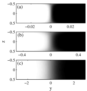
Figure 2: Typical $z$-$y$ slices of the concentration $a$ of the solute at (a) $x=10^{-6}$, (b) $10^{-3}$, and (c) $10^{-1}$. A linear gray scale is used to code the values of $a$: black corresponds to 0, and white corresponds to 1.

For $x\lesssim 0.1$, the concentration profiles are not homogenized across the height of the microchannel, as already explained in Refs. Ismagilov et al. (2000); Kamholz and Yager (2002); Jiménez (2005). This is a consequence of the dispersion of the residence times in the microchannel due to the Poiseuille flow. For $x\gtrsim 0.1$, one almost recovers homogeneous profiles. This is expected since the criterion for the solute to sample all $z$-positions by diffusion reads roughly $x\gtrsim 1/8$, as the solute has to diffuse over the half height of the channel so that $2DX/V\gtrsim(d/2)^{2}$.

To get further insight into the broadening with $x$ of the concentration front, we define an average width $w(x,z)$ of the concentration profiles, at height $z$ and distance $x$, as

$$2w^{2}(x,z)=\int_{-\Gamma/2}^{\Gamma/2}\text{d}y\,y^{2}\partial_{y}a(x,y,z)/\int_{-\Gamma/2}^{\Gamma/2}\text{d}y\,\partial_{y}a(x,y,z)\,.$$ (5)

In the ideal case of simple diffusion with a homogeneous velocity profile (plug flow), $a(x,y,z)=0.5\left(1+\text{erf}(-y/(2w(x))\right)$, and the diffuse broadening obeys the simple diffusive scaling $w(x)\sim x^{1/2}$ with an exponent $1/2$.

The curves $w(x,z)$ vs. $x$ for a Poiseuille flow profile are shown in Fig. 3 for several heights $z$ in the microchannel.

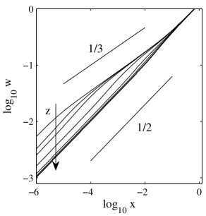
Figure 3: $\log_{10}(w)$ vs. $\log_{10}(x)$ for different $z$. The arrow indicates the range of increasing $z$ from $-1/2+\text{d}z/2$ to $-\text{d}z/2$ ($\text{d}z=1/60$ in the present simulations). The two continous lines indicate the $1/2$ and $1/3$ power law behaviours.

For values of $x$ below 0.1, a dispersion of the widths $w(x,z)$ is visible, as expected from Fig. 2: the concentration profiles are wider close to the bottom and the top walls. For values of $x$ greater than 0.1, all the curves collapse and a homogenous (along $z$) diffusion along $y$ is recovered.

To describe in more detail the local behaviour of $w(x,z)$ vs. $x$, we fit these curves locally by power laws $w(x,z)\sim x^{\alpha(x,z)}$ over a sliding decade of $x$, from $x\approx 10^{-6}$ to $x\approx 1$. The exponents $\alpha(x,z)$ found by such an analysis are displayed in Fig. 4.

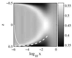
Figure 4: $\alpha(z,x)$ vs. $\log_{10}(x)$ and $z$. The exponents $\alpha(x,z)$ are estimated by local fits of the curves displayed in Fig. 3 by power laws. The dashed white line indicates $u=1$ [see Eqs. (6)–(10)], and the continous white line corresponds to Eq. (21) with $\text{Pe}=1000$. For clarity, these two lines have been only plotted for $z>0$.

For very low values of $x<10^{-5}$, one observes that $w(x,z)\sim x^{1/2}$ for all the investigated range of $z$. For $10^{-5}<x<10^{-1}$, the curves corresponding to $z$-positions close to the walls reach a $1/3$ power law regime. In this regime, the local exponent in the middle of the microchannel deviates from $1/2$, reaching values up to $0.55$. Eventually, the classical $1/2$ exponent of homogenous diffusion is recovered for $x\gtrsim 0.1$.

At small but finite distance from the walls ($\lesssim 0.2$), we therefore predict a succession of three power law regimes with exponents $1/2$, $1/3$, and $1/2$. The transition from the $1/2$ to the $1/3$ regime occurs earlier for values of $z$ closer to the walls. To our knowledge, no experiments have shown this transition.

In many experiments, the quantity measured is the concentration field averaged over the thickness of the microchannel. We compute this quantity from our solutions of Eq. (4), and define the corresponding width $w_{m}(x)$ describing broadening in this averaged map using the analog of Eq. (5). We can now quantitatively answer one of the main points raised in the introduction: for very thin channel, how good/bad is the approximation consisting in assuming fast diffusion over $Z$ so that flow heterogeneities can altogether be neglected ? This approximation leads to the homogeneous diffusion prediction $w(x)=\sqrt{3x/2}$. We compare it to the real width of the averaged map $w_{m}(x)$ by plotting in Fig. 5(a) a measure of the relative error made in using this approximation $\delta(x)=w_{m}(x)/\sqrt{3x/2}-1$.

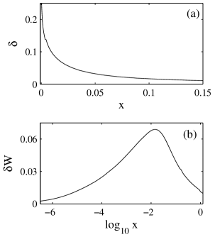
Figure 5: (a) $\delta=w_{m}(x)/\sqrt{3x/2}-1$ vs. $x$. $\delta$ allows one to estimate the deviation between the width of the averaged concentration profiles and the solution when the Poiseuille flow has not been taken into account. (b) $\delta W$ vs. $x$. $\delta W$ is the difference between the widths of the diffusion zone at $z\rightarrow\pm 1/2$ and at $z=0$.

From the plot it is clear that while important deviations are observed at very short distances, the error is less than 5% for all values of $x$ larger than $0.03$, which corresponds in real units to distances after the junction $X\leq 0.03\,\text{Pe}\,d$.

Figure 5(b) shows another measure of the heterogeneity along $z$ of the concentration profile: $\delta W$, the difference between the widths of the interdiffusion zone at the wall and at $z=0$. As can be seen on this plot, the maximal difference is reached for $x\approx 10^{-2}$, and corresponds to values of about 7% (in real units $0.07\,d$).

II.4 Transition of the exponent from 1/2 to 1/3 close to the walls

We present now analytical arguments that help understand the above results, namely the transition from the $1/2$ to the $1/3$ regime observed close to the walls, for a value of $x$ that increases with the distance to the wall.

We focus on the vicinity of the bottom wall, and make therefore the additional reasonable approximation that the velocity profile there is almost linear, so: $v(Z^{\prime})=\dot{\gamma}Z^{\prime}$, where $\dot{\gamma}=4U/d$ is the local shear rate at the wall and $Z^{\prime}=Z+d/2$ is the distance to the wall. In the diffusion process, the only relevant length scale is therefore $l=\sqrt{D/\dot{\gamma}}$. Close to the wall, the concentration field of the solute A evolves through

$$Z^{\prime}\partial_{X}a=l^{2}(\partial_{Y}^{2}+\partial_{Z^{\prime}}^{2})a\,.$$ (6)

We make a change of variables akin to the classical treatment of the Lév que problem:

$$u =Z^{\prime}/(X^{1/3}l^{2/3})\,,$$ (7)

$$v =Y/(X^{1/3}l^{2/3})\,,$$ (8)

$$a =F(u,v)\,,$$ (9)

so that Eq. (6) reads

$$(\partial_{u}^{2}+\partial_{v}^{2})F=-\frac{1}{3}u[u\partial_{u}F+v\partial_{v}F]\,.$$ (10)

The boundary and initial conditions

$$(\partial_{Z^{\prime}}a)_{Z^{\prime}=0}=0\,,$$ (11)

$$a=0~{}~{}\text{for}~{}~{}Y>0,~{}~{}\text{and}~{}~{}a=1~{}~{}\text{for}~{}~{}Y<0\,,$$ (12)

read now

$$(\partial_{u}F)_{u=0}=0\,,$$ (13)

$$\lim_{v\rightarrow+\infty}F=1\,,$$ (14)

$$\lim_{v\rightarrow-\infty}F=0\,.$$ (15)

Using Eq. (5), the local width of the concentration profile is:

$$w^{2}(X,Z^{\prime})=X^{2/3}l^{4/3}G(u)\,,$$ (16)

where

$$G(u)=\int\text{d}v\,v^{2}\partial_{v}F\,.$$ (17)

Using Eq. (10), $G(u)$ has to satisfy

$$G^{\prime\prime}+\frac{u^{2}}{3}G^{\prime}-\frac{2u}{3}G+2=0\,,$$ (18)

with

$$(\partial_{u}G)_{u=0}=0\,,$$ (19)

$$\lim_{u\rightarrow\infty}G=0\,.$$ (20)

Close to the wall $Z^{\prime}\sim 0$ and $u\sim 0$, the conditions $(\partial_{u}G)_{u=0}=0$ therefore gives $G(u)=\text{cste}$ and $w(X,Z)\sim X^{1/3}Z^{\prime 2/3}$. This is the classical results of the L v que problem Stone (1989) and shown by our simulations for positions $Z^{\prime}$ very close to the walls, for $x<0.1$. For large $u$, one should have $w^{2}(X,Z^{\prime})=KDX/(\dot{\gamma}Z^{\prime})$, and therefore $G(u)=K/u$. Using Eq. (18), one has $K=2$ which is the classical diffusive behaviour.

Figure 6 helps to sum up these results.

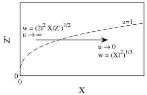
Figure 6: Schematic representation of the asymptotic behaviour of the solutions of Eq. (18). The line $X=0$ corresponds to $u\sim\infty$ for finite $Z^{\prime}$. The dashed line indicates $u=1$.

At a given position $Z^{\prime}$, one encounters two regimes as $X$ is increased. For $X\sim 0$, one has $u\rightarrow\infty$ and $w(X,Z^{\prime})\sim X^{1/2}$, and for large $X$ one has $u\rightarrow 0$ and $w(X,Z^{\prime})\sim X^{1/3}$. The boundary between these two regimes can be estimated using the curve $u=1$, i.e. $Z^{\prime}=X^{1/3}l^{2/3}$. In the previous systems of units [see Eq. (3)], $u=1$ reads $z=\pm 0.5\mp(x/4)^{1/3}$. One of these two boundaries is shown in Fig. 4 and a good agreement is observed with the frontier between the $1/2$ and $1/3$ regimes.

Note that this simple argument, that permits to apprehend the transition from 1/2 to 1/3, is strictly speaking limited to the vicinity of the walls. Further away, one should take into account the curvature of the flow profile, and eventually describe the merger of the two zones of $1/3$ behaviour.

II.5 Validity of the approximations embedded in the model

We have altogether neglected longitudinal diffusion (along $X$) on the ground of a large Péclet number $\text{Pe}=Ud/D\gg 1$. To assess more locally the range of validity of this approximation, a useful quantity is $v(Z)X/D$, the Péclet number using the length scale $X$ and the velocity $v(Z)$. Indeed, positions $X,Z$ such that $v(Z)X/D\gg 1$ correspond to the region where diffusion along the axial direction is negligible. The curve $v(Z)X/D=1$ is thus a reasonable estimate for the boundary of the domain where our approximation should be valid. In non-dimensionalized units, this boundary reads

$$x=\frac{1}{\text{Pe}^{2}}\frac{1}{1-(2z)^{2}}\,,$$ (21)

and is plotted in Fig. 4 for the case $\text{Pe}=1000$. It intersects the curve $u=1$ indicating the growing boundary layer corresponding to the $1/3$ power law regime for values $x\approx 1/\text{Pe}^{2}$ and $z\pm 1/2\approx\pm(1/4\text{Pe}^{2})^{1/3}$. So, to visualize experimentally comfortably this 1/3 regime, one should use high Péclet numbers, and focus on positions $(z,x)$ given by the previous relations. For $\text{Pe}=1000$, the crossing point (see Fig. 4) is at $z\pm 1/2\approx 6\,10^{-3}$, i.e. below 1% of the height of the microchannel, leaving ample space for observing this regime.

Another issue concerns having neglected any specific effect in the entrance region of size $L$. In this zone, the velocity profile evolves from what it was in each branch into its final form given Eq. (1). The extent of this region in non-dimensional units is of the order of $x\lesssim(L/d)\,\text{Pe}^{-1}$, so that unless Pe is really very large, this region will overlap with the $1/3$-regime. For example for $\text{Pe}=1000$ and $L/d=10$, the entrance region corresponds to $x\lesssim 0.01$. However, we do not think that a refined description with a model for this entrance region would modify the picture presented. Indeed, it takes only a distance of order $X\sim d$ after the apex of the junction to reach a parabolic profile in the interfacial region, and it is only the amplitude of this parabola (the local maximal velocity) that relaxes to its asymptotic value over $X\sim L$.

II.6 Comparison with experiments

We now compare our results with existing experimental data. Kamholz et al. have measured the diffusivity of various fluorescent molecules using the device sketched in Fig. 1 Kamholz et al. (2001). They used microchannels of small thickness ($d=10~{}\mu$m) and models assuming fast averaging over this thin dimension to extract the diffusion constants. Our analysis shows that this procedure was actually appropriate given its simplicity. Indeed, their "worst" experimental configuration (highest flow rate $\approx 1000~{}$nL/s, and smallest diffusivity $D=6.2\,10^{-11}~{}$m²/s for streptavidin, so $\text{Pe}\approx 8000$), corresponds to measurements taken at $x\approx 0.05$ in non-dimensionalized units, for which the relative error from using the simplified model is less than 5% as can be seen on Fig. 5(a) (even if the difference of width $\delta W$ is maximal at this position [see Fig. 5(b)]).

As pointed in the introduction of the present paper, our results are not consistent with the theoretical data discussed in Ref. Kamholz and Yager (2002). In this work, the authors do no use non-dimensionalized equations but have computed the concentration profiles for a specific case (flow rate $Q=42~{}$nL/s, $L=2405~{}\mu$m, $d=10~{}\mu$m, $D=3.4~{}10^{-10}~{}$m² s^-1, leading to $\text{Pe}\approx 50$). They found, in the midplane of the channel ($z=0$) and in the range $x=10^{-2}$–$10^{-1}$, a power law regime for the transverse spreading given by an exponent 2/3. Such a result is not consistent with the data displayed in Fig. 4, and we believe it is due to the fitting procedure of the curves $w(x,z)$ vs. $x$. More important, the authors claim that a model with a homogeneous velocity profile (1D model) overpredicts the diffusion width by $\approx 35\%$, even for distances $X=1000~{}\mu$m, i.e. $x=2$ in non-dimensionalized units. Such results are in contradiction with our data [see Fig. 5(a)].

We now consider the data of Ismagilov et al. Ismagilov et al. (2000), who used confocal fluorescence microscopy to measure the transverse diffusive broadening of a fluorescent probe formed as the product of a reaction involving diffusing reactants originating from solutions flowing side by side in a microchannel. Clearly, that situation is more complex than the one analyzed above as both diffusion and reaction come into play. The data displayed in Ref. Ismagilov et al. (2000), more precisely in their Fig. 2, concern a microchannel of thickness $d=105~{}\mu$m, a maximal velocity of the order of $12$ cm/s, and an investigated range of $X$ ranging between $10^{2}$ and $10^{4}~{}\mu$m. Taking $D\approx 10^{-9}$ m²/s to estimate $\text{Pe}\approx 12600$, the dimensionless $x$ ranges roughly between $10^{-4}$ and $10^{-2}$. As can be seen on Figs. 3 and 4, our analysis suggests that in this range, the boundary layers where the transverse diffusive zone widens as $x^{1/3}$ should occupy a significant portion of the microchannel, in agreement with the observation by the authors of such a scaling for the broadening close to the walls. However, as can be seen on Fig. 5(b), from our analysis, the difference between diffusive width at the walls and at the center should be less than $\approx 0.07d$, i.e. $\approx 7~{}\mu$m. The values reported in Ref. Ismagilov et al. (2000) lead to a somewhat larger estimate ($\approx 30~{}\mu$m)– the difference is too large to be simply the result of a slightly different definition of the diffusion width $w$ [see Eq. (5)]–. Furthermore, the interdiffusion zones they observed have a different shape than those displayed in Fig. 2. We conclude that while the presence and location of a "1/3 regime" is robust to the differences between the two situations, some features do show a difference. To confirm this we now proceed to a brief investigation of a reaction-diffusion model.

III Diffusion of quickly reacting species

III.1 Assumptions of the model

We turn to the case of a chemical reaction $\text{A}+\text{B}\rightleftarrows{\text{C}}$. Different groups have theoretically investigated the solutions of the unidimensional problem of reaction-diffusion without advection Gálfi and Rácz (1988); Taitelbaum et al. (1992); Bazant and Stone (2000). These works mainly deal with irreversible reactions $\text{A}+\text{B}\rightarrow{\text{C}}$, and have provided scaling laws of the width of the reaction front, both in the asymptotic and in the short-time limits. In our case, we are interested in the concentration map of the product C, when the two reactants, A and B, are injected in the two arms of the microchannel (see Fig. 1), at a same given constant flow rate, and at concentrations $a_{0}$ and $b_{0}$ respectively. As above, we restrict ourselves to dilute solutions, and further focus on fast chemical reactions, so that chemical equilibrium $AB/C=K_{eq}$ is satisfied at each point of the microchannel ($K_{eq}$ is the equilibrium constant of the reaction, and $A$, $B$ and $C$ are the concentrations of species A, B, and C respectively). To reduce the number of independent parameters, we take the diffusion coefficients of species B and C to be almost identical, i.e. $D_{C}\approx D_{B}$. This should well describe complexation reactions where A is a small molecule that can not affect the diffusion coefficient of the larger B. Reaction-diffusion dynamics in a microchannel with the same assumptions than previously read

$$v(Z)\partial_{X}A =-R+D_{A}(\partial_{Y}^{2}+\partial_{Z}^{2})A\,,$$ (22)

$$v(Z)\partial_{X}B =-R+D_{B}(\partial_{Y}^{2}+\partial_{Z}^{2})B\,,$$

$$v(Z)\partial_{X}C =+R+D_{B}(\partial_{Y}^{2}+\partial_{Z}^{2})C\,,$$

$R$ corresponds to the reaction term. Since the reaction is very fast, $AB/C=K_{eq}$, and the problem is governed by only two equations. Considering species conservation, we focus on the combination: $P=A+C$, and $Q=B+C$, so Eqs. (22) read

$$v(Z)\partial_{X}P = D_{A}(\partial_{Y}^{2}+\partial_{Z}^{2})P$$

$$+ (D_{A}-D_{B})(\partial_{Y}^{2}+\partial_{Z}^{2})C\,,$$

$$v(Z)\partial_{X}Q = D_{B}(\partial_{Y}^{2}+\partial_{Z}^{2})Q\,,$$

where $C=C(P,Q)$ is to be understood as the implicit solution the local chemical equilibrium:

$$K_{eq}C=(P-C)(Q-C)\,.$$ (24)

We move to dimensionless variables,

$$p=P/a_{0}\,,~{}~{}~{}~{}~{}q=Q/b_{0}\,,~{}~{}~{}~{}c=C/(a_{0}b_{0})^{1/2}\,,$$ (25)

and again :

$$x=X/(d\,\text{Pe}),\,\,\,\,\,z=Z/d,\,\,\,\,\text{and}\,\,\,\,y=Y/d\,,$$ (26)

with $\text{Pe}=Ud/D_{A}$, Eqs. (III.1) and (24) read

$$(1-(2z)^{2})\,\partial_{x}p=(\partial_{y}^{2}+\partial_{z}^{2})(p+\frac{\chi^{2}-1}{\beta}c)\,,$$ (27)

$$(1-(2z)^{2})\,\partial_{x}q=\chi^{2}(\partial_{y}^{2}+\partial_{z}^{2})q\,,$$

$$c^{2}-c(\gamma+\beta p+q/\beta)+pq=0\,,$$

where we now have three dimensionless parameters that control the outcome:

$$\chi^{2}=D_{B}/D_{A},~{}~{}\beta^{2}=a_{0}/b_{0},~{}~{}\gamma=K_{eq}/(a_{0}b_{0})^{1/2}\,.$$ (28)

As can be seen on Eqs. (27), the case $\chi=1$ yields $p=q$ and is equivalent to the problem discussed previously. In general $\chi\neq 1$ and $\beta\neq 1$, so the diffusion pattern is not symmetric.

III.2 Numerical computation and results

As above, we write Eqs. (27) on a discrete set of $n=100\times p=80$ points. We impose the classical no-flux boundary conditions at all the walls of the microchannel, and the initial conditions at $X=0$ are $p=1~{}~{}(q=0~{}~{}\text{resp.})~{}~{}\text{for}~{}~{}Y>0$, and $p=0~{}~{}(q=1~{}~{}\text{resp.})~{}~{}\text{for}~{}~{}Y<0$.

Figure 7 shows the results obtained for a specific set of parameters $\chi=0.3$, $\beta=\sqrt{200}$, and $\gamma=0.0055$, chosen because it corresponds roughly to the situation studied by Ismagilov et al.

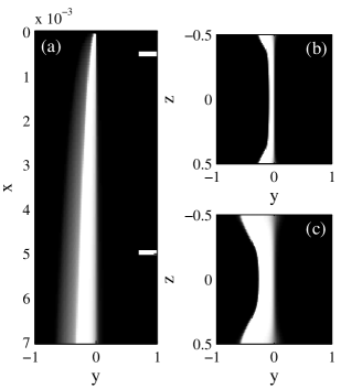
Figure 7: (a) concentration field $c$ of the product C averaged over the height of the microchannel in the case of a chemical reaction described by Eqs. (27) with $\chi=0.3$, $\beta=\sqrt{200}$, and $\gamma=0.0055$. (b-c) two slices $y$ vs. $z$ of the concentration of the product of the reaction, at the locations specified by white lines on (a).

in Ref. Ismagilov et al. (2000) ($D_{A}\approx 1.2\,10^{-9}$, $D_{B}\approx 10^{-10}$ m² s^-1, $a_{0}=1~{}$mM, $b_{0}=5~{}\mu$M, $K_{eq}=0.39~{}\mu$M). The depth-averaged concentration map $c$ in the microchannel is displayed in this figure (flow is downwards), together with two cross-sectional plots of the concentration in the ($y$,$z$) plane. As for the diffusion of a solute, the diffusion zone is not homogeneous over the height of the channel, due to the presence of the Poiseuille profile. Moreover, the diffusion zone is not symmetric ($x$,$y$), as a consequence of the stoechiometric imbalance ($\beta\neq 1$), and the asymmetry in diffusion coefficients ($\chi\neq 1$) Salmon et al. (2005b). The good agreement between the experimental shapes of the concentration profiles obtained in Ref. Ismagilov et al. (2000) and our simulation is clear. Moreover, the differences $\delta W$ between the widths of the interdiffusion zone at the wall and at $z=0$, are now consistent with the experimental data (for example, in Fig. 2 of Ref. Ismagilov et al. (2000), $\delta W\approx 0.1$–$0.3$, for $\text{Pe}\approx 12600$ and $x\approx$ 0.0001–0.001, our simulations give roughly the same results).

As above (see Figs. 3 and 4), we perform numerical simulations of Eqs. (27) over a wide range of $x$, and compute $w(x,z)$. The corresponding results are shown in Fig. 8, together with a map of the local exponents $\alpha(x,z)$, estimated by fitting the curves over a sliding decade of $x$ with a law $w(x,z)\sim x^{\alpha(x,z)}$ (in this case we have chosen $n=80$ and $p=40$ for the simulations).

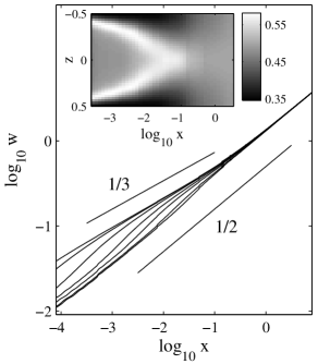
Figure 8: $\log_{10}(w)$ vs. $\log_{10}(x)$ for different $z$ in the case of Eqs. (27) with $\chi=0.3$, $\beta=\sqrt{200}$, and $\gamma=0.0055$. The two continous lines indicate the $1/2$ and $1/3$ power law behaviours. Insert: corresponding exponents $\alpha(x,z)$ vs. $\log_{10}(x)$ and $z$, obtained by local fits of $w$ vs. $x$ by power laws.

Obviously the phenomenology is very similar to that for the simple diffusion of a solute studied earlier: (i) close to the walls at $z=\pm 0.5$, $w\sim x^{1/3}$, whereas for $z\approx 0$, then $w\sim x^{1/2}$; (ii) beyond $x\approx 0.1$, the diffusion zone is homogeneous over the height of the channel and widens as $w\sim x^{1/2}$; (iii) close to the walls the sequence of power law regimes with exponents $1/2$, $1/3$, and $1/2$ is recovered; (iv) the locus of the transition from the $1/2$ to the 1/3 regime occurs earlier for $z$ closer to the walls. We find similar results when solving numerically Eqs. (27) for different set of parameters $\chi$, $\beta$ and $\gamma$. However, the increased complexity of the equations does not permit to perform as easily as in subsection II-D a simple analytical argument to formally argue for this phenomenology to hold whatever the values of the parameters. Theoretical approaches such as the ones described in Refs. Gálfi and Rácz (1988); Taitelbaum et al. (1992); Bazant and Stone (2000) may be useful to answer these questions.

IV Conclusion

The present numerical and theoretical study shows the generality of features reported for specific conditions by previous authors on lateral transport of solutes between streams in pressure-driven flows. For diffusion alone, the variations of the velocity along the thickness of the channel lead to remarkable features: while in the midplane of the microchannel the diffusive width classically grows with a $1/2$ exponent, close to the wall the broadening downstream can go through three power law regimes with exponents $1/2$, $1/3$ and $1/2$ again. Remarkably, our numerical computations suggest that this phenomenology may also hold for reaction-diffusion problems, at least in the diffusion-controlled limit of fast reaction kinetics. All our discussion and arguments, together with the various plots presented, are proposed in non-dimensional form, which hopefully should help experimentalists in assessing a priori the relevance of 3D effects in microfluidic experiments involving the lateral transport of solutes.