Intensity of Brillouin light scattering from spin waves in magnetic multilayers with noncollinear spin configurations: Theory and experiment

Abstract

The scattering of photons from spin waves (Brillouin light scattering – BLS) is a well-established technique for the study of layered magnetic systems. The information about the magnetic state and properties of the sample is contained in the frequency position, width, and intensity of the BLS peaks. Previously [Phys. Rev.  B 67, 184404 (2003)], we have shown that spin wave frequencies can be conveniently calculated within the ultrathin film approach, treating the intralayer exchange as an effective bilinear interlayer coupling between thin virtual sheets of the ferromagnetic layers. Here we give the consequent extension of this approach to the calculation of the Brillouin light scattering (BLS) peak intensities. Given the very close relation of the BLS cross-section to the magneto-optic Kerr effect (MOKE), the depth-resolved longitudinal and polar MOKE coefficients calculated numerically via the usual magneto-optic formalism can be employed in combination with the spin wave precessional amplitudes to calculate full BLS spectra for a given magnetic system. This approach allows an easy calculation of BLS intensities even for noncollinear spin configurations including the exchange modes. The formalism is applied to a Fe/Cr/Fe/Ag/Fe trilayer system with one antiferromagnetically coupling spacer (Cr). Good agreement with the experimental spectra is found for a wide variety of spin configurations.

Introduction

In a Brillouin light scattering (BLS) experiment spin waves in a magnetic system are probed via inelastic scattering of photons. The spin wave mode or magnon appears as a peak in the recorded spectrum, which is shifted by the magnon frequency $\nu_{m}$ relative to the central peak in the spectrum, which in turn is caused by elastically scattered photons. The shift reflects either an energy loss or energy gain corresponding to the creation (Stokes condition) or annihilation (anti-Stokes condition) of a magnon, respectively. The spectrum contains three different types of information: (i) the peak positions, which are determined by the spin wave frequencies, (ii) the peak shapes and especially their widths, which are related to the lifetime of the magnons, and (iii) the peak areas, which are proportional to the scattering cross-sections.

Most experiments focus on an analysis of the spin wave frequencies, which contain information about many magnetic properties such as, for instance, saturation magnetization, anisotropies, and interlayer coupling. With a suitable experimental geometry and procedure, these properties can be determined solely on the basis of the magnon frequencies. The peak width or linewidth contains information about the spin wave lifetime $\tau$ as it results in a linewidth broadening proportional to $1/\tau$. However, in most cases concerning epitaxial samples this magnon linewidth is much smaller than the apparatus broadening of about 1 GHz and cannot be resolved. Only when the magnon lifetime is strongly reduced, e.g. due to extrinsic two-magnon scattering in the case of exchange bias,PRB_63_214418 interlayer exchange coupling,JAP_93_3427 or in polycrystalline samples, the magnon linewidth becomes larger than the apparatus resolution and can be analyzed. On the other hand, the scattering intensities, which are the topic of this work, carry information mainly about the precessional amplitudes of the spin waves, but also depend on the optic and magneto-optic properties of the sample. For a full quantitative analysis of the BLS spectra, however, peak positions, line widths, and peak intensities have to be treated on an equal footing.

It is important to note that very few publications JPC_8_211 ; JAP_50_7784 ; PRB_18_4821 ; PRB_22_5420 ; JMMM_73_299 ; JAP_64_6092 ; JAP_69_5721 ; PRB_42_508 ; PRB_64_134406 ; PSS_196_16 ; PRB_53_2627 ; SS_454_880 ; SS_507_502 ; PRB_65_165406 ; PRB_63_104405 ; JMMM_290_530 have yet addressed the issue of the scattering intensities, although they contain valuable information about the mode types, the alignment of the magnetic moments and can even be used to investigate the magneto-optic coupling.PRB_63_104405 This lack of interest is probably due to the fact that the cross-sections cannot be easily analyzed in an intuitive manner, but require a comparison with theory. On the other hand, the kind of detailed information hidden in the peak intensities is of high relevance for many technological applications, such as data storage and communication technology, because the operation frequencies of contemporary magnetic devices approach the GHz regime, where the magnetization dynamics is closely related to the spin wave modes.

The computation of the scattering intensities is commonly considered to be very complicated.JMMM_73_299 There is only a handful of research groups, which have successfully developed and applied a suitable formalism, although the computation scheme is now known for more the three decades.JPC_8_211 Part of the computational complexity stems from the so-called partial waves approach,JMMM_73_299 ; JMMM_82_186 ; PRB_41_530 ; JMMM_145_278 which has been used to calculate the spin wave cross-sections in most publications. To our knowledge this approach has not yet been applied to and solved for noncollinear alignments of the magnetization and, thus, studies dealing with BLS intensities in noncollinear states are rarely available.PRB_42_508 ; PRB_53_2627 ; JMMM_290_530 However exactly those noncollinear states are crucial for the magnetization switching employed in a large number devices, such as for instance MRAM. A detailed understanding of the dynamics of noncollinear states is therefore highly desirable and a theoretical description of the spinwave properties of noncollinear states is of high technological relevance.

Only three publications PRB_42_508 ; PRB_64_134406 ; PRB_53_2627 employ the much easier ultrathin film approximation (UTFA),PRB_42_508 ; PRB_49_339 ; PRB_54_3385 ; JAP_84_958 which has been thought to be accurate only for the lowest-energy modes of ferromagnetic films with thicknesses well below the exchange length, i.e. a few nanometers in the case of Fe. However, in our previous work (Ref. PRB_67_184404, ) we have shown that the UTFA approach can be easily extended in order to accurately describe the modes in thicker films. We thereby included also the exchange modes and the twisted ground state found in exchange springs and also in the case of very strong interlayer exchange coupling. In the present contribution, we elucidate how this calculation scheme can be further extended to describe BLS cross-sections. In fact, the cross-section calculation using this method only requires a standard treatment of the light propagation in the multilayer apart from the formulae already presented in Ref. PRB_67_184404, . As we will show below, the optics involved is closely related to the magneto-optic Kerr effect (MOKE). This has the advantage that existing computer codes for the calculation of the MOKE can be reused to evaluate the BLS intensities.

Section I gives a detailed description of our computational procedure. In order to demonstrate the accuracy of the scheme we have recomputed the spectrum of Ref. JMMM_73_299, and find an excellent agreement with respect to the peak positions and intensities. An open-source computer program for the calculation of BLS frequencies, precessional amplitudes, and intensities (although excluding the ground state calculation) as well as for the calculation of MOKE can be downloaded from our server, see Ref. code, .

In Sec. II we apply our formalism to an well characterized epitaxial spin valve structure of the sequence Fe(14nm)/Cr(0.9 nm)/Fe(10 nm)/Ag(6 nm)/Fe(2 nm). While the bottom Fe/Cr/Fe trilayer couples antiferromagnetically, the top, thin Fe layer is decoupled and can be switched more easily by an external field. As a consequence this layer stack shows a rich variety of different spin configurations as a function of field strength and orientation. The application of BLS intensity theory to such a model system with multiple well defined spin configurations has to our knowledge been lacking yet. We find excellent agreement between our model calculation and the experimental spectra for all spin configurations.

I Calculation

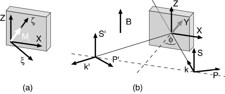
Figure 1: (a) Relation between the laboratory frame ($xyz$) and the coordinate system (${\xi}y{\zeta}$) attached to the static magnetization $M_{i}$ in each sheet. (b) Scattering geometry.

The calculation of the spin wave frequencies and scattering intensities is carried out based on our approach described in detail in Ref. PRB_67_184404, and requires only little additional programming effort. Only the standard formalism for the calculation of the MOKE in multilayers either using the full $4\times 4$ Yeh ; CJP_41_663 ; PRB_43_6423 or the approximate $2\times 2$ PRB_64_235421 matrix approach is needed in addition to the formalism in Ref. PRB_67_184404, . The computation is carried out in a sequence of four steps as explained in the following:

I.1 Calculation of the magnon frequencies

The calculation of the magnetic ground state and the spin wave frequencies in the extended UTFA is described in detail in Ref. PRB_67_184404, . In brief, the intralayer exchange within the ferromagnetic layers is treated as an effective bilinear interlayer coupling $J^{eff}_{1}$ between thin virtual sheets of the ferromagnetic material. The virtual multilayer consisting of the virtual ferromagnetic sheets is then treated within the conventional UTFA approach.PRB_42_508 ; PRB_49_339 ; PRB_54_3385 ; JAP_84_958 It is of crucial importance to divide the ferromagnetic layers into thin enough sheets in order to obtain (i) the correct ground state for the case of strong interlayer coupling or (ii) the frequencies of modes, which are not uniform in the perpendicular direction, i.e. Damon-Eshbach modes, optic and exchange modes. In particular, an improper ground state configuration can lead to the disappearance of some modes, especially the optic modes in antiferromagnetically coupled systems.

I.2 Calculation of the precessional amplitudes

The calculation of the mode profiles is straightforward. For a multilayer with $N$ sheets, the numerical procedure consists of solving the set of $2N$ equations given by Eq. (A2) in Ref. PRB_67_184404, for the dynamic magnetization components $m_{i,k}$ of each mode with index $n$ and corresponding frequency $\omega_{n}$:

$$\sum_{i,k}A_{j,l}^{i,k}(\omega_{n})m_{i,k}=0,$$ (1)

where $i,l$ are sheet indices ($i,l=1\ldots N$) and $k,l$ are axis indices ($k,l=y,\xi$). The relation between the laboratory frame ($xyz$) and the coordinate system (${\xi}y{\zeta}$) attached to the static magnetization $M_{i}$ in each sheet is shown in Fig. 1(a). This calculation can be easily carried out with standard matrix algorithms, e.g. from Ref. nr, .

I.3 Normalization of the precessional amplitudes

In order to calculate the relative scattering intensities the amplitude of each spin wave mode has to be normalized such that its energy per unit area is equal to the thermal energy. For low frequency modes ($\hbar\omega\ll kT$), which are of relevance for the present case, the thermal energy is just $kT$. Therefore, the mode amplitudes have to be adjusted so that they have the same energy. The mean energy per unit area stored in a mode is given by

$$E(\vec{m}_{i})=\frac{1}{2}\sum_{i,j}\Bigl{[}\frac{\partial^{2}F}{\partial m_{i,y}\partial m_{j,y}}m_{i,y}m_{j,y}$$

$$+\frac{\partial^{2}F}{\partial m_{i,\xi}\partial m_{j,\xi}}m_{i,\xi}m_{j,\xi}\Bigr{]},$$ (2)

where $F$ is the magnetic free energy per unit area and $\vec{m}_{i}$ is the dynamic magnetization per unit area inside sheet $i$. Fortunately the matrix elements $A_{j,l}^{i,k}$ are proportional to the second derivatives of the free energy,

$$A_{i,\xi}^{j,y}=\frac{1}{M_{j}d_{j}}\quad\frac{\partial^{2}F}{\partial m_{i,y}\partial m_{j,y}}$$ (3)

$$A_{i,y}^{j,\xi}=\frac{1}{M_{j}d_{j}}\quad\frac{\partial^{2}F}{\partial m_{i,\xi}\partial m_{j,\xi}}.$$ (4)

The mode energy normalization is thus performed via scaling $\vec{m}_{i}$ by $1/\sqrt{E(\vec{m}_{i})}$.

I.4 Calculation of the scattering intensities

In the next step the interaction of the spin waves with the electromagnetic wave via the magneto-optic coupling has to be taken into account. The spin wave induces a polarization $\Delta\vec{P}_{i}$ inside sheet $i$ oscillating at $\omega_{Light}\pm\omega_{SW}$:JMMM_73_299

$$\Delta\vec{P}_{i}=\Delta\epsilon_{i}\vec{E}_{i}=\frac{1}{2}K_{i}\vec{E}_{i}\times\vec{m}_{i},$$ (5)

where $\Delta\epsilon_{i}$ is the magnetic part of the dielectric tensor, $K_{i}$ is the linear magneto-optic coupling constant, $\vec{E}_{i}$ is the electric field of the light, and $\vec{m}_{i}$ is the dynamic magnetization, each inside the magnetic sheet with index $i$. Only the first order magneto-optic coupling or terms linear in $m$ have been taken into account. The phase of the dynamic magnetization has to be considered, which means $\vec{m}$ is a complex vector with e.g. imaginary out-of plane component $m_{y}$ and real in-plane component $m_{\xi}$ as assumed in Ref. PRB_67_184404, .note It is worth noting that exactly the same formula (5) can also be used to calculate the MOKE signal in the approximative $2\times 2$ matrix approach of Ref. PRB_64_235421, . The only difference between Eq. (4.3) in Ref. PRB_64_235421, and Eq. (5) is the factor $1/2$ and the use of the static instead of the dynamic magnetization. In both cases of BLS and MOKE, the electromagnetic wave generated by the induced polarization $\Delta\vec{P}$ has to be equated taking into account the dielectric tensors and standard boundary conditions of all sheets. The procedure is exactly the same for the reflected and the $180^{\circ}$ backscattered light. The only difference is that the reflected light propagates along the $\pm\vec{k}^{\prime}$ directions, while the $180^{\circ}$ backscattered light propagates along the $\pm\vec{k}$ directions [see Fig. 1(b)] corresponding to a reversed sign of the in-plane component of the wavevector.

In the case of MOKE it is well known that the resulting complex Kerr angle, e.g. for incident s-polarization $\Phi_{s}=E^{\prime}_{p}/E^{\prime}_{s}=r_{sp}/r_{ss}$ can be expanded as a function of the Cartesian magnetization components:JAP_91_7293

$$\Phi_{s}=\sum_{i}\Bigr{[}r_{sp,(M=0)}+L_{i}m_{i,x}+P_{i}m_{i,y}+O(m^{2})\Bigl{]}/r_{ss},$$ (6)

where the diagonal reflection coefficient $r_{ss}$ is independent of the magnetization, and the nonmagnetic part of the off-diagonal reflection coefficient $r_{sp,(M=0)}$ is zero for materials with cubic symmetry. Terms quadratic in $m$ are known to be small unless the angle of incidence is nearly perpendicular or grazing. Terms linear in the transversal magnetization component $m_{z}$ only appear, if the incident light has p-polarized components.

From the above discussion it is clear that the intensity of the scattered light from each mode with index $n$ can also be decomposed in the same way as in Eq. (6):

$$I^{(n)}=\left|E^{(n)}_{BLS}\right|^{2}=\frac{I_{0}}{4}\left|\sum_{i}(L^{BLS}_{i}m_{x,i}^{(n)}+P^{BLS}_{i}m_{y,i}^{(n)})\right|^{2}.$$ (7)

Equations (7) and (6) can easily be deduced employing the approximate magneto-optic formalism in Ref. PRB_64_235421, . Additionally, it can be shown that the coefficients $L$ and $P$ in Eqs. (6) and (7) in fact only differ by sign. This is also plausible from simple symmetry considerations: Neglecting the small Kerr component and assuming s-polarization of the incident light the electric field vector is parallel to the $z$-direction everywhere. Therefore, the polar magnetization component $m_{y}$ results in a Kerr component with electric field vector parallel to $\Delta P\propto E_{z}\times m_{y}$, that is parallel to the $x$-direction. As the projection of $\hat{x}$ on the $P$ and $P^{\prime}$ directions is the same [see Fig. 1(b)], the polar coefficient must be the same for reflection and backscattering, i.e. $P_{BLS}=P_{MOKE}$. On the other hand, the longitudinal magnetization component $m_{x}$ results in an electric field vector of the Kerr component parallel to the $y$-direction. As can be seen from Fig. 1 (b) the projections of the $y$-direction on $P$ and $P^{\prime}$ only differ in sign. Therefore, the longitudinal coefficient has opposite sign for the $180^{\circ}$ backscattering configuration, i.e. $L_{BLS}=-L_{MOKE}$. The arguments are more involved in the case of incident p-polarization. However, it is well-known from theory that the first-order intensities are the same for sp and ps scattering.PRB_64_134406 In summary, the BLS scattering intensities in the $180^{\circ}$ backscattering configuration can be calculated in the following way:

$$I^{(n)}\propto\left|\sum_{i}(-L^{MOKE}_{i}m_{x,i}^{(n)}+P^{MOKE}_{i}m_{y,i}^{(n)})\right|^{2},$$ (8)

where the dynamic magnetization of each spin wave mode $n$ has to be computed and normalized as described above, and $L_{i}$ and $P_{i}$ are the effective longitudinal and polar MOKE coefficients of layer $i$ as defined by Eq. (6). They can be calculated using the standard $4\times 4$ formalism as explained in Refs. Yeh, ; CJP_41_663, ; PRB_43_6423, or even more easily with the approximative $2\times 2$ approach presented in Ref. PRB_64_235421, .

I.5 Comparison with the theory of Cochran and Dutcher

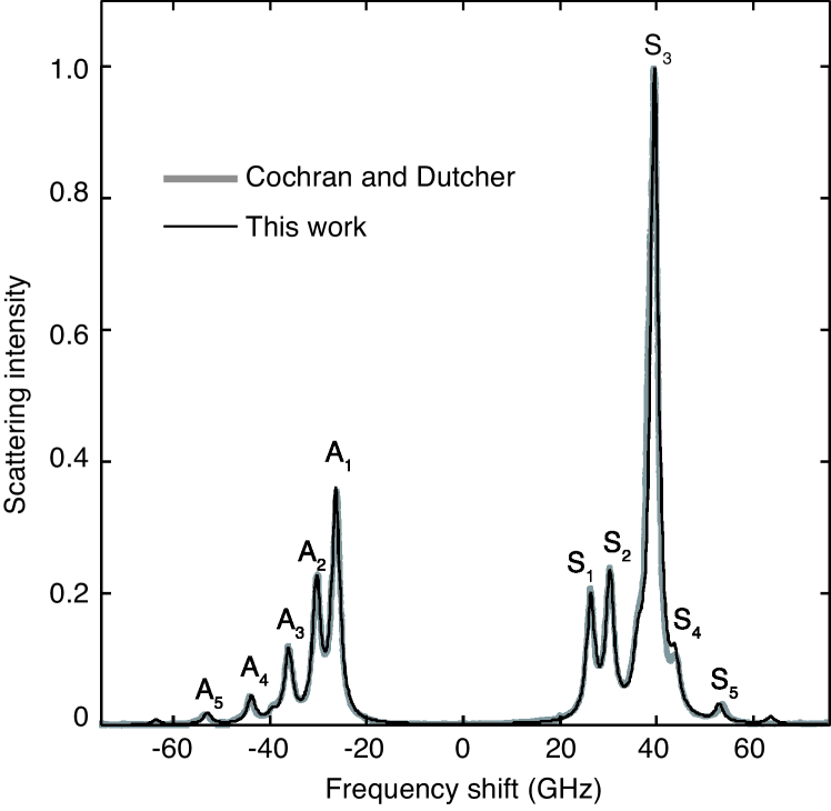
Figure 2: Calculated spectrum of a 85 nm-thick Fe layer (black) in comparison with the spectrum calculated by Cochran and Dutcher (grey) reproduced with permission from Fig. 2(a) in Ref. JMMM_73_299, .

In order to check the reliability and accuracy of the calculational scheme described above, we have calculated the relative intensities of a thick iron film on a Au substrate using the same parameters as given by Cochran and Dutcher in Ref. JMMM_73_299, . The parameters for the Fe film are: thickness 85 nm, saturation magnetization $M_{S}=1.68$ MA/m, exchange constant $A=1.8\times 10^{-11}$ J/m, gyromagnetic ratio $\gamma/2\pi=29.26$ GHz/T, and refraction index $n_{Fe}=2.83+2.90i$. For the Au substrate we use a refraction index $n_{Au}=0.67+2.05i$. The sample is saturated in an external field of $0.3$ T applied perpendicular to the plane of incidence and parallel to the film plane [Fig. 1(b)]. The light wavelength of 514.5 nm and the angle of incidence of $45^{\circ}$ results in an in-plane magnon vector of $1.73\times 10^{7}$ m^-1. The absolute value of the magneto-optic coupling or the presence of a thin capping layer (as usually the case in experimental studies) are of minor importance as they merely scale the absolute value of all intensities, while the spectra are anyway normalized to a maximum intensity of 1 for the anti-Stokes Damon-Eshbach mode labelled $S_{3}$.

In order to obtain accurate results the layer has been virtually divided into 85 sheets each 1 nm thick. As in Ref. JMMM_73_299, the calculated spectrum is convoluted with a Lorentzian lineshape with a full width at half maximum (FWHM) of 2 GHz, which corresponds to a typical instrumental function of a BLS experiment. The results of our calculation are shown in Fig. 2 and compared with the spectrum of Cochran and Dutcher.JMMM_73_299 The agreement is excellent and the two spectra can hardly be distinguished. Only the modes A4, A5, S4 and S5 differ slightly in frequency by approximately 1 GHz. This small deviation should not arise from using the extended UTFA, which only slightly overestimates (less than 0.2 GHz) the frequency of the highest modes as compared to the partial waves method. It might, however, be due to the fact that we used the magnetostatic approximation, i.e. we did not take into account the electric high-frequency conductivity in our spin wave calculation. This will cause some error for films with thicknesses comparable or larger than the skin depth at the spin wave frequency.

II Application to a coupled trilayer system

In this section, we apply the formalism described in Sec. I to a multilayer structure with three ferromagnetic layers, which are subject to competing interactions and thus show a rich variety of spin configurations as a function of the external field.

II.1 Sample preparation and experimental setup

Epitaxial Fe(14 nm)/Cr(0.9 nm)/Fe(10 nm)/Ag(6 nm)/ Fe(2 nm) spin valve structures have been prepared by molecular beam epitaxy on top of a GaAs/Ag(001) buffer system. The samples have been capped with a 50 nm-thick antireflection ZnS layer in order to prevent oxidation and enhance the magneto-optic response. This kind of structures are interesting model systems, which we are also employing to investigate current-induced magnetization switching.arxiv The preparation is described in detail elsewhere.arxiv The Cr thickness has been chosen in order to obtain a strong antiferromagnetic coupling in the bottom Fe/Cr/Fe trilayer, which fixes the center reference layer. The top, thin Fe layer is decoupled and can be switched more easily by an external field or a perpendicularly applied current. As the samples are fully epitaxial and therefore mainly in a magnetic single domain state the remagnetization behavior can be modeled easily. However, as a consequence of the various competing interactions – Zeeman energy, magnetocrystalline anisotropy of all ferromagnetic layers, interlayer exchange coupling – a rich variety of different magnetization configurations is possible and hysteretic effects determine which configurations actually occur at low fields.

The BLS spectra have been recorded using a Sandercock type ($2\times 3$) pass tandem Fabry-Pérot interferometer TAP_51_173 in the $180^{\circ}$ backscattering geometry. The wavelength $\lambda=532$ nm of the laser light together with the angle of incidence of 45^∘ results in an in-plane magnon wave vector $q=1.67\times 10^{7}$ m^-1 of the measured magnons. The external field was applied in the film plane and perpendicular to the magnon wave vector as sketched in Fig. 1(b).

II.2 Results and discussion

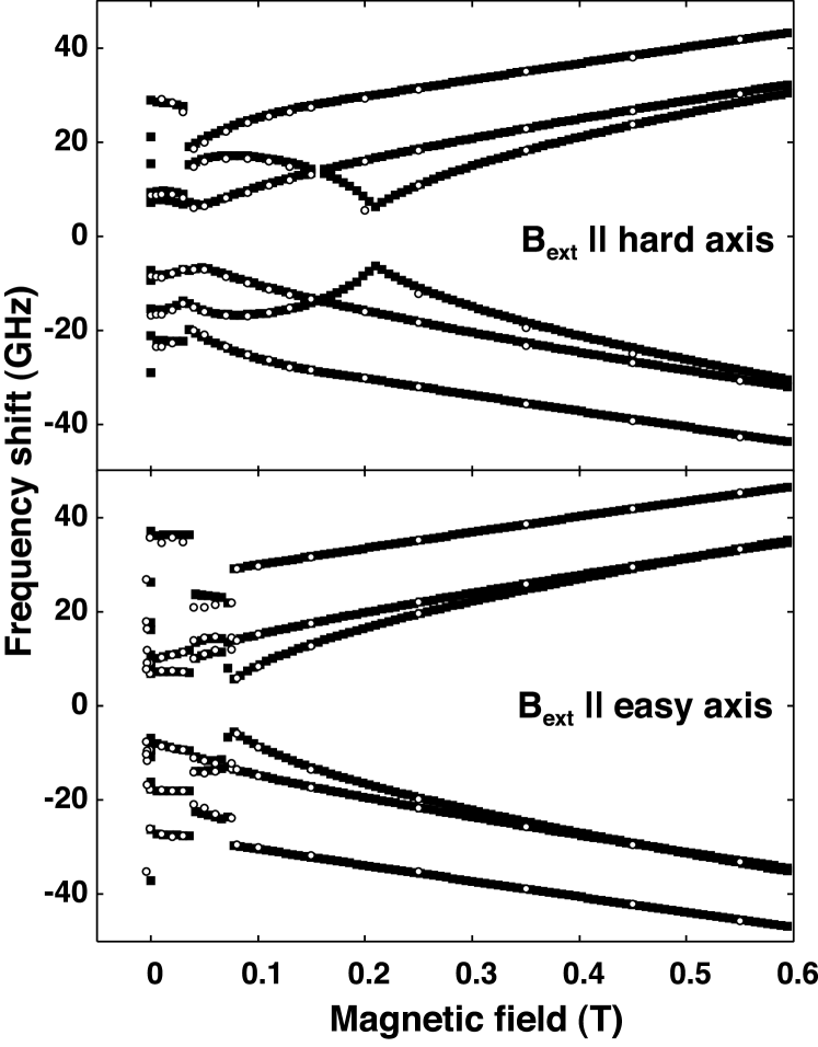
Figure 3: Field dependence of measured BLS data (open circles) and least square fit (solid line) of a Fe(14 nm)/Cr(0.9 nm)/Fe(10 nm)/Au(6 nm)/Fe(2 nm) sample.

Figure 3 shows the experimental spin wave frequencies (open circles) as a function of the external field applied parallel to the easy [001] (bottom graph) and hard [011] direction (top graph) of the cubic magnetocrystalline anisotropy. Corresponding spectra are shown in Fig. 5 below. Only the three dipolar modes, which are lowest in frequency, are shown. These modes can be classified as one acoustic and two optical modes. This classification, however, is strictly valid only for the saturated sample. The acoustic mode is characterized by an in-phase precession of the magnetization in all layers, while for the optical modes the precession of at least two neighboring layer magnetizations is out-of-phase. The graphs can be divided into three distinct field regions bounded by switching events: For low field values ($B_{ext}<35$ mT) there is a distinct asymmetry between the Stokes and the anti-Stokes side. This unique feature proves an antiparallel alignment of the magnetic moments of the two bottommost Fe layers collinear with the external field applied in easy axis direction.PRL_57_2442 At higher fields ($B_{ext}>35$ mT) the antiferromagnetically coupled bottom Fe/Cr/Fe double layer switches into a canted configuration with a relative angle between the layers magnetizations of about $90^{\circ}$. This so-called spin-flop transition is a first order transition and can be distinguished by a discontinuity (jump) of the mode frequencies. The sample saturates at an external field of about 80 and 180 mT in the easy and hard axis configuration, respectively. As the coupling and anisotropy energies are of comparable magnitude, magnetic saturation is a first order transition marked by jumps in the frequencies for the easy axis configuration. On the other hand, in the hard axis configuration the saturation is approached continuously, i.e., following a second order transition. In this case no jumps in the mode frequencies can be observed. The saturation point is only marked by a minimum in the lowest mode frequency, which is the optical mode of the antiferromagnetically coupled Fe/Cr/Fe double layer, and a weak change in slope of the other modes.

The hard and easy axis data have been fitted simultaneously in order to extract the magnetic parameters of the Fe layers and the interlayer coupling. In order to reduce the number of adjustable parameters the intralayer exchange stiffness and gyromagnetic ratio have been fixed to their literature values of $D=2.4\times 10^{-17}$ Tm² and $\gamma/2\pi=29.4$ GHz, respectively. The bottom (index $b$) and central (index $c$) layers have been assumed to have equal saturation magnetizations $M_{S(b,c)}$ and cubic anisotropies $K_{C(b,c)}$, and the perpendicular interface anisotropies have been assumed to be the same for the three chemically similar Fe/Ag and Fe/Au interfaces, $K_{S(Au,Ag)}$. $K_{S(Cr)}$ is the interface anisotropy of the two Fe/Cr interfaces and $K_{S(ZnS)}$ of the topmost Fe/ZnS interface.

From the very low switching field of the top layer (index $t$) of less than 1 mT when the field direction is reversed (see in Fig. 4 below), we can conclude that the interlayer exchange coupling across the 6 nm-thick Ag interlayer is negligibly small. Therefore, it has been set to zero. In order to properly describe the modes a division of all three ferromagnetic layers in $1$ nm-thick sheets has been employed. This is sufficient to take care of the partial nonuniformity of the modes in the $y$-direction and of the twist of the static magnetization, which is almost negligible for the easy axis configuration, yet has some influence on the hard axis configuration. The parameters extracted from the fit are: $M_{S(b,c)}=1.76$ MA/m, $M_{S(t)}=1.58$ MA/m, $K_{C(b,c)}=57$ kJ/m³, $K_{C(t)}=33$ kJ/m³, $K_{S(Au,Ag)}=0.5$ mJ/m², $K_{S(Cr)}=0.0$ mJ/m², $K_{S(ZnS)}=0.3\,$mJ/m², and a strength of the bilinear and biquadratic coupling contributions across Cr of $J_{1}=-0.97$ mJ/m² and $J_{2}=-0.10$ mJ/m², respectively. The calculated field dependences using these parameters are plotted as solid lines in Fig. 3. As can be seen, the results of the calculation are in excellent overall agreement with the experimental data. Only the highest frequency mode differs somehow in the canted state for the easy axis configuration. This small discrepancy could be due to either the too simplified $J_{1}$-$J_{2}$ model used to describe the coupling. It has been shown to be possibly insufficient to describe the coupling across Cr spacers, kholin . Another reason could be the necessary reduction of the huge number of fitting parameters. We also point out the notable asymmetry between Stokes and anti-Stokes frequencies in the saturated state, especially of the lowest optic modes in the hard axis configuration, which could not be fully reproduced by the fit. It is known that such an asymmetry can stem from asymmetric interface anisotropies,PRB_41_530 , which could not be properly taken into account in the calculation as the large number of at least six interface anisotropy parameters (one for each interface) is very cumbersome to fit.

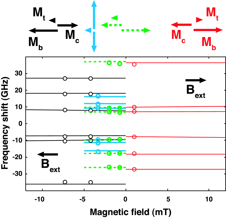
Figure 4: Field dependence of measured (open circles) and calculated (solid and dashed lines) frequencies at low fields. The field is swept form positive to negative values. The colors of the calculated curves correspond to the magnetization alignments shown in the upper part.

While an applied external field will tend to align the thickest bottom layer and the thinnest uncoupled top layer in the field direction and, thus, fix the magnetization directions of all layers in the antiferromagnetic state in easy axis configuration, the situation gets much more complex when the field approaches the zero value. In zero external field four directions of the magnetizations of the coupled bottom double layer and four directions of the magnetizations of the uncoupled top layer, each parallel to an easy axis, are possible. However, only nine out of these 16 possible zero field ground states can be distinguished by the theory and the experimental setup used here, as a reversal of the sign of the $x$-components of the static magnetization of either the coupled double layer or the free top layer, i.e. transversal to the external field direction, has neither an effect on the frequencies nor the BLS intensities due to linear magneto-optic coupling. The reason is that as a result only the sign of the $z$-components of the precessional amplitudes changes. However, they mediate neither dynamic dipolar coupling as can be concluded form Eq. (A8) in Ref. PRB_67_184404, , nor a magneto-optical response as $m_{z}$ does not enter Eq. (8). The intensities only depend on $m_{z}$ via the second order magneto-optic coupling, which has been neglected in Eq. (8), as it has only a small impact on the intensities for our setup with a large angle of incidence.

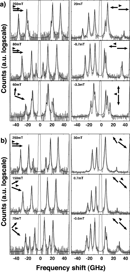
Figure 5: Experimental (thick grey lines) and calculated (thin black lines) BLS spectra at different fields applied along the easy (a) and hard (b) axis of the magnetocrystalline anisotropy. The computed directions of the magnetic moments of the layers are indicated with arrows similar to those in Fig. 4.

In Fig. 4 we show the experimental (open circles) and calculated frequencies (solid and dashed lines) at low field ($B_{ext}<10$ mT). To take into account the switching events, the field has been scanned from positive to negative values and applied parallel to an easy direction. As the Zeeman energy has a negligible influence on the spin waves at such low field values, the differences in frequency must be mainly due to different alignments of the static magnetization vectors. Four different ground states with corresponding transitions at about -0.3, -3, and -3.5 mT can be observed. By comparing the calculated and experimental frequencies the following remagnetization behavior can be derived: At zero field the thickest, bottommost layer points in the positive field direction and the other layers are antiparallel to their nearest neighbor (red state). At a small reversed field of about $-0.3$ mT the thin top layer switches into the field direction (green state). Then at about $-3$ mT the magnetizations of the bottom double layer, initially aligned with its net magnetic moment ($M_{b}-M_{c}$) along the field direction, switches first into the direction perpendicular to the external field (blue state) and then completely reverses at about $-3.5$ mT (black state). The about an order of magnitude larger switching field of the coupled double layer as compared to the single layer can be explained by a competition between the pinning energy, which is proportional to the thickness, and the Zeeman energy, which is proportional to the net magnetic moment.

While such a remagnetization sequence can be easily examined also with integrating static methods as, for instance, MOKE or SQUID magnetometry, the analysis of the peak areas and widths in the BLS spectra also allows one to determine whether the sample is in a single or multiple domain state. A multiple domain configuration can be recognized by a line broadening and altered intensities for small domains mediating two-magnon scattering or multiple peaks for large enough domains. Experimental spectra for the easy and hard axis configuration are shown as grey curves in Fig. 5. Calculated spectra based on the parameters extracted from the fit are plotted as thin black lines. For the intensity calculations we have only used the magnetic parameters extracted from the fit in Fig. 3, and literature values CRC_HANDBOOK for the indices of refraction of the layers, intrapolated to our laser wavelength: $n_{Ag}=0.248+i3.392$, $n_{Fe}=2.595+i3.322$, and $n_{Cr}=2.833+i4.450$. The ZnS capping layer, which has only a minor influence on the spectra has been neglected. As the experimental FWHMs of all peaks have approximately the same value of about 1 GHz, which is the resolution of the spectrometer, we have assumed a Lorentzian lineshape with this linewidth for the calculation of the spectra. The background level and the absolute intensity have been adjusted manually in order to match the experimental spectra. The surprisingly good overall agreement of the calculated intensities may be ascribed to the following facts: (i) the indices of refraction of the employed materials are rather well known, (ii) the optic properties of the capping layer, which are always somehow uncertain due to interaction with the ambient air, e.g. oxidation, moisture etc. have little influence on the spectra, and (iii) the less well known magneto-optic coupling parameters play a negligible role as long as they are the same for all Fe layers. On the other hand, the good agreement of both the frequencies (Fig. 4) as well as the entire spectra (Fig. 5) proves that the theory well describes the spin wave properties. Hence, the calculated mode profiles are close to the actual situation in the sample, and the sample is indeed in a single domain ground state close to the computed one.

III Conclusions

We have developed a formalism for the quantitative interpretation of BLS intensities. A specific emphasis is laid on multilayers with non-collinear alignment of the layer magnetizations and/or non-homogeneous layer magnetization profiles in the direction perpendicular to the layers, for instance, canted magnetization alignments, twisted spin-configurations, or exchange modes. The method combines our previously presented EUTFA approach with standard MOKE modelling and should work properly for a total thickness of the layer stack of up to some 100  nm and in the frequency range of up to some 100 GHz accessible to BLS. Although the algebra involved is not very demanding, a computer program is needed to determine the BLS frequencies, mode-profiles, and intensities. We make the source code freely available code in order to encourage other researchers to analyze the BLS intensities of their experimental spectra.

In order to show the accuracy of the formalism we have recalculated spectra of a single, saturated Fe layer and compare it with previous calculations. In the experimental part we have demonstrated that BLS spectra recorded from multilayers with three Fe layers can be described accurately by our formalism for a large variety of spin-configurations. In fact, we find excellent agreement in all cases. Although it is clear that the well known theory of BLS should be able to describe the cross sections in noncollinear configurations, experimental evidence utilizing a well characterized model system to our knowledge has been left undone so far.

The method described here should also be easily extendable to include out-of-plane spin-configurations and second order magneto-optic coupling, which have not yet been taken into account in this work. The method is well suited to gain technologically relevant, quantitative information about spinwave mode types, the alignment of the magnetic moments, and the magneto-optic coupling.

References

- (1) Electronic mail: m.buchmeier@fz-juelich.de
- (2) S. M. Rezende, A. Azevedo, M. A. Lucena and F. M. de Aguiar, Phys. Rev. B 63, 214418 (2001).
- (3) B. K. Kuanr et al, J. Appl. Phys. 93, 3427 (2003).
- (4) W. Wettling, M. G. Cottam and J. R. Sandercock, J. Phys. C: Solid State Phys. 8, 211 (1975).
- (5) W. Wettling and J. R. Sandercock, J. Appl. Phys. 50, 7784 (1979).
- (6) R. E. Camley and D. L. Mills, Phys. Rev. B 18, 4821 (1978).
- (7) R. E. Camley and M. Grimsditch, Phys. Rev. B 22, 5420 (1980).
- (8) J. F. Cochran, and J. R. Dutcher, J. Magn. Magn. Mater. 73, 299 (1988).
- (9) J. F. Cochran, and J. R. Dutcher, J. Appl. Phys. 64, 6092 (1988)
- (10) H. Moosmtiller, J. FL Truedson, and C. E. Patton, J. Appl. Phys. 69, 5721 (1991).
- (11) J. F. Cochran et al., Phys. Rev. B 42, 508 (1990).
- (12) J. Cochran, Phys. Rev. B 64,134406 (2001).
- (13) G. Gubbiotti, G. Carlotti, L Giovannini, and L. Smardz, Phys. stat. sol. (a) 196, 16 (2003).
- (14) R. W. Wang, D. L. Mills, Eric E. Fullerton, Sudha Kumar, and M. Grimsditch, Phys. Rev. B 53, 2627 (1996).
- (15) P. Vavassori, M. Grimsditch, E. E. Fullerton, L. Giovannini, R. Zivieri and F. Nizzoli, Surf. Science 454, 880 (2000).
- (16) R. Zivieri, P. Vavassori, L. Giovannini, F. Nizzoli, E. E. Fullerton and M. Grimsditch, Surf. Science 507, 502 (2003).
- (17) R. Zivieri, P. Vavassori, L. Giovannini, F. Nizzoli, E. E. Fullerton, M. Grimsditch and V. Metlushko, Phys. Rev. B 65, 165406 (2002).
- (18) L. Giovannini, R. Zivieri, G. Gubbiotti, G. Carlotti, L. Pareti and G. Turilli, Phys. Rev. B 63, 104405 (2001).
- (19) D.C. Crew, R.L. Stamps, H.Y. Liu, Z.K. Wang, M.H. Kuok, S.C. Ng, K. Barmak, J. Kim and L.H. Lewis, J. Magn. Magn. Mater. 290, 530 (2005).
- (20) J. Barnas and P. Grünberg, J. Magn. Magn. Mater. 82, 186 (1989).
- (21) B. Hillebrands, Phys. Rev. B 41, 530 (1990).
- (22) R. J. Hicken, D. E. P. Eley, M. Gester, S. J. Gray, C. Daboo, A. J. R. Ives and J. A. C. Bland, J. Magn. Magn. Mater. 145, 278 (1995).
- (23) R. L. Stamps, Phys. Rev. B 49, 339 (1994).
- (24) M. Grimsditch, S. Kumar and E. E. Fullerton, Phys. Rev. B 54, 3385 (1996).
- (25) S.M. Rezende et al., J. Appl. Phys. 84, 958 (1998).
- (26) M. Buchmeier, B. K. Kuanr, R. R. Gareev, D. E. Bürgler and P. Grünberg, Phys. Rev. B 67, 184404 (2003).
- (27) http://www.fz-juelich.de/iff/e_iee_research_4a1/
- (28) P. Yeh, Surf. Sci.96, 41 (1980).
- (29) S. Visnovsky, Czech. J. Phys. 41, 663 (1991).
- (30) J. Zak, E. R. Moog, C. Liu and S. D. Bader, Phys. Rev. B 43, 6423 (1991).
- (31) P. Bertrand, C. Hermann, G. Lampel, and J. Peretti, Phys. Rev. B 64, 235421 (2001).
- (32) Numerical Recipes in C, Cambridge University Press (2001), http://www.nr.com.
- (33) In some publications, e.g. Ref. JMMM_73_299, , the complex conjugate of is used for the anti-Stokes components, which however come about automatically when using negative anti-Stokes frequencies as in Ref. PRB_67_184404, .
- (34) K. Postava et al. J. Appl. Phys.91, 7293 (2002).
- (35) H. Dassow, R. Lehndorff, D. E. Bürgler, M. Buchmeier, P. A. Grünberg, C. M. Schneider and A. van der Hart, J. Appl. Phys. 89, 222511 (2006).
- (36) J. R. Sandercock, Topics in Applied Physics 51, 173 (1982).
- (37) P. Grünberg, R. Schreiber, Y. Pang, M. B. Brodsky and H. Sowers, Phys. Rev. Lett. 57, 2442 (1986).
- (38) N. M. Kreines, D. I. Kholin, S. O. Demokritov and M. Rikart, JETP Lett. 78, 627 (2003).
- (39) Handbook of Chemistry and Physics, 82nd ed., CRC Press 2001-2002.