Robustness of adiabatic passage through a quantum phase transition
Abstract
We analyze the crossing of a quantum critical point based on exact results for the transverse XY model. In dependence of the change rate of the driving field, the evolution of the ground state is studied while the transverse magnetic field is tuned through the critical point with a linear ramping. The excitation probability is obtained exactly and is compared to previous studies and to the Landau-Zener formula, a long time solution for non-adiabatic transitions in two-level systems. The exact time dependence of the excitations density in the system allows to identify the adiabatic and diabatic regions during the sweep and to study the mesoscopic fluctuations of the excitations. The effect of white noise is investigated, where the critical point transmutes into a non-hermitian “degenerate region”. Besides an overall increase of the excitations during and at the end of the sweep, the most destructive effect of the noise is the decay of the state purity that is enhanced by the passage through the degenerate region.
pacs:
73.43.Nq 05.40.-a 75.10.Jm1 Introduction
Adiabatic passages are a fascinating and important tool in modern physics, since they allow to manipulate quantum states in a controlled manner via tunable parameters of a physical model system. Their potential impact ranges from setting current standards by means of adiabatically pumping charge through a quantum dot[1, 2, 3, 4] to the access to ground states of e.g. non-integrable Hamiltonians via adiabatically connecting to it from an integrable Hamiltonian[5]. Since modern methods in quantum optics allow fabrication of a wide class of lattice Hamiltonians with systems of atoms loaded into a suitably engineered optical trap, these techniques have become experimentally accessible nowadays. We here will discuss the latter application of a possibly adiabatic transit of a ground state with an explicit time dependent Hamiltonian and “slowly” varying parameters, which in the recent literature has also been termed adiabatic quantum computation (AQC)[5]. The efficiency of this procedure is compromised by size effects and by the presence of noise, the arch-enemy of all quantum information tasks.
The closing of the gap in the spectrum of excitations with growing system size gives a limit to the rate the parameters may be changed in order to have a sufficiently high fidelity with the ground state of the final Hamiltonian. In other words, the gap rules the time of computation. An intriguing question is then, what happened if a quantum critical point[6] is crossed during the passage. In the dynamic scenario presented here, the vanishing gap makes the notion of slow change rates obsolete, and strictly speaking no adiabatic passage exists across a quantum critical point. In the laboratory we have to deal with finite systems and as a consequence the gap, though scaling down to zero somehow with the system size, will nevertheless be finite. Then, the question arises how the fidelity of the ground state and/or the time of computation scales with the system size. This question is relevant for deciding whether adiabatic quantum computation may be successful or not. It has been addressed for the one-dimensional transverse Ising and the anisotropic Heisenberg-chain[8] in numerically solving the Heisenberg equation; the excitation probability has been calculated perturbatively taking into account a finite number of multiparticle excitations. The authors concluded that the adiabatic time scale for the Ising model in a transverse field scales polynomially with the system size. Besides a complete treatment of many-particle excitations this work did not take into consideration the crucial role fluctuations of the average excitation number play in particular for small system size. The previous question is also related to the Kibble-Zurek theory, where critical scaling laws have been employed to obtain predictions for the density of defects after the crossing of a real phase transition[10, 11, 12]. Its predictions have been tested for the one-dimensional transverse Ising model in Ref. [9], where the kink density has been calculated numerically and good qualitative agreement with the Kibble-Zurek scenario has been reported up to little quantitative discrepancy. By means of simple scaling arguments the density of created excitations as function of the sweeping rate has been evaluated for models belonging to different universality classes[13]. Using the exact solution for the transverse Ising model [7, 14, 15, 16], the kink density at vanishing magnetic field has been calculated in Ref. [17], and numerical discrepancies with Ref. [9] have been noted, where the time dependent Bogoliubov approach has been applied and excitation probabilities in the long time limit are obtained from a mapping to Landau-Zener tunneling.
How the presence of the noise affects this scenario is a rather unexplored, though very important, topic. In experimental setups one has to struggle with the influence of environmental degrees of freedom. This transforms the avoided criticality of the finite system into a region of non-hermitian degeneracy[18] extending over a finite interval in control parameter space. This means that the system passes through a gapless phase within a finite time window. Moreover, besides the inverse of the spectral gap that sets a lower bound on the sweeping period, the noise introduces a second time scale: the dephasing time, that on the contrary sets an upper bound. These competing time scales give rise to non-trivial effects, which are largely ignored in the recent literature on AQC [19, 20, 21] notwithstanding their importance for a realistic analysis of AQC protocols.
A prominent and simple class of models with quantum critical point are the one dimensional XY models in transverse magnetic field[6, 7]. In this work, we trace the exact evolution of the model during a sweep in order to study the robustness of the adiabatic passage against size effects with and without the presence of noise in the driving field. The paper is organized as follows: In section 2 we present the model Hamiltonian together with a sketch of its exact solution of the dynamics and we briefly review the Kibble-Zurek scenario for a quantum phase transition in section 3. In section 4, the results for the excitation probability and its mean square fluctuations during the sweep are presented and discussed. In section 5, we analyze the case of a noisy driving field. Conclusions out of our findings are drawn in section 6.
2 The model and its exact solution
The model Hamiltonian under consideration throughout this work is the one-dimensional spin-1/2 XY model in transverse magnetic field, an archetype model exhibiting a quantum phase transition[6] for which an exact solution exists [7, 14, 15, 16]
| (1) |
¿From here on, for sake of simplicity the unit of energy, and the lattice spacing are set to one. In the above equation is the in-plane anisotropy coefficient, the magnetic field is the time-dependent tunable parameter and the boundary conditions are periodic. The model undergoes a quantum phase transition at separating a paramagnetic () from a broken symmetry phase, where . Details about the exact solution and the derivation of the exact time evolution are found in [7], and the main steps are outlined in the Appendix. The canonical transformations (15), (18) and (21) completely decouple the Hamiltonian into a direct sum of 4-dimensional Hamiltonians acting non-trivially only in the Hilbert space , where, due to the parity symmetry, it further decouples into . Whereas in the odd-occupation Hilbert space the Hamiltonian is already diagonal, , in the even-occupation Hilbert space and basis one obtains
| (2) |
where , , , and are the Pauli matrices. ¿From now on we will focus on the nontrivial even part of the Hamiltonian and for sake of simplicity the superscript “even” will be dropped. The eigenvalues are
| (3) |
with and as defined above, and the ground state is
| (4) |
where
and the fermionic operators are defined in Eq.(21). The ground state of the whole chain, which later on will be the initial state, is the tensor product
since we will start in the phase where the parity symmetry is not broken. As a consequence, during the time evolution.
In terms of single mode operators the Hamiltonian can be written as
| (5) |
where the relation between the fermionic operators and reads
It is worth noticing that the diagonalization is not giving the time evolution, since . The time evolution operator is given by
| (6) |
with T the time ordering operator, and we have to deal with the Schrödinger equation
| (7) |
for the time evolution operator instead. An exact solution does exist for several time dependences [7, 22, 23]. In the simplest case of linear sweep the long time physics exhibits the Landau-Zener tunneling scenario [22, 24]; for details of the exact time evolution we refer to the Appendix.
The fidelity of an adiabatic passage process is the overlap of the wavefunction at time and the ground state of at the same time. The latter would be the wavefunction for adiabatically driven magnetic field. The overlap integral is thus a rough measure for the efficiency of the adiabatic passage. Another way to check the adiabaticity of a sweeping process is to evaluate the average number of excitations in the system after the sweep, i.e. the expectation value of on the state . The passage is fully adiabatic if no excitations are produced at the end of the drive.
3 Kibble-Zurek scenario
The density of excitations crossing a phase transition can be foreseen according to the Kibble-Zurek scenario [10, 11, 12]. Before entering the bulk of our work, we shall give a short summary of results from the recent paper by Zurek, Dorner and Zoller (ZDZ) [9], who extended the Kibble-Zurek scenario to quantum critical phenomena. Let us assume a linear sweep of the field in a period between and :
We define the distance from the critical point, . From the dispersion relation, Eq. (3), it follows that in the thermodynamic limit the gap in the excitation spectrum is
while in a finite chain with spins at the gap takes the finite minimum value
(or ) sets the energy scale and the relaxation time is
where is an appropriate coefficient of proportionality. The divergence of is the hallmark of the critical slowing down in the usual phase transition. One can also define a healing length: , where is the spin wave velocity, and a density of excitations .
According to ZDZ, when approaching the critical point, the dynamics of the system ideally should change from adiabatic to frozen behavior at time . Since changes on a time scale the crossover between an adiabatic and a sudden region should occur when 111Here the time set-off is chosen such that the critical point is reached at .
When crossing the critical point at velocity , the healing length at is and the excitations density after the sweep would be . Studying the time dependence of different quantities in the system we will directly probe this scenario.
4 Effect of mesoscopic fluctuations on the ZDZ scaling law
After a sweep from to the density of excitations at time in the system is given by the expectation value
| (8) | |||||
where () is the single mode creation (annihilation) operator as defined by Eq. (5) and 222 It is worth noticing that the mode can only be singly occupied or empty. Its occupation corresponded to the odd sector, and therefore the mode must be excluded.. At and we have , so that coincides with the kink density in the system at the end of the sweep [17].
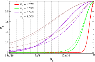
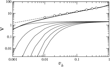
Fig.1 shows the excitation spectrum for different velocities. For a finite chain of sites the lowest energy mode is , this means that, for instance, at the sweep can be considered adiabatic up to . Looking at Fig.1 one can compare the exact result and the Landau-Zener formula that reproduces surprisingly well the exact solution for final field even for rather high . This confirms that the physics of the process is ruled by the Landau-Zener tunneling [17]. One can also observe that for sufficiently low sweeping rate the excitation density just after the transition point () is the same as found at .
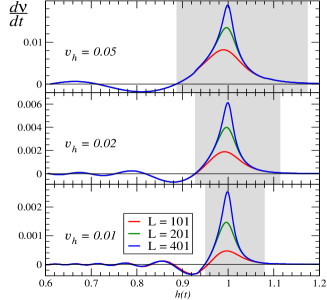
An adiabatic and a sudden region can be distinguished: when the system enters the sudden region the number of excitations rapidly increases up to some maximum value. Afterwards, an oscillatory behavior of the excitation density is observed. Thus, a sensitive (though not unique) possibility to identify the sudden region is the time derivative of the excitation density . Using this method the sudden region can be depicted as the grey shaded regions in Fig.2. At fixed , the number of excitations clearly depends on the density of states (DOS) between the ground state energy and the “sweeping energy” . In particular only few modes contribute to the total excitation density and their number is related to the minimum gap and to the DOS (upper left panel of Fig. 2). When the sweeping velocity increases the sudden region broadens (Fig. 2, right panel). The Kibble-Zurek scenario predict the width of this region to be proportional to the squareroot of the sweeping velocity: .
Already a much less detailed quantity reveals similar insight and admits comparison with reference [8]; namely the total excitation probability
| (9) |
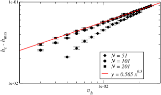
Like , it exhibits a maximum just after the crossing of critical point (see Fig. 3). We define , where is the value of the field where reaches its maximum. The value of evaluated in this way depends on due to the -dependence of the gap. It is only the extrapolation of to that clearly displays the Kibble-Zurek square root behavior as can be seen from the log-log plot in Fig. 3.
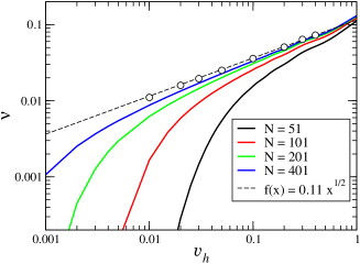
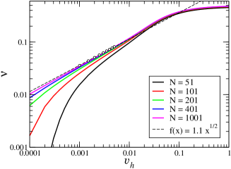
In order to verify the ZDZ scaling law of the excitation density, we plot as function of the sweep velocity in Fig.4. The data extrapolated to the thermodynamic limit agrees well with the expected scaling law independently of . In particular for the Ising model we find , while previous analytical studies based of a LZ [17] and perturbative [13] approximated approaches overestimated it. With decreasing , the minimum gap decreases linearly in while the density of state increases as . The combined effect results in an overall enhancement of the number of excitations in the system and in the thermodynamic limit the density of excitations increases as . This is well verified by comparison of the curves in Fig.4 for (left panel) and (right panel).
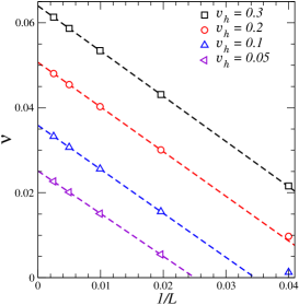
One can wonder whether the ZDZ scaling is a pure many-body effect or determined already by the first excited state alone. In order to answer this question it is important first to observe in Fig.5 the extrapolation of for . The thermodynamic limit is reached with a perfect linear behavior in as expected by the constant value of the DOS at low energy333The DOS in the low energy limit at reads . However, this scaling holds only for large enough values of . To be precise, a sufficiently large number of excited states must be taken into account in order to get the correct thermodynamic limit of .
Even though the first excited state certainly gives the main contribution to the overall excitation density at low sweep velocities, Fig.6 shows that all the levels between the lowest excited state up to the sweeping energy are necessary for the ZDZ scaling to show up. At fixed and in the limit the number of levels in this interval is . So, we conclude the effect to be essentially due to many-body physics rather than to a simple level crossing.
The last important issue of this section is to examine how the mesoscopic (finite) dimension of the spin chain affects the ZDZ scaling behavior and eventually the adiabatic passage through a quantum phase transition. In fact, two competing effects arise when chains of finite length are considered:
-
•
on the one hand, finite means finite gap at and the fidelity of the adiabatic passage is bounded by the ZDZ scaling law;
-
•
on the other hand, finite also implies large mesoscopic fluctuations of the excitation number produced during the sweep, i.e. the average quantities can lose their importance in favor of higher moments.
To address this question, we evaluated the mean square fluctuations of the average density of excitations
| (10) | |||||
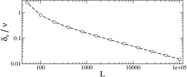
The relative fluctuations are plotted in Fig. 7 for the quantum Ising model, i.e. , and a moderate sweeping velocity. The striking feature that emerges from this analysis is the high sensitivity of the relative fluctuation to the size of the system. Even for rather large lattice size () the relative weight of is as large as 18% and rapidly increase up to 80% for . When the rate of the passage is given, small lattice size implies few excitations on average, but also very large fluctuations in their number and thus a lack of information about the final state.
Let us remark that the ZDZ scaling emerges correctly only in the thermodynamic limit where the relative fluctuations are strongly suppressed. Thus, even if the dynamics of the model (1) is governed by the Landau-Zener tunneling of non-interacting particles, the ZDZ scaling is the proper signature of the quantum critical point crossed during the sweep rather than the result of single particle tunneling processes.
5 Robustness of the adiabatic passage in the presence of noise
A real experimental setup is subject to noise, another source that may corrupt the adiabatic passage fidelity. Here, we examine the case of a noisy driving field, , where is a stochastic field. The simplest choice of a white spectrum for (i.e. and ) will be enough for understanding the main features due to noise and decoherence. The effect of the noise is that a diagonal stochastic term enters the Hamiltonian (2), leading to
| (11) |
In order to study the dynamics of such a system one has to deal with the density matrix formalism and to solve the Lindblad equation [25]
| (12) |
that can be rewritten as
| (13) |
where is the Bloch vector defined by . The Lindbladian here takes the form
| (14) |
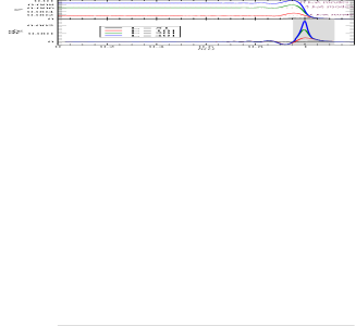
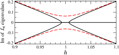
The stochastic noise induces a nonhermitian perturbation to the original Hamiltonian (1). The presence of such kind of perturbations can radically modify the physics of the unperturbed (hermitian) system, in particular when the latter has degeneracy or quasi-degeneracy points, as is the case here: degeneracy or quasi-degeneracy points typically evolve into branch-points of nonhermitian degeneracies [18]. Indeed, two eigenvalues (and the two eigenvectors) of the fermionic system (11) merge in a finite interval of , as compared with a single point without noise. This is seen in Fig. 8 where the imaginary part of eigenvalues of the Lindbladian versus the field are plotted.
Analysis of the noisy case admits to answer two fundamental questions:
-
•
Is it still possible to discriminate the adiabatic from a sudden regime in the presence of noise?
-
•
How robust is the KZ mechanism with respect to noise?
Solving (numerically) Eq. (13) we evaluate the kink density (excitation density) of the system using Eq. (8). It is shown in Fig. 9 for the Ising model () after a sweep of the field from to .
The excitation density of the system increases considerably with the noise strength up to the saturation value (the maximum number of kinks is ). Besides this, there are two new and striking features:
-
1.
the considerable noise instability of the adiabatic approximation even if is orders of magnitude smaller than the excitation gap;
-
2.
the non monotonic behavior of the excitation density with the quench rate .
In order to understand this somehow counterintuitive behavior, all relevant time scales for the adiabatic passage need to be taken into account: the relaxation time , which is the only relevant scale in the noiseless case, and the decoherence time [in the white noise case ]. Both time scales have to be compared with the sweeping time . In order to faithfully drag a quantum state by the drive, the sweeping rate has to be much slower than the gap of the system, , but, on the other hand, it has to be much faster than the dephasing rate, . Then, the condition for the success of the adiabatic passage is that .
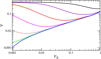
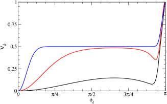
This is nicely seen from the excitation probability as a function of (Fig. 10, left panel) and explains the observed non-monotonicity. The same feature is resolved in terms of modes in the right panel of the same figure. When is of the order of or even larger, most of the modes lose their quantum coherence during the sweep irrespective of the velocity. Eventually, the excitation density of each mode saturates to the value 1/2. The relevance of the appearing of the decoherence time compromises the distinction between the adiabatic and the sudden region.

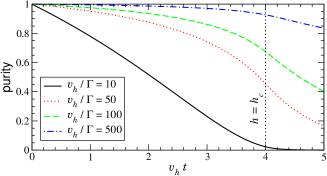
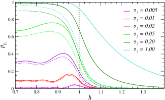
The noise progressively degrades the state of the system into a mixed one. This shows up in Fig.11 looking at the behavior of the purity defined as , that we find to depend solely on the velocity-to-noise ratio . The rate of degradation of the state during the sweep is constant only far from the critical point and this is particularly evident in the case of low velocity-to-noise ratio (full line) where the state mixes up almost completely before reaching . For large enough values of , approaching the critical point the mixing rate of the state increase as shown by the flex-point in the purity close to . This puts clear emphasis on the various facets of noise: besides the mere relaxation-excitation process the main effect consists in decoherence, i.e. mixing of the density matrix. The latter effect has been discarded in a previous work on this subject [19]. We conclude that the (quasi-)degeneracy point not only gives a limit to the rate the parameters of the Hamiltonian may change, but more importantly, it amplifies the effect of decoherence.
6 Conclusions
We have analyzed the dynamical crossing of a quantum phase transition analytically for an ideal clean system and numerically in the presence of white noise. Our focus was to determine the robustness of the adiabatic passage trough a quasi degeneracy point of a many-body system when one considers the effects of finite sweeping period, mesoscopic fluctuations and stochastic forces.
We found a surprisingly high predictive power of the Landau-Zener formula for the final excitation density, when several modes are taken into account. Its validity exceeds significantly the validity range attributed to it in Ref. [17] when the number of Landau-Zener modes to be taken into consideration are determined by the density of states and the characteristic energy scale of the sweep. This number diverges in the thermodynamic limit and it is only in this limit that the ZDZ-scaling [9] manifests. In this sense is this scaling essentially due to collective many-particle physics rather than to the Landau-Zener tunneling of few two-level systems. In addition huge fluctuations around the average excitation density dominate the state during the sweep, in particular for not too large systems. This tells that the physics of the transition is not entirely captured by the excitation average and its square root ZDZ-scaling. The implication of this fact deserve further analysis in order to understand its implications for AQC. In fact, large fluctuations on the average number of excitations implies a loss of information on the final state of an AQC process.
The presence of noise corrupts the success of a possible adiabatic passage for low sweeping velocities due to the opening of a non-hermitian degeneracy leading to a “critical region” rather than just a singular point. The same phenomenon appears also in presence of just an avoided level crossing or a quasi-degeneracy of the spectrum. This leads to an all-over increase of the average excitation density, but it is shown that the most devastating effect of the noise on the transfer fidelity across a non-hermitian degeneracy region is the decay of the state purity that is emphasized by the passage through the degeneracy. Therefore, one has to consider a second time scale besides : the dephasing time. These two time scales are the upper and lower bound for the sweeping rate. Thus there exists an optimal velocity for each noise level that minimizes the fidelity loss.
Finally let us comment on different kind of noise couplings that could be of interest for future studies. In fact, one can wonder how the present conclusions may change if the stochastic variables couple with , breaking the symmetry of the system. Even though the noise coupling we considered preserves the partity symmetry of the Hamiltonian (but not the time reversal one), it causes both relaxation (for ) and decoherence. In this sense, it provides a complete phenomenology. Moreover, the main feature we find, namely the enhancement of the mixing up rate of the state, should be independent on the kind of noise coupling. With this respect, it would be interesting to study colored noise that can strongly modify the dephasing time; it should also have an effect on the white-noise induced increase of the excitation density with time during all the sweep.
Appendix A Exact diagonalization of the XY model in transverse field
In order to diagonalize the one-dimensional XY model in transverse magnetic field (1) we follow Refs. [7, 14, 15] and perform the substitution
| (15) | |||||
| (16) |
The resulting (hard-core bosonic) Hamiltonian becomes
| (17) |
Here we restricted ourselves to an odd number of sites with integer . Though this is not crucial for the exact diagonalization of the Hamiltonian, this becomes equivalent to the restriction to an odd total number of particles – and hence no boundary phase – when starting from a fully polarized state at very large magnetic field.
The Jordan-Wigner transformation
| (18) | |||||
| (19) |
further transmutes the Hamiltonian into fermionic form
| (20) |
Subsequent Fourier transformation
| (21) |
completely decouples the Hamiltonian, so that , where acts in the 4-dimensional Hilbert space . Due to the parity symmetry, it further decouples into . Where , while in the even-occupation Hilbert space and basis one obtains
| (24) | |||||
| (27) | |||||
| (30) |
Expressed in Pauli matrices this is
The eigenvalues and the ground state of the nontrivial second part are given by Eqs.(3) and (4), respectively.
Appendix B Exact time evolution of the XY model in transverse field
The Heisenberg equation (7) for the time evolution operator has been solved in Ref. [7] to obtain the exact time evolution of correlation functions of the model. Using the notation
we obtain the following set of differential equations
| (31) | |||||
| (32) |
¿From these equations and the initial conditions one concludes and and the missing amplitudes are extracted as
| (33) | |||||
| (34) |
The differential equation (31) is exactly solvable if is polynomial in [23] and even for particular cases of transcendental dependence of [7]. For the simplest case , with , the solution is
In our notation is the confluent hypergeometric function and has the series expansion
with the Pochhammer symbol. Its pole structure is that of the gamma function such that with the entire function . The generalized Hermite polynomials are expressed in terms of the confluent hypergeometric function
At integer values of , this function coincides with the Hermite polynomials.
References
- [1] Thouless D J 1983 Phys. Rev. B 27 6083
- [2] Switkes M, Marcus C M, Campman K and Gossard A C 1999 Science 283 1905
- [3] Brouwer P W, 2002 Phys. Rev. B 58 R10135
- [4] Siewert J and Brandes T 2004 Adv. Solid State Phys. 44 181
- [5] Farhi E, Goldstone J, Gutmann S and Sipser M, 2000 Quantum Computation by Adiabatic Evolution Preprint quant-ph/0001106
- [6] Sachdev S 2000 Quantum Phase Transitions, (Cambridge: Cambridge University Press)
- [7] Barouch E, McCoy B M and Dresden M 1970 Phys. Rev. A 2 1075
- [8] Murg V and Cirac J I 2004 Phys. Rev. A 69 042320
- [9] Zurek W H, Dorner U and Zoller P 2005 Phys. Rev. Lett. 95 105701
- [10] Kibble T W B 1976 J. Phys. A 9 1387
- [11] Zurek W H 1985 Nature 317 505
- [12] Zurek W H 1996 Phys. Rep. 276 177
- [13] A. Polkovnikov 2005 Phys. Rev. A 72 161202
- [14] Lieb E, Schultz T, Mattis D 1961 Ann. Phys., NY16 407
- [15] Pfeuty P 1970 Ann. Phys., NY57 79
- [16] E. Barouch and B.M. McCoy 1971 Phys. Rev. A 3 786
- [17] Dziarmaga J 2005 Phys. Rev. Lett. 95 245701
- [18] Berry M V 2004 Czech. J. Phys. 54 1039
- [19] Childs A M, Farhi E, and Preskill J 2002 Phys. Rev. A 65 012322.
- [20] Åberg J, Kult D, and Sjöqvist E 2005 Phys. Rev. A 71 060312(R)
- [21] Roland J and Cerf N J 2005 Phys. Rev. A 71 032330
- [22] Zener C 1932 Proc. Royal Soc. 137 696
- [23] Voros A 1999 J. Phys. A 32 5993 Erratum: ibid. 2000 33 5783.
- [24] Landau L D 1932 Phys. Z. U.S.S.R. 1 426
- [25] Lindblad G 1976 Commun. Math. Phys. 48 119; Gorini V, Kassakowski A, and Sudarshan E. C. G. 1976 J. Math. Phys. 17 821.