Perturbative calculation of non-local corrections to dynamical mean field theory

Abstract

A technique allowing for a perturbative treatment of nonlocal corrections to the single-site dynamical mean-field theory (DMFT) in finite dimensions is developed. It is based on the observation that in the case of strong electron correlation the one-electron Green’s function is strongly spatially damped so that its intersite matrix elements may be considered as small perturbations. Because the non-local corrections are at least quadratic in these matrix elements, DMFT in such cases may be a very accurate approximation in dimensions $d=$ 1–3. This observation provides a rigorous justification for the application of DMFT to physical systems. Furthermore, the technique allows for a systematic evaluation of the nonlocal corrections. This is illustrated with two explicit examples. First we calculate the magnetic short range order parameter for nearest neighbor spins in the insulating phase of the half filled Hubbard model on the square lattice which exhibits an excellent agreement with the results of a recent cluster approach. As a second example we study the lowest order correction to the DMFT self-energy and its influence on the local density of states.

I Introduction

The description of systems of strongly correlated electrons provided by the dynamical mean field theory (DMFT) has significantly improved our understanding of this class of materials.Metzner and Vollhardt (1989); Georges et al. (1996); Held et al. (1997); Imada et al. (1998) The major limitation of DMFT lies in its single-site nature, Georges et al. (1996); Held et al. (1997) which makes it unable to account for spatial correlations in finite-dimensional systems. To remedy this deficiency, cluster generalizations of DMFT have been devised (see discussions on this subject in Refs. Maier et al., 2005 and Okamoto et al., 2003). However, in order to recover the thermodynamic limit, clusters of sufficiently large size should be used.Maier et al. (2005) This strongly enhances the numerical effort needed to solve the corresponding DMFT equations, because the number of quantum variables to be simulated grows proportionally to the number of atoms in the cluster. To alleviate this difficulty, less costly but less accurate numerical approaches have been proposed.García et al. (2004); Dai et al. (2005); Okamoto et al. (2005) In our opinion, this is not a viable solution, because the reduction of errors brought about by the larger number of atoms in the cluster can be overcompensated by the cruder treatment of the quantum effects.

The aim of the present paper is to propose a perturbative approach accounting for nonlocal corrections to DMFT, with the latter being considered as the zeroth order approximation. The approach derives from the general method proposed in Ref. Tokar, 1985. This so-called gamma-expansion method (GEM) proved to be successful, inter alia, in the treatment of the local atomic correlations or short range order in the electronic theory of alloys. Masanskii and Tokar (1988); Boriçi-Kuqo et al. (1998). Here we apply it to the Hubbard model on a square lattice and in the insulating phase, which is well described by the alloy analogy (or Hubbard III approximation) Hubbard (1964); Georges et al. (1996), and therefore should be amenable to the same technique. This will be illustrated below with an explicit calculation of the magnetic short range order (SRO) for this model. The non-local magnetic correlations are of paramount importance for the theories of high temperature superconductivity based on the spin fluctuation mechanism,Scalapino (1995) and their enhancement should therefore be of interest in these theories. In particular, both the Neel and the superconducting transition temperatures should monotonically depend on the strength of the short range magnetic correlations. In this respect the observation made in Ref. Okamoto et al., 2005 that different cluster theories give short range correlations differing roughly by a factor of two provides an additional reason for developing non-cluster based treatments of non-local correlations.

The proposed expansion is based in part on the widely accepted opinion that the single-site DMFT which is exact in infinite dimensions provides us with a picture of the strong correlation phenomena which is qualitatively valid also in physical dimensions $d=$1–3. In other words, it is the single-site dynamics which contain the essence of the problem while intersite correlations play lesser role and so may be considered as correction terms.

An approximate non-local theory in finite dimensions, in which the single-site DMFT is used as the source of information on the local correlations has recently been proposed by KusunoseKusunose (2006) and Toschi et al.Toschi et al. (2007). In essence, the method consists in first finding local irreducible vertex functions from the full DMFT correlators and then using these in the Bethe-SalpeterKusunose (2006) or parquetToschi et al. (2007) equations coupled with Dyson-like equations for the electron self-energy with nonlocal electron propagators in order to find the nonlocal self-energy. From our point of view the main deficiency of such approaches is the lack of consistency: The electron propagators in a skeleton expansion are the same in side-pieces and inside the crosspieces of a ladder diagram. Taking into account that for large values of the coupling constant there is no reasons for the smallness of the terms in the ladder sums, in a strict mathematical sense the series are divergent. So the neglect of non-local contributions in some parts of the diagrams not only is unfounded but may also lead to serious numerical errors. In Ref. Kusunose, 2006 a reference to the spirit of the DMFT in infinite dimensions was invoked where the irreducible vertices inside the ladder series can be chosen to be local without loss of accuracy.Zlatić and Horvatić (1990); Georges et al. (1996) This, however, is completely due to specifics of the $d=\infty$ case, while in finite dimensions the leading nonlocal corrections are are proportional to $O(1/d^{1/2})$Toschi et al. (2007) and thus are quite large in physical dimensions $d=$1–3. In our approach, however, the smallness of the non-local contributions can be explicitely established a priori.

II The model

We are going to study the Hubbard model defined by the Hamiltonian

$$\hat{H}=-\sum_{i,j,s}t_{ij}\hat{c}^{\dagger}_{is}\hat{c}_{js}+U\sum_{i}\hat{n}_{i\uparrow}\hat{n}_{i\downarrow}\equiv H_{0}+H_{U},$$ (1)

where the number operators $\hat{n}_{is}$ for electrons with the spin projection $s=\uparrow,\downarrow$ are expressed through the creation and annihilation operators $\hat{c}^{\dagger}_{is}$ and $\hat{c}_{is}$ as: $\hat{n}_{is}=\hat{c}^{\dagger}_{is}\hat{c}_{is}$; the intersite matrix elements $t_{ij}$ connect nearest neighbor sites and coincide with the hopping integral $t$ and the on-site matrix elements $t_{ii}$ are set equal to the chemical potential $\mu$.

In the functional integral formalism (see, e.g., Ref. Vasiliev, 1998) the generating functional of the Green’s functions is [note the absence of the caret on the Grassmann variables below in contrast to the operators in Eq. (1)]:

$$Z[A,A^{+}]=\int D\psi\exp\left\{-\int_{0}^{\beta}d\tau\left[\sum_{i}\psi_{i}^{+}(\tau)\partial_{\tau}\psi_{i}(\tau)\right.\right.$$ (2)

$$+\left.\left.H(\tau)+\sum_{i}A_{i}^{+}(\tau)\psi_{i}(\tau)+\sum_{i}\psi_{i}^{+}(\tau)A_{i}(\tau)\right]\right\}$$

[cf. Eqs. (29) and (30) of Ref. Georges et al., 1996]. Here the Grassmann variables $A,A^{+}$ are the spinor source fields which are conjugate to the physical spinor fields corresponding to the electrons

$$\psi_{i}(\tau)=\left[\begin{array}[]{c}{c}_{i\uparrow}(\tau)\\ {c}_{i\downarrow}(\tau)\end{array}\right]$$ (3c)

and

$$\psi^{+}_{i}(\tau)=[\bar{c}_{i\uparrow}(\tau),\bar{c}_{i\downarrow}(\tau)],$$ (3d)

where $\tau$ is the thermodynamic imaginary “time”, and $\beta=1/k_{B}T$, where $T$ is the temperature and $k_{B}$ the Boltzmann constant. Here and below we shall omit the constants originating from normalizations of functional integrals, because in the present paper we are interested only in correlation functions. The latter are obtained as functional derivatives of the generating functional (2) at zero value of the functional arguments, divided by $Z[0,0]$, so the normalization is irrelevant.

If the system is in its normal (i. e., non-superconducting) state and, besides, is paramagnetic, (the case we consider in the present paper), the exact one-electron Green’s function $G_{ijs}(\tau-\tau^{{}^{\prime}})$ as well as the self-energy $\Sigma_{ijs}(\tau-\tau^{{}^{\prime}})$ are independent of the spin direction $s=\uparrow,\downarrow$, so we omit this subscript for brevity. $G$ and $\Sigma$ are connected via the usual relation which we symbolically write as

$$G=(\partial_{\tau}+\hat{t}-\Sigma)^{-1}.$$ (4)

The standard diagrammatic analysis (see, e. g., Ref. Vasiliev, 1998) allows one to represent the generating functional of the Green’s functions (2) as:

$$Z[A,A^{+}]=\exp(A^{+}GA)R[GA,A^{+}G].$$ (5)

To simplify notation, here and below the summations over the site and spin indices as well as integrations over the imaginary “time” are implicitly assumed in all products of quantities which depend on those mentioned. $G$ in Eq. (5) is the exact Green’s function defined in Eq. (4). The exponent on the right hand side of Eq. (5) corresponds to the free propagation of electrons while the functional $R$ describes their mutual scattering and, diagrammatically, is represented by the matrix elements of the $S$-matrix with $GA$ “tails” attached.

III The method

As is well known (see review article Georges et al., 1996 and references therein), in the infinite dimensional case the DMFT equations are exact. In finite dimensions DMFT may be viewed as a single-site approximation similar to the correlated effective field theory of ferroelectrics Lines and Glass (1977) or the coherent potential approximation in the theory of disordered alloys.Elliott et al. (1974) The latter approximations were found to be quite successful, so the non-local corrections are expected to be small. In Ref. Tokar, 1985 a method of explicit calculation of these corrections was proposed, based on the observation that in the self-consistent perturbation theory the Feynman diagrams are expressed through the exact correlation function (or propagator) $G$. Thus, if the propagator is such that its on-site (or site-diagonal) matrix element is much larger than its off-diagonal elements, then, firstly, the single-site DMFT-type approximation should be a good one and, secondly, the dominant correction to this approximation can be calculated explicitly by taking into account those off-diagonal matrix elements which are the next largest after the diagonal ones.

It was found that an adequate formalism for the realization of the above intuitive idea is provided by the functional-differential quantum-theoretical formalism.Tokar (1985) In this approach the expression for the generating functional of the $S$-matrix $R$ in Eq. (5) can be cast into the formVasiliev (1998)

$$R[\psi,\psi^{+}]=\exp\left(\frac{\delta}{\delta\psi}{G}\frac{\delta}{\delta\psi^{+}}\right)\exp\left(-\psi^{+}\Sigma\psi-H_{U}\right)$$ (6)

which would coincide with the Hori representationHori (1952) in the case of $\Sigma=0$. In the above formula we have used the freedom in the separation of the total action [the term in the exponent in Eq. (2)] into the “free” (bilinear) part and the interaction part by chosing the (unknown) exact inverse Green’s function $G^{-1}$ as the free part. Then according to Eq. (4) this should be compensated by adding the term $\psi^{+}\Sigma\psi$ to the interaction part $H_{U}$. The validity of the above representation can be easily shown both formallyTokar (1997) and through a diagrammatic analysis.

The equation for the unknown exact one-electron Green’s function can be obtained from its definition via the double functional differentiation of the generating functional (2):

$$G=Z[0,0]^{-1}\delta^{2}\ln Z[A,A^{+}]/\delta A\delta A^{+}|_{A,A^{+}=0}.$$

Substituting here the expression (5) we obtain the following equation:

$$\left.\delta^{2}\ln R[\psi,\psi^{+}]/\delta\psi_{i}(\tau)\delta\psi^{+}_{j}(\tau^{{}^{\prime}})\right|_{\psi,\psi^{+}=0}=0.$$ (7)

III.1 The gamma expansion method (GEM) Tokar (1985)

The last equation is exact and completely general (i. e., independent of any approximation scheme). To solve it in the case of strong correlation (large $U$) we first note that in Ref. Schindlmayr, 2000 it was shown that at finite temperature the one electron Green’s function is exponentially damped at large distances. This confirms the original suggestion of Ref. Tokar, 1985 about the spatial asymptotic behavior of the correlation functions as

$$G_{ij}\propto\exp(-|i-j|/\xi)=O(\gamma^{|i-j|}),$$ (8)

where $\gamma=\exp(-1/\xi)$. Assuming that the correlation length $\xi$ is small, the Feynman diagrams containing large distance Green’s functions can be neglected and the solution can be approximated by the local contribution plus a few terms accounting for correlations with neighboring sites.Tokar (1985)From Eq. (8) it is easy to understand why our approach has DMFT as the zeroth order approximation. DMFT is exact in infinite dimensions because in dimension $d$ the largest off-diagonal matrix elements of the Green function are bounded by a constant of $O(1/d^{1/2})$ and so vanish at $d=\infty$.Metzner and Vollhardt (1989); Georges et al. (1996) The condition (8) with small $\gamma$ presumes that the off-diagonal elements nearly vanish. Thus, DMFT should be a good approximation in such cases in any dimension.

Because the spatial dependence of the self-energy can be expressed through its dependence on the Green’s function, we may assume that both $G$ and $\Sigma$, considered as matrices in the lattice site indices $i,j$, are diagonally dominated, so their separation into diagonal and non-diagonal parts is the separation into the leading contribution and correction terms:

$$G=gI+\tilde{G},$$ (9)

where $I=\delta_{ij}$ and $g\equiv G_{ii}$. Similarly,

$$\Sigma=\sigma I+\tilde{\Sigma}.$$ (10)

It is easy to check that if in the expressions given in the Appendix A one neglects the tilded (i. e., intersite) matrix elements of the Green’s functions and of the self-energy operator, then Eq. (43) substituted into Eq. (7) yields the DMFT equation.Georges et al. (1996)

IV Magnetic short-range order

To illustrate the above general approach we consider the simple problem of the correlation between electron magnetic moments at nearest neighbor (NN) sites on the square lattice at half-filling in the insulating phase.

Following Ref. Okamoto et al., 2005, we measure the magnetic moment in Bohr magnetons so, for example, the local moment at site $i$ is $m^{z}_{i}=n_{i\uparrow}-n_{i\downarrow}=\hat{c}^{\dagger}_{i}\hat{\tau}^{z}\hat{c}_{i}$, where $\hat{\tau}^{z}$ is the Pauli matrix. In the paramagnetic phase, instead of the $\langle m^{z}_{i}m^{z}_{j}\rangle$ correlator used in Ref. Okamoto et al., 2005 we may consider the equivalent correlator

$$\langle m^{-}_{i}(\tau)m^{+}_{j}(0)\rangle=2\langle m^{z}_{i}(\tau)m^{z}_{j}(0)\rangle$$ (11)

which is easier to calculate because it contains only the susceptibility function with opposite spins $\chi_{\uparrow\downarrow}$ while the former correlator requires also the equal spin susceptibility. This is easily seen from the expression

$$m_{i}^{-}=(m_{i}^{+})^{\dagger}=2\hat{c}^{\dagger}_{\uparrow i}\hat{c}_{\downarrow i}$$ (12)

which follows from the usual definition of the Pauli matrices $\hat{\tau}^{\pm}=\hat{\tau}^{x}{\pm}i\hat{\tau}^{y}$.

We define the magnetic short range order (SRO) parameters $\langle m_{i}m_{j}\rangle$ (we omit the superscripts because they can vary in different definitions) as the zero-frequency Fourier component of the correlations functions (11) with $i\not=j$ which is equivalent to their average over the interval $0\leq\tau\leq\beta$. Because the statistical average of the product of the operators (12) contains at least two Green’s functions (see Fig. 1), the lowest order contribution to the SRO parameter is $O(\gamma^{2})$ [see Eq. (8)].

A formal expression for $\langle m_{i}m_{j}\rangle$ can be obtained from Eq. (5) by taking the appropriate fourth order functional derivative with respect to the source variables $A$ and $A^{+}$. The derivative of $R[GA,A^{+}G]$ should further be expanded to second order in $\gamma$. The diagrams containing the contributions up to $O(\gamma^{2})$ are shown in Fig. 1. The first diagram comes from the first factor in Eq. (5) corresponding to the disconnected contributions. The second diagram comes from the zeroth order (DMFT) term of the expansion of $R$ and the last diagram corresponds to the $O(\gamma^{2})$ term in the expansion of $R$ (the two four-point single-site vertices connected by two intersite Green’s function lines). Here it is important to note that the diagrams of Fig. 1 should not be confused with the conventional decomposition of two-particle Green’s functions into ladder-type series with the shaded rectangles being the irreducible four-point vertices as is the case with the diagrams shown in Fig. 8(b) of Ref. Georges et al., 1996. Despite of their formal similarity, the meaning of the diagrams in the two cases is very different. While in the above-mentioned Fig. 8(b) the shaded rectangles in the case of physical dimensionalities would correspond to irreducible vertex functions with their spatial dependence fully taken into account, the shaded elements in our Fig. 1 are full i. e., in general reducible two-particle Green’s functions but with their spatial dependence being only local, i. e., restricted to one site ($k$ or $l$) even in physically relevant finite-dimensional case. The ladder-like structure of the diagrams shown in Fig. 1 is purely accidental and will not persist in higher orders.

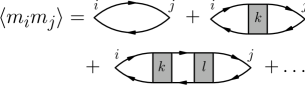
Figure 1: Diagrams contributing into the magnetic short range order to the lowest $O(\gamma^{2})$ order of the small parameter $\gamma$. $i$ and $j$ are two nearest neighbor sites. The arrowed lines correspond to the fully renormalized one-electron Green’s function $G$ and the shadowed rectangles correspond to the fully renormalized amputated single-site vertex $\chi^{a}_{\uparrow\downarrow}$ (see Appendix A for the general definition).

IV.1 The Hubbard III approximation Hubbard (1964)

To explicitly calculate the above diagrams we need expressions for their elements: the Green’s functions and the four-point vertices. As can be seen from Fig. 2, the lowest order non-local correction to the DMFT self-energy $\sigma$ is of order $O(\gamma^{3})$, so in calculations up to $O(\gamma^{2})$ the exact self-energy $\Sigma$ may be approximated by $\sigma$.

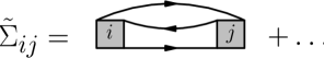
Figure 2: The leading nonlocal correction to the DMFT self-energy. The meaning of the elements of the diagram is the same as in the previous figure.

For the Hubbard model at half-filling in its insulating phase the Fermi liquid properties are not important and the simple Hubbard III approximation can be used.Hubbard (1964) Its detailed discussion, the connection with disordered alloys and the coherent potential approximation (CPA) as well as further references may be found in Refs. Elliott et al., 1974 and Georges et al., 1996. Here we only mention the observation made in the latter reference (see sect. VII.C.2) that the Hubbard III approximation can be obtained as a simple generalization of the atomic case as follows. Let us for generality consider the exact atomic Green function at an arbitrary occupancy $n$Kajueter and Kotliar (1996)

$$g_{at}(i\omega)=\frac{1-n/2}{i\omega+\mu}+\frac{n/2}{i\omega+\mu-U}\equiv D_{at}[i\omega+\mu-\sigma_{at}(i\omega)].$$ (13)

If in this equation we replace the inverse unperturbed atomic Green’s function by its DMFT counterpart as

$$g_{0at}^{-1}(i\omega) \equiv g_{at}^{-1}(i\omega)+\sigma_{at}(i\omega)$$

$$=i\omega+\mu\rightarrow g_{0}^{-1}(i\omega),$$

where, as usual,Georges et al. (1996)

$$g_{0}^{-1}(i\omega)=g^{-1}(i\omega)+\sigma(i\omega),$$ (14)

the Hubbard III approximation

$$g_{s}(i\omega)=\frac{1-n/2}{g_{0}^{-1}(i\omega)}+\frac{n/2}{g_{0}^{-1}(i\omega)-U}$$ (15)

is obtained.

Because the Mott transition takes place only at half-filling corresponding to $n=1$, the insulating Hubbard III solution is valid only in this case. Furthermore, because at half filling the system is explicitly particle-hole symmetric, it is convenient to switch to an explicitly particle-hole symmetric formalism. This is achieved through the replacement (see Ref. Georges et al., 1996 Ch. VII B)

$$g_{0}^{-1}\to g_{0}^{-1}+U/2.$$

In this case Eq. (15) takes a symmetric form which we will use in the rest of the paper

$$g_{s}(i\omega) = \frac{1/2}{g_{0}^{-1}(i\omega)+U/2}+\frac{1/2}{g_{0}^{-1}(i\omega)-U/2}$$ (16)

$$\equiv (1/2)g_{s,s}(i\omega)+(1/2)g_{s,-s}(i\omega).$$

Here, in the second line, we have introduced the partial single-site Green’s functions corresponding to the propagation of electrons with their spins parallel or opposite to the dominant spin on the site under consideration (see Ref. Elliott et al., 1974). These Green’s functions will be necessary in the next subsection.

Eq. (14) changes to

$$g_{0}^{-1}(i\omega)=g^{-1}(i\omega)-U/2+\sigma(i\omega).$$ (17)

Eqs. (16) and (17) constitute a set to find $g(i\omega)$ and $\sigma(i\omega)$, provided the bare single site Green’s function is known.Georges et al. (1996) The latter is given by the site-diagonal matrix elements of the lattice Green’s function and is usually calculated as a sum over quasimomenta, which coïncides with the Watson integral in the continuum limitTokar (1985):

$$D(i\omega)=\frac{1}{N}\sum_{\bf k}\frac{1}{i\omega-\epsilon({\bf k})},$$ (18)

where $\epsilon({\bf k})$ is the lattice Fourier transform of the matrix $-{t}_{ij}$ with $\mu=0$. With the use of this function the DMFT Green’s function is obtained as $g(i\omega)=D[i\omega+\mu-\sigma(i\omega)]$.Georges et al. (1996)

Similarly, the matrix element $G_{1}$ of the one-electron Green’s function connecting NN sites can be calculated as $G_{1}=D_{1}[i\omega+\mu-\sigma(i\omega)]$, where, for isotropic matrices ${t}_{ij}$ connecting only NN sites:

$$D_{1}(i\omega)=[1-i\omega D(i\omega)]/qt,$$ (19)

and $q$ is the coordination number ($q=4$ for the square lattice).

We found it convenient to chose among various forms of the Hubbard III (or CPA) equationsElliott et al. (1974) the following one:

$$\sigma(i\omega)=Un/2+(U/2)^{2}g_{0}(i\omega).$$ (20)

At weak coupling, when the first (Hartree) term in Eq. (20) dominates, the DMFT approaches the perturbative solution.

The solution for $n=1$ was obtained by iterating Eq. (20) together with Eq. (17), and is shown in Fig. 3 for a particular set of parameters. As we see, the imaginary part of $i\omega_{n}-\sigma(i\omega_{n})$ is quite large, so the damping with distance of $G_{ij}$ in Eq. (8) is strong Schindlmayr (2000), hence $\gamma$ is really a small quantity.

Figure 3: The DMFT self-energy calculated in the Hubbard III approximation (present work) compared to the quantum Monte Carlo (QMC) simulations of Ref. Okamoto et al., 2005 [$\omega_{n}=\pi k_{B}T(2n+1)$ is the Matsubara frequency].

For example, with the parameters given in Fig. 3

$$\max|G_{1}(i\omega_{n})|\approx 2.5\cdot 10^{-3}t^{-1},$$ (21)

the correction terms being at least of the second order in ${G}_{1}$. This means that in the case under consideration DMFT is a very good approximation.

In the next section we will see that in the case of strong correlation near half filling there exists a mechanism of enhancement of the loop diagrams at low temperatures. At such temperatures the $O(\gamma^{3})$ non-local corrections corresponding to the diagram in Fig. 2 need to be taken into account. We will return to this question after explaining the mechanism of the enhancement.

IV.2 The Curie behavior of the magnetic SRO at low temperatures

From Eq. (21) it follows that deviations from DMFT are small unless there exists some mechanism of enhancement of the correction terms. In this subsection we are going to show that in the half filled strongly correlated Hubbard model such a mechanism does exist and is connected with a peculiar time dependence of the four-point vertex functions entering the diagrams in Fig. 1. The term exhibiting this dependence is the first one in the expression for the atomic vertex function Eq. (B) and, at low temperature

$$\chi^{c}_{\uparrow\downarrow}(i\omega_{1},i\omega_{2},i\omega_{3},i\omega_{4})\approx$$ (22)

$$\approx\frac{1}{2}\delta_{\omega_{1}\omega_{4}}\delta_{\omega_{2}\omega_{3}}\Delta g(i\omega_{3})\Delta g(i\omega_{4}),$$

where the superscript ‘$c$’ stands for ‘connected’, and

$$\Delta g(i\omega)=g_{s,s}(i\omega)-g_{s,-s}(i\omega)=-Ug_{0}(i\omega)g(i\omega).$$ (23)

All other contributions to $\chi^{c}_{\uparrow\downarrow}$ do not lead to an enhancement and can therefore safely be neglected. By analogy with Eqs. (13)—(16) above we may generalize the expression for the vertex function from the atomic to the band case as in the derivation of the Hubbard III approximation in the previous subsection, i. e., by replacing the atomic versions of $g_{s,\pm s}$ by their band counterparts. This can be justified more rigorously by a calculation of the vertex function in the Hubbard III approximation.Tokar (1989)

As was pointed out in Ref. Sarker, 1988, the singular character of the four-point vertex function is most transparent when written in the form of its contribution to the effective interaction functional (A):

$$\frac{1}{2}\sum_{\omega}c^{+}_{\uparrow}(\omega)\phi(i\omega)c_{\downarrow}(\omega)\sum_{\omega^{{}^{\prime}}}c^{+}_{\downarrow}(\omega^{{}^{\prime}})\phi(i\omega^{{}^{\prime}})c_{\uparrow}(\omega^{{}^{\prime}}),$$ (24)

where, according to Eqs. (22), (23), and (A)

$$\phi(i\omega)=Ug_{0}(i\omega)/g(i\omega)$$ (25)

[$g^{-1}$ appears due to the four amputations in Eq. (A)]. It is easy to see that the above vertex function is a product of two independent bilinear terms with the symmetry of the $S^{-}$ and $S^{+}$ spin operators. When transformed to the (imaginary) time the interaction (24) takes the form

$$\frac{1}{2}\int d\tau S^{-}(\tau)\int d\tau^{{}^{\prime}}S^{+}(\tau^{{}^{\prime}}),$$ (26)

where the spin variables are the Fourier transforms of the two factors in Eq. (24). Obviously, the above interaction can be exactly decoupled with the use of the Hubbard-Stratonovich transformation with a time-independent ordinary (i. e., non-functional) variable. This observation provides a rigorous justification of the theories based on the static approximation.Hubbard (1979); Hasegawa (1980); Moriya (1985) We stress that, while in the theories of Refs. Hubbard, 1979; Hasegawa, 1980; Moriya, 1985 the static approximation was introduced through an ad hoc modification of the initial Hamiltonian, in the present approach it was obtained as an approximate (Hubbard III) solution to the Hubbard model, based on the observation made in Ref. Georges et al., 1996 that, in the case of strong coupling and half filling, it accurately reproduces the results obtained in a full-fledged DMFT treatment. In particular, our “by analogy” derivation of the vertex function can be confirmed by the observation that the on-site spin-spin correlation function “develops long-term memory signalling the formation of a local moment” made on the basis of numerical simulations [see Ch. VII.G.1 of Ref. Georges et al., 1996 and Eq. (52) in Appendix B of the present paper].

Thus, because the static field has a zero-frequency Fourier transform we see that at strong coupling the half-filled Hubbard model develops a zero-energy scale. Below we will show that because of this the susceptibility may develop a Curie-like behavior on an energy scale much smaller than the electron bandwidth. The temperature dependence $\sim 1/T$ will enhance the contribution of the corresponding diagram at low temperature,—thus providing a mechanism for the enhancement of the small $O(\gamma^{2})$ contributions mentioned above.

Formally this can be shown as follows. First, to the order $O(\gamma^{2})$ we may neglect the difference between $V$ and $\bar{V}$ in Eq. (41) because according to Eq. (42) their difference depends on the $O(\gamma^{3})$ quantity $\tilde{\Sigma}$. Thus, the $O(\gamma^{2})$ contribution to $R$ in the spin fluctuation channel is obtained from Eq. (41) as the $O(\tilde{G}^{2})$ term in the expansion of the first exponential. The contribution (24) to $V$ will then lead to the the following form for the dominant term in $R$

$$\delta R=\frac{1}{2}\alpha(T)\sum_{j\omega}c^{+}_{j\uparrow}(\omega)\phi(i\omega)c_{j\downarrow}(\omega)\sum_{k\omega^{{}^{\prime}}}c^{+}_{k\downarrow}(\omega^{{}^{\prime}})\phi(i\omega^{{}^{\prime}})c_{k\uparrow}(\omega^{{}^{\prime}}),$$ (27)

where $j$ and $k$ denote nearest neighbor sites and

$$\alpha(T)=-U^{2}\sum_{\omega}[G_{1}(i\omega)g_{0}(i\omega)/g(i\omega)]^{2}.$$ (28)

Here the minus sign appears because of the closed Fermion line made by the two nearest neighbor Green’s functions $G_{1}$. The remaining factors come from the product of two effective interactions $\phi(i\omega)$. We note that the summation over the Matsubara frequencies in Eq. (28) is not supplemented by a $\beta^{-1}$ factor (this will be explained in more detail below). Thus, because the $i\omega$-dependent summand consists of smooth functions and the number of the Matsubara frequencies $\omega_{n}$ scales as the inverse temperature, as the temperature is lowered the sum will diverge as $1/T$. The importance of this observation lies in the fact that this term leads to the magnetic susceptibility satisfying the Curie law which we are going to show with explicit calculations below.

Among the diagrams of Fig. 1 it is the third one which exhibits the Curie behavior. This can be seen as follows. Because our magnetization operators Eq. (12) are dimensionless, their correlator (11) or (IV.2) also has no dimension. The elements of the diagrams in Fig. 1, on the other hand, when Fourier transformed with respect to the imaginary time variables have the following dimensionalities in units of energy:

$$[G]=-1\qquad\mbox{and}\qquad[\chi^{a}_{\uparrow\downarrow}]=[\chi^{c}_{\uparrow\downarrow}][G]^{-4}=2$$ (29)

[see Eq. (B)]. Thus, in the first diagram in Fig. 1 these elements contribute the factor $GG$ which has dimension -2. Because the contribution should be dimensionless, this means that the diagram additionally contains the compensating factor $(k_{B}T)^{2}$ with the dimension 2. According to the diagrammatic rules corresponding to the vertex function (24), in the particle-hole channel the number of summation over the internal variables of a diagram is equal to the number of loops in this diagram. The summation over the Matsubara frequencies scales as $\sim 1/T$ for each loop as explained above. Thus, in the case of the first diagram we have one loop summation of $O(1/T)$ and the factor $O(T^{2})$ so the result is bounded as $T\to 0$. The second diagram has the combination $GG\chi^{a}GG$ of dimension -2, hence the same $O(T^{2})$ additional factor but this time two loop summations bringing the $O(1/T^{2})$ behavior making the diagram to be of order unity. Finally, a similar analysis in the case of the last diagram in Fig. 1 shows that it behaves as $O(1/T)$ because of its three summations over the loop variables. It is this latter diagram which are going to compute explicitly below while neglecting the other two because of their smallness.

The contribution corresponding to this diagram is

$$\langle m^{-}_{i}m^{+}_{j}\rangle\equiv\beta^{-1}\int_{0}^{\beta}d\tau\langle m^{-}_{i}(\tau)m^{+}_{j}(0)\rangle$$

$$=m_{i}m_{j}\alpha(T),$$ (30)

where the on-site magnetizations are

$$m_{i(j)}=-\beta^{-1}\sum_{\omega}\Delta g(i\omega)=U\beta^{-1}\sum_{\omega}g(i\omega)g_{0}(i\omega).$$ (31)

To understand the origin of the contributions to Eq. (IV.2) we first note that the two lines connecting sites $k$ and $l$ on the diagram come from the intersite correction to the four-point vertex in Eq. (41) where to the order $O(\gamma^{2})$ we may restrict $\tilde{G}$ to the NN sites. This explains the appearance of $G_{1}^{2}$ in Eq. (28). Thus, the smallness of the diagram in Fig. 2 is already exhausted by this contribution, so the leftmost and the rightmost propagators may be restricted to on-site Green’s functions $g$. In other words, to the order $O(\gamma^{2})$ we have $i=k$ and $j=l$. The factors $g^{2}$ at sites $i$ and $j$ multiply the two external legs of the vertex (22) which, combined with Eq. (25), leads to expressions of the type of Eq. (23). The summation over frequencies then yields the two factors of the type of Eq. (31). The on-site magnetizations $m_{i(j)}$ (31) calculated with the parameters of Fig. 3 are practically saturated to their maximum value 1 (in Bohr magnetons).

In the two internal lines the amputation factors are not compensated by the propagators because they are now intersite ones ($G_{1}$), so the two vertices (24) introduce the two factors $Ug_{0}/g$. The coefficient $(1/2)\times(1/2)$ coming from the product of two vertices (24) is compensated by the coefficient $2\times 2$ coming from Eq. (12).

The magnetic SRO calculated according to the above formula shows excellent agreement with the cluster calculations of Ref. Okamoto et al., 2005 (see Fig. 4). Because our technique works directly with the thermodynamic limit, this agreement confirms the conclusion of the above reference that their fictive impurity (FI) method is a more reliable cluster approximation than the dynamical cluster approximation which yields a SRO parameter approximately two time larger than in Fig. 4 (see Fig. 14 in Ref. Okamoto et al., 2005).

Because of the $O(1/T)$ enhancement, our perturbative technique becomes less reliable at very low temperature, where a resummation technique should be used. For example, by extending the ladder sum to infinity with the intermediate Green’s functions restricted to $G_{1}$ as above, we would have obtained the usual mean field value for the Neel temperature $T_{N}=qJ$. The value of $T_{N}$ calculated in this way would match that shown in Fig. 10 of Ref. Okamoto et al., 2005. Such an approach, however, is not in the spirit of the GEM. In fact, within the GEM the phase transition temperatures can usually be calculated with much better accuracy than in the mean field approximation. For example, according to Eq. (13) of Ref. Tokar, 1985 the value of $qJ/T_{N}$ in the zeroth order approximation of GEM is given by the Watson integral for the corresponding lattice. In a 2-dimensional system this integral would diverge (see, e. g., Ref. Katsura and Inawashiro, 1971),—thus giving the correct value $T_{N}=0$ in this case. The possibility to develop such an approach for phase transitions in the Hubbard model is currently being investigated.

Figure 4: Magnetic short range order parameter for the NN sites $i$ and $j$ calculated to the lowest nontrivial order of the gamma expansion method (GEM) in comparison with the cluster technique of Ref. Okamoto et al., 2003 [called by the authors the fictive impurity (FI) method] and with the leading term of the high temperature expansion of the superexchange interaction.Anderson (1959); Okamoto et al. (2005) The square dots correspond to data calculated by two different methods in Ref. Okamoto et al., 2005.

A Curie-like behavior is characteristic for localized spins but is difficult to understand in the case of itinerant spins of band electrons.Fazekas (1999) The latter situation may be described by the Hubbard model in the weak coupling limit $U\to 0$. Because in this case conventional perturbation theory applies, all calculations can be done in the finite bandwidth case. But it is more instructive to see how the perturbative limit is attained in the formalism of the GEM. To this end we first note that the approximation (22) is not appropriate in the weak coupling case because it is of second order in $U$. Going back to the defining equation (B), we find that the first order term has the small-$U$ limit

$$\chi^{a}_{\uparrow\downarrow}(i\omega_{1},i\omega_{2},i\omega_{3},i\omega_{4})|_{U\to 0}\approx\delta_{\omega_{1}+\omega_{2},\omega_{3}+\omega_{4}}k_{B}TU,$$ (32)

where we presented the amputated version of the connected correlator because in this case the atomic correlator is the same as in the band case. As we see, now the vertex functions in the diagrams of Fig. 1 contain an additional factor $T$, so that the mechanism of the low-temperature enhancement leading to the Curie law is not operative any more. Because of this and because of the smallness of $U$ it is the first diagram in Fig. 1 which is the main contribution with the second diagram giving the first order correction. Because the first order Hartree term in the Green functions is exact and the vertex in Eq. (32) is also exact, the spin susceptibility calculated within the GEM will be accurate to first order in $U$ at weak coupling.

IV.3 Non-local corrections to the self-energy

The mechanism at the origin of the enhancement in the loop summations in the half-filled Hubbard model will also be operative in the diagram for the lowest-order non-local correction to the self-energy shown in Fig. 2. Indeed, it is easy to see that (i) the contribution to $\tilde{\Sigma}$ coming from the term (27) can be obtained by simply contracting $c_{is}$ and $c^{+}_{js}$ at nearest neighbor sites and (ii) by noting that the contribution thus obtained should be multiplied by 3/2 because the term (27) coming from the product (26) constitutes only 2/3 of the full scalar product $\vec{S}\cdot\vec{S}=S^{-}S^{+}+S^{z}S^{z}$ constituting the full rotationally invariant singular interaction Sarker (1988) leading to the first term in Eq. (B). Thus

$$\Sigma_{1}(i\omega)=\frac{3}{4}[Ug_{0}(i\omega)/g(i\omega)]^{2}\alpha(T)G_{1}(i\omega).$$ (33)

In connection with this expression some comments are in order. From Eq. (28) it follows that the nonlocal self-energy in Eq. (33) is of fourth order in $U$ . Such a term was shown to be the lowest order (in $U$) non-local contribution to the self-energy in the Falicov-Kimball (F-K) model in Ref. Schiller and Ingersent, 1995. Our approximation (22) essentially describes this case because it is based on the local (atomic) approximation to the band electrons—a feature shared by the $f$-electrons in the F-K model.Freericks and Zlatić (2003) In the Hubbard model, the last, linear in $U$ term in Eq. (B), dominates in the weak coupling limit. Its insertion into the diagram of Fig. 2 gives the conventional second order contribution into $\Sigma$.

IV.4 Herglotz properties of spectral functions

Our next comment concerns the fundamental requirement that the imaginary part of the self-energy be negative semi-definite in order to guarantee the positivity of the density of states

$$\rho(E,{\bf k})\equiv-\frac{1}{\pi}{\Im\Sigma(E,{\bf k})}{|G(E,{\bf k})|^{2}}$$ (34)

of the quasiparticles with quasimomentum ${\bf k}$ and energy $E$. The quantities in the right hand side of this equation should be obtained by analytic continuation from the discrete Matsubara frequencies in the upper part of the complex energy plane $z$ to the real axis $E$ as

$$z=\left.E+i\epsilon\right|_{\epsilon\to 0}.$$

This continuation is in general a non-trivial procedure because the quantities to be continued are usually known only in the form of the data of quantum Monte Carlo simulations. Continuation of such data to the real axis is an ill-posed problem the discussion of which as well as the pertinent bibliography may be found in Ref. Georges et al., 1996. We only would like to add that the continuation of a perturbation expansion (like GEM) poses additional problems which are explained in Appendix C.

Because of the simplicity of the Hubbard III approximation, however, it is possible to perform the above analytic continuation explicitly. This will be done below to illustrate the Herglotz properties of the self-energy and the total density of states with the correction term given by Eq. (33). To this end we first derive the expression for the corrected on-site Green’s function. For a hopping matrix connecting only nearest-neighbor sites, we get from Eqs. (4) and (18)]

$$g(i\omega)\equiv G_{ii}(i\omega)=\frac{1}{1-\Sigma_{1}(i\omega)/t}D\left(\frac{i\omega-\sigma(i\omega)+\mu}{1-\Sigma_{1}(i\omega)/t}\right).$$ (35)

From this expression it is easy to see that irrespective of the precise form of the correction term, the total density of states (DOS)

$$\left.\rho(E)=-\frac{1}{\pi}\Im g(z=E+i\epsilon)\right|_{\epsilon\to 0}.$$ (36)

is conserved because the asymptotics of $g(z)$ at large $z$ are the same as those of $D(z)$: $\sim 1/z$ (see Appendix C for further details). However, from the point of view of GEM, Eq. (35) is valid only to lowest order in $\Sigma_{1}$. So it is more prudent (and also more convenient for further analysis) to separate different contributions as

$$g(i\omega) \approx D\left[i\omega-\sigma(i\omega)+\mu\right]$$ (37)

$$+ [\Sigma_{1}(i\omega)/t]\left[D(z)+zD^{\prime}(z)\right]_{z=i\omega-\sigma(i\omega)+\mu},$$

where the second line represents the lowest order correction to DMFT (the first line).

Eqs. (20), (33), (35), and (37) were continued to the real axis and solved with the model parameters used in the calculations above. The results did not show any violation of the Herglotz properties. Therefore, to study the anomalies discussed in Appendix C, a smaller value of $U=3.2t$ was chosen, which corresponds to 80% of the critical value $U_{M}\approx 4t$ for the Mott transition in the Hubbard III approximation, and leads to a more than 30 times larger NN matrix element (21) .

Before proceeding with explicit calculations we would like to remind that our approach is based on the asymptotic behavior of the imaginary-time Green’s functions at finite temperature. The spatial attenuation (8) is defined by the Green’s function behavior at the discrete imaginary energies (the Matsubara frequencies), being more efficient at larger temperatures.Schindlmayr (2000) Therefore, there is no guarantee that the correction terms will remain small when continued to the real energy axis. Explicit calculations below, however, show that the GEM corrections remain generally small even on the real axis.

The GEM-corrected self-energy in energy and wave vector space can be written as [cf. Eq. (10)]

$$\Sigma(z,{\bf k})\approx\sigma(z)+2(\cos k_{x}+\cos k_{y})\alpha\Sigma_{1}^{\prime}(z),$$ (38)

where the prime means that the self-energy (33) has been divided by the SRO parameter $\alpha(T)$, which is the natural expansion parameter in the present case. Since $\alpha(T)$ is negative, Eq. (55) takes the form

$$|\alpha|>\left[\max_{\Im\Sigma_{1}^{\prime}(E,{\bf k})>0}\frac{2(\cos k_{x}+\cos k_{y})\Sigma_{1}^{\prime}(E)}{\sigma(E)}\right]^{-1}.$$ (39)

An explicit calculation shows that for the case under consideration the imaginary part of $\Sigma(z,{\bf k})$ is non-negative only when $\alpha>-0.45$. We do not consider this restriction as a severe limitation of the GEM because, in such a situation, the spins in the system are spatially so strongly correlated, that the behavior of the electrons changes qualitatively and more sophisticated techniques should be developed for calculating the Green’s functions (see, e. g., Ref. Sadovskii et al., 2005).

The results of our calculations are shown in Fig. 5. The Hubbard sub-bands at $U=\pm 0.4U_{M}$ are not yet separated. From the shape of the derivative of the DOS with respect to the SRO parameter (lower panel), we expect a transfer of spectral weight from the sides of the subbands to their centers as the temperature is lowered and $\alpha(T)$ becomes more negative. The physics of this transfer is the same as in the Falicov-Kimball (F-K) model of Ref. Hettler et al., 2000. When the local order grows, the atoms became increasingly surrounded by sites with essentially different on-site potentials. In the F-K case these are the atoms filled by the $f$-electrons while in the Hubbard case the surrounding atoms host the electrons of opposite spins. This hampers intersite atomic hopping and causes the subband narrowing. In the F-K model case this can be seen from Fig. 7 of Ref. Hettler et al., 2000. The qualitative difference with our Fig. 5 is only due to (i) the narrow features at the centers of the subbands because of the atomic-like spectrum of the $f$-electrons which are absent in the Hubbard model and (ii) stronger temperature dependence of DOS near the middle of the band because in the 2D F-K model a charge transfer gap opens in the the spectrum at finite temperature. This phase transition at finite temperature is possible because the order parameter of the charge density wave is Ising-like, while in the 2D Hubbard model the ordering is forbidden due to the continuous (rotational) symmetry of the spin variables.

Figure 5: Upper panel: Density of states (DOS) of the half-filled Hubbard model on the square lattice with $U=3.2t$ calculated for two values of the magnetic short range order parameter $\alpha$. The latter was calculated with the use of Eq. (28) for the two temperature shown in the figure. The DOS was calculated via the first order expansion Eq. (37). Lower panel derivative of the DOS with respect to the short range order parameter. All quantities are measured in energy or inverse energy units, with the the hopping parameter $t$ set equal to unity.

Finally, it is worthwhile to note that the enhancement of the intersite correlations discussed in this work for “normal” contractions also takes place for the anomalous means $\langle c_{i}c_{j}\rangle$,Tokar (1989) in which case it leads to a BCS-type superconducting gap equation with the antiferromagnetic intersite correlations playing the role of the pairing interaction (see the review paper Ref. Scalapino, 1995). This problem will be considered in more detail in a future publication.

V Conclusion

As our elementary calculations show, in some cases the GEM allows for a reliable calculation of non-local corrections to DMFT. In the case of the Hubbard model at half filling the corrections are strongly enhanced by spin fluctuations. We expect that a similar (though presumably weaker) enhancement will also take place in the case of small doping. Furthermore, from the discussion above, it is seen that the enhancement occurs in the leading non-local correction to the four-point vertex (last diagram in Fig. 1) and to the self-energy (particle-hole loops in Fig. 2). In both cases the enhancement may be of considerable importance for the spin fluctuation mechanisms of superconductivity formulated either via the Bethe-Salpeter equation for the bound states of the pairs or the BCS equation for the self-energy.Bulut et al. (1993); Scalapino (1995); Maier et al. (2006) This would require more accurate calculation of the four-point vertices with proper account of the Fermi liquid properties. This problem is currently being investigated in the framework of the approaches of Refs. Hirsch and Fye, 1986; Georges et al., 1996; Rubtsov et al., 2005, and Werner et al., 2005.

Appendix A Renormalized vertices

The relationship between the conventional path integral representation of partition functions and the Hori functional-differential representation can be formally established by first using the Gaussian functional integration formula to decouple the second order functional derivative into a first order derivative multiplied by a Grassmann field (say, $\eta$) in a way completely analogous to the Hubbard-Stratonovich transformation and then applying the formula for the functional shift (Ref. Vasiliev, 1998, Ch. 1),

$$\exp(\eta\delta/\delta\psi)f[\psi]=f[\psi+\eta]$$ (40)

valid for any functional $f$ (and similarly for $\eta^{+},\psi^{+}$). Next with the sequence of transformations explained in Refs. Tokar, 1985 and Tokar, 1989 one obtains:

$$R[\psi,\psi^{+}]=\exp\left(\frac{\delta}{\delta\psi}\tilde{G}\frac{\delta}{\delta\psi^{+}}\right)\exp\left(\psi^{+}\hat{g}^{-1}\psi-\bar{V}[\psi,\psi^{+}]\right),$$ (41)

$$e^{-\bar{V}[\psi,\psi^{+}]}=\exp\left(-\frac{\delta}{\delta\psi}\hat{g}\tilde{\Sigma}\hat{g}\frac{\delta}{\delta\psi^{+}}\right)\exp\left(-\sum_{i}V[\psi_{i},\psi^{+}_{i}]\right),$$ (42)

$$V[\psi_{i},\psi^{+}_{i}] = -\ln\left(\int D\eta D\eta^{+}\exp\left\{-\psi^{+}_{i}\hat{g}^{-1}\eta-\eta^{+}\hat{g}^{-1}\psi_{i}\right.\right.$$ (43)

$$+\left.\left.\eta^{+}(\hat{g}^{-1}+\hat{\sigma})\eta-H_{I}[\eta,\eta^{+}]\right\}\vphantom{\int}\right),$$

where

$$H_{I}[\eta,\eta^{+}]=\frac{U}{2}\int_{0}^{\beta}d\tau(\eta^{+}\cdot\eta)^{2},$$ (44)

and the spinors $\eta$ and $\eta^{+}$ have the structure of Eqs. (3c) and (3d)

$$\eta(\tau)=\left[\begin{array}[]{c}{a}_{\uparrow}(\tau)\\ {a}_{\downarrow}(\tau)\end{array}\right]$$ (45c)

and

$$\eta^{+}(\tau)=[\bar{a}_{\uparrow}(\tau),\bar{a}_{\downarrow}(\tau)].$$ (45d)

In Eqs. (41) and (42) the summation over the site indices and the integration over the thermodynamic “time” $\tau$ is implicitly assumed in all products of fields and matrices. In Eqs. (43)–(45d) $\eta$ is not supplied with the site index because we consider the normal, paramagnetic, and translationally invariant case in which all sites are equivalent. In this case the matrices $\hat{g}$ and $\hat{\sigma}$ are diagonal and proportional to the unit matrix because $g_{\uparrow}=g_{\downarrow}=g$ and similarly for the self-energy. The formalism, however, can be easily generalized to a general broken symmetry case which would essentially amount to introducing site-dependent field $\eta$ and the the Green’s function and self-energy matrices of general form.Tokar (1985, 1989)

Thus, according to Eq. (43) the effective on-site interaction vertices are given by

$$V[\psi_{i},\psi_{i}^{+}]=\sum_{\mbox{even $n>2$}}\int_{\tau_{1}}\int_{\tau_{2}}\dots\int_{\tau_{n-1}}\int_{\tau_{n}}$$

$$\psi_{i}^{+}(\tau_{1})\psi_{i}^{+}(\tau_{2})\dots\chi_{n}^{a}(\tau_{1},\tau_{2},\dots,\tau_{n-1},\tau_{n})\dots\psi_{i}(\tau_{n-1})\psi_{i}(\tau_{n}),$$ (46)

where the “amputated” vertex is defined by

$$\chi_{n}^{a}(\tau_{1},\tau_{2},\dots,\tau_{n-1},\tau_{n})=\int_{\tau^{\prime}_{1}}\int_{\tau^{\prime}_{2}}\dots\int_{\tau^{\prime}_{n-1}}\int_{\tau^{\prime}_{n}}\hat{g}^{-1}(\tau_{1}-\tau^{\prime}_{1})\hat{g}^{-1}(\tau_{2}-\tau^{\prime}_{2})\dots$$

$$\langle\eta(\tau^{\prime}_{1})\eta({\tau^{\prime}_{2}})\dots\eta^{+}(\tau^{\prime}_{n-1})\eta^{+}(\tau^{\prime}_{n})\rangle^{c}_{S_{eff}}\dots\hat{g}^{-1}(\tau^{\prime}_{n-1}-\tau_{n-1})\hat{g}^{-1}(\tau^{\prime}_{n}-\tau_{n}).$$ (47)

The summation in Eq. (A) is restricted to the values of $n>2$ because according to the zeroth order of GEM (or DMFT—see below) approximation Eq. (7) with $i=j$ the term $n=2$ turns to zero, so $V[\psi_{i},\psi_{i}^{+}]$ contains only true many-electron interactions. The angular brackets in Eq. (A) denote the statistical averaging in Eq. (43) with the effective actionGeorges et al. (1996)

$$S_{eff}=\eta^{+}(\hat{g}^{-1}+\hat{\sigma})\eta-H_{I}[\eta,\eta^{+}]$$ (48)

with the superscript ‘$c$’ meaning that only the connected diagrams should be kept. It should be noted that because $\psi_{i}$ and $\eta$ in the above equations are of the spinor type, the vertices $\chi_{n}^{a}$ are tensor quantities possessing in general $2^{2n}$ components. In the symmetric case under consideration many of the components are equal zero and many among them are mutually equal. For example, the $n=2$ four-point function is fully defined by two scalar vertices: $\chi^{a}_{\uparrow\downarrow}$ and $\chi^{a}_{\uparrow\uparrow}$ of which in our calculation of the spin correlation function only the first one is needed.

Thus, the effective single site vertices in Eq. (A) are the connected [because of the logarithm in Eq. (43)] amputated [because of the $\hat{g}^{-1}$ factors in Eq. (A)] single-site correlation functions calculated with the effective action given by Eq. (48). In Eqs. (43), (44), (A), and (A) all fields and matrices are assumed to be single-site. To simplify notation the site dependence has been omitted. It can be easily restored by supplying all quantities in these formulas with the subscript $i$.

There is an infinite number of spatially local interactions in the GEM but, in contrast to what happens in conventional perturbation theory, the smallness is provided by the off-diagonal (in the lattice site indices) elements of the propagator $\tilde{G}$ and of the self-energy $\tilde{\Sigma}$ [see Eqs. (41), (42), and (43) above]. So the order of a correction will be classified by the number and length of the propagators in the corresponding diagram.Tokar (1985) For example, if Eq. (7) is restricted to a single site, i. e., if we assume that $i=j$, then Eqs. (43), (44) with all tilded quantities set to zero together with Eq. (7) will reproduce the DMFT theory of Ref. Georges et al., 1996. Because $i=j$ means the zeroth order of the GEM [see Eq. (8)] the above means that DMFT is equivalent to the zeroth order of the GEM.

Appendix B Atomic four-point correlation function

In this appendix we present the connected part of the atomic spin susceptibility which was calculated exactly in the Appendix of Ref. Tokar, 1990 where this quantity was denoted as $\Gamma_{\sigma,-\sigma}$. In the present paper we stick to more common notation of Ref. Georges et al., 1996. We consider the limit $U>>k_{B}T$ and neglect all terms of the type $\exp(-U/2k_{B}T)$. Besides, the particle-hole symmetry is introduced by setting the one-electron energy $\epsilon$ to $-U/2$.

$$\chi^{c}_{\uparrow\downarrow}(i\omega_{1},i\omega_{2},i\omega_{3},i\omega_{4})=$$

$$= \langle a_{\uparrow}(i\omega_{1})a_{\downarrow}(i\omega_{2})\bar{a}_{\uparrow}(i\omega_{3})\bar{a}_{\downarrow}(i\omega_{4})\rangle^{c}$$

$$= \prod_{k=1}^{4}\left(\int_{0}^{\beta}\frac{d\tau_{k}}{\sqrt{\beta}}\right)e^{i\omega_{1}\tau_{1}+i\omega_{2}\tau_{2}-i\omega_{3}\tau_{3}-i\omega_{4}\tau_{4}}\langle a_{\uparrow}(\tau_{1})a_{\downarrow}(\tau_{2})\bar{a}_{\uparrow}(\tau_{3})\bar{a}_{\downarrow}(\tau_{4})\rangle^{c}$$

$$= \frac{1}{2}U^{2}\left(\delta_{\omega_{1}\omega_{4}}\delta_{\omega_{2}\omega_{3}}+\frac{1}{2}\delta_{\omega_{1}\omega_{3}}\delta_{\omega_{2}\omega_{4}}\right)f(i\omega_{3})f(i\omega_{4})$$ (49)

$$+\frac{1}{2}k_{B}TUv(\{i\omega_{k}\})\delta_{\omega_{1}+\omega_{2},\omega_{3}+\omega_{4}},$$

where

$$f(i\omega)=\frac{1}{(i\omega)^{2}-(U/2)^{2}}$$

and

$$v(\{i\omega_{k}\})=\left(2\prod_{k=1}^{4}(i\omega_{k}+U/2)-U(i\omega_{1}+i\omega_{2}+U)\right.$$

$$\left.\phantom{\prod_{k=1}^{4}}\times[(i\omega_{3}+U/2)(i\omega_{4}+U/2)+(i\omega_{1}-U/2)(i\omega_{2}-U/2)]\right)\prod_{k=1}^{4}f(i\omega_{k}).$$

The atomic approximation may look to be too crude to use in the finite band width case and in general this is true. Nevertheless, it captures in a qualitatively correct way the important particular cases which we used in our study. The most important to us is the first term in Eq. (B) which we used in our calculations in the main text. If factor out the kinematic $\delta$-function responsible for the total energy conservation as

$$\frac{U^{2}}{2}\delta_{\omega_{1}\omega_{4}}\delta_{\omega_{2}\omega_{3}}f(i\omega_{3})f(i\omega_{4})=\delta_{\omega_{1}+\omega_{2},\omega_{3}+\omega_{4}}\left[\frac{U^{2}}{2}\delta_{\omega_{2}-\omega_{3},0}f(i\omega_{3})f(i\omega_{4})\right]$$ (50)

one can see that the dynamics of this term is defined by the zero-energy delta-function singularity in the particle-hole channel corresponding to the symmetry of the $S^{\pm}$ spin operators. A zero-energy excitation in the spin channel is not surprising in the atomic case where it represents simply the Goldstone boson due to the rotational symmetry breaking in the ground state in the half-filled case. Because of the rotational symmetry the electron conserves the direction of its spin.

But in the case of itinerant electrons the magnetic moments at individual sites are not conserved. Still, the DMFT simulations of Ref. Georges et al., 1996 showed that in sufficiently strongly correlated half-filled Hubbard model the 4-point correlation function does develop the $\delta$-function singularity in the particle-hole channel. This,—in particular,—is reflected in the (imaginary) time independence of the spin-spin correlation function [see Eq. (252) in Ref. Georges et al., 1996]. This can be seen as follows. According to Eq. (B) [see also Eqs. (11), (12), and (23)]

$$\chi_{loc}^{-+}(\tau)\equiv\langle m_{i}^{-}(\tau)m_{i}^{+}(0)\rangle\approx\beta^{-2}\sum_{\omega_{1}\dots\omega_{4}}e^{i(\omega_{2}-i\omega_{3})\tau}$$

$$\times 2\delta_{\omega_{1}\omega_{4}}\delta_{\omega_{2}\omega_{3}}\Delta g(i\omega_{3})\Delta g(i\omega_{4})\approx 2,$$ (51)

where in the last line we used the saturation of the magnetic moments at strong coupling (see the main text). Thus, the term under discussion describes static local magnetic moments because their correlation function is independent of $\tau$. Because of this, the Fourier transform has the only component which is different from zero

$$\chi_{loc}^{-+}(i\omega=0)=\int_{0}^{\beta}d\tau\chi_{loc}^{-+}(\tau)\approx 2\beta$$ (52)

which is approximately twice the result obtain in the QMC simulations of Ref. Georges et al., 1996 [see their Fig. 44 and Eq. (254)] as it should be in view of Eq. (11).

It should be stressed that the above results are valid only in the insulating phase of the model. The insulator phase appears for $U$ larger than some critical value of $U=U_{c}$ and only at half-filling. It is precisely in this case that we apply the approximation (22).

For $U<U_{c}$ in the band case the $\delta$-function singularity smears out and transforms itself in one among many others $O(U^{2})$ contributions into $v$ in Eq. (B). In the atomic approximation it will persist at all values of coupling because the atom is always in the insulator phase. But at weak coupling the singularity will be dumped by the coefficient $U^{2}$ while the dominant linear in $U$ term given by Eq. (32) is exact also in the finite band width case. Thus, our theory interpolates between two limits where it agrees with known reliable approaches.

Appendix C On perturbative expansion of spectral densities

Let $A(E)$ be a function corresponding to some spectral density, which means that the function must be (i) positive and (ii) be normalized to some constant value:

$$\int_{-\infty}^{\infty}dEA(E)=C.$$ (53)

The above properties are typical of various spectral functions of the Green’s function theory, such as the densities of states (34) and (36) with $C=1$ or the imaginary part of the electron self-energy multiplied by $-1/\pi$ with $C=U^{2}n(1-n)$ in the paramagnetic case (see, e. g., Appendix A of Ref. Vilk and Tremblay, 1997).

Condition (ii) is a consequence of the asymptotic behavior of the type $C/z$ as $z\to\infty$ of the corresponding complex function of which the spectral function is the imaginary part just above the real axis, multiplied by $-1/\pi$.

Because the higher order terms of a perturbative expansion usually contain the products of a larger number of Green’s function than the lower order terms, Eq. (53) is usually satisfied in every order of approximation, provided the order is sufficiently large. (In the case of the self-energy, for example, the order should be larger or equal to two.) In particular, the site-nondiagonal matrix elements of the Green function which we use in the gamma expansion are always quantities of order $o(1/z)$, so the correction terms of any order cannot modify the $O(1/z)$ asymptotic behavior of a function under consideration.

Now let us consider some approximation $A^{(0)}\geq 0$ to the function $A(E)$ satisfying Eq. (53). It is easy to see that any correction term of order $m$, $\lambda^{m}A^{(m)}(E)$ (where $\lambda$ is the expansion parameter) should satisfy the restriction

$$\int_{-\infty}^{\infty}dEA^{(m)}(E)=0.$$ (54)

From here it follows that $A^{(m)}(E)$ acquires both positive and negative values. Let us for definiteness assume that $\lambda$ is positive (the case $\lambda<0$ is treated similarly). Now if

$$\lambda^{m}>\left[\max_{A^{(m)}<0}\frac{|A^{(m)}(E)|}{A^{(0)}(E)}\right]^{-1}$$ (55)

then, as is easily seen, the corrected

$$A(E)\approx A^{(0)}(E)+\lambda^{m}A^{(m)}(E)=A^{(0)}(E)\left[1+\lambda^{m}\frac{A^{(m)}(E)}{A^{(0)}(E)}\right]$$ (56)

will acquire negative values.

Thus, in perturbative calculations the non-negativity of spectral functions can be expected only for sufficiently small values of the expansion parameter. For larger values special care must be taken (e. g., partial resummation of infinite sequences of the diagrams) for the calculated spectra to be physically acceptable. In general it should be expected that in a series expansion any exactly known property can be guaranteed to be accurate only up to the size of the next order correction provided the series converges. According to Eq. (56), the condition (55) corresponds to a situation where the correction term becomes larger than the main term, which signals a possible divergence of the series. In that case a partial sum of the series cannot be considered as an approximate representation of the function and usually cannot reproduce its general properties, such as the positive definiteness.

References

- Metzner and Vollhardt (1989) W. Metzner and D. Vollhardt, Phys. Rev. Lett. 62, 324 (1989).
- Georges et al. (1996) A. Georges, G. Kotliar, W. Krauth, and M. J. Rozenberg, Rev. Mod. Phys. 68, 13 (1996).
- Held et al. (1997) K. Held, M. Ulmke, N. Blümer, and D. Vollhardt, Phys. Rev. B 56, 14469 (1997).
- Imada et al. (1998) M. Imada, A. Fujimori, and Y. Tokura, Rev. Mod. Phys. 70, 1039 (1998).
- Maier et al. (2005) T. Maier, M. Jarrell, T. Pruschke, and M. H. Hettler, Rev. Mod. Phys. 77, 1027 (2005).
- Okamoto et al. (2003) S. Okamoto, A. J. Millis, H. Monien, and A. Fuhrmann, Phys. Rev. B 68, 195121 (2003).
- García et al. (2004) D. J. García, K. Hallberg, and M. J. Rozenberg, Phys. Rev. Lett. 93, 246403 (2004).
- Dai et al. (2005) X. Dai, K. Haule, and G. Kotliar, Phys. Rev. B 72, 045111 (2005).
- Okamoto et al. (2005) S. Okamoto, A. Fuhrmann, A. Comanac, and A. J. Millis, Phys. Rev. B 71, 235113 (2005).
- Tokar (1985) V. I. Tokar, Phys. Lett. A 110, 453 (1985).
- Masanskii and Tokar (1988) I. Masanskii and V. Tokar, Teor. Mat. Fiz. 76, 118 (1988).
- Boriçi-Kuqo et al. (1998) M. Boriçi-Kuqo, R. Monnier, and V. Drchal, Phys. Rev. B 58, 8355 (1998).
- Hubbard (1964) J. Hubbard, Proc. Roy. Soc. A 281, 401 (1964).
- Scalapino (1995) D. Scalapino, Phys. Rep. 250, 329 (1995).
- Kusunose (2006) H. Kusunose, J. Phys. Soc. Jpn. 75, 054713 (2006).
- Toschi et al. (2007) A. Toschi, A. A. Katanin, and K. Held, Phys. Rev. B 75, 045118 (2007).
- Zlatić and Horvatić (1990) V. Zlatić and B. Horvatić, Solid St. Comm. 75, 263 (1990).
- Vasiliev (1998) A. N. Vasiliev, Functional Methods in Quantum Field Theory and Statistical Physics (Gordon and Breach, Amsterdam, 1998).
- Lines and Glass (1977) M. E. Lines and A. M. Glass, Principles and applications of ferroelectrics and related materials (Clarendon, Oxford, 1977).
- Elliott et al. (1974) R. J. Elliott, J. A. Krumhansl, and P. L. Leath, Rev. Mod. Phys. 46, 465 (1974).
- Hori (1952) S. Hori, Prog. Theo. Phys. 7, 578 (1952).
- Tokar (1997) V. I. Tokar, Comput. Material Sci. 8, 8 (1997).
- Schindlmayr (2000) A. Schindlmayr, Phys. Rev. B 62, 12573 (2000).
- Kajueter and Kotliar (1996) H. Kajueter and G. Kotliar, Phys. Rev. Lett. 77, 131 (1996).
- Tokar (1989) V. I. Tokar, unpublished (1989), preprint ITP-89-49E, 13 p.
- Sarker (1988) S. K. Sarker, J. Phys. C: Solid State Phys. 21, L667 (1988).
- Hubbard (1979) J. Hubbard, Phys. Rev. B 19, 2626 (1979).
- Hasegawa (1980) H. Hasegawa, J. Phys. Soc. Jpn. 49, 178 (1980).
- Moriya (1985) T. Moriya, Spin Fluctuations in Itinerant Electron Magnetism (Springer, Berlin, 1985).
- Katsura and Inawashiro (1971) S. Katsura and S. Inawashiro, J. Math. Phys. 12, 1622 (1971).
- Anderson (1959) P. W. Anderson, Phys. Rev. 115, 2 (1959).
- Fazekas (1999) P. Fazekas, Lecture Notes on Electron Correlation and Magnetism, vol. 5 of Series in Modern Condenced Matter Physics (World Scientific, Singapor, 1999).
- Schiller and Ingersent (1995) A. Schiller and K. Ingersent, Phys. Rev. Lett. 75, 113 (1995).
- Freericks and Zlatić (2003) J. K. Freericks and V. Zlatić, Rev. Mod. Phys. 75, 1333 (2003).
- Hettler et al. (2000) M. H. Hettler, M. Mukherjee, M. Jarrell, and H. R. Krishnamurthy, Phys. Rev. B 61, 12739 (2000).
- Sadovskii et al. (2005) M. V. Sadovskii, I. A. Nekrasov, , E. Z. Kuchinskii, T. Pruschke, and V. I. Anisimov, Phys. Rev. B 72, 155105 (2005).
- Bulut et al. (1993) N. Bulut, D. J. Scalapino, and S. R. White, Phys. Rev. B 47, R6157 (1993).
- Maier et al. (2006) T. A. Maier, M. S. Jarrell, and D. J. Scalapino, Phys. Rev. Lett. 96, 047005 (2006).
- Hirsch and Fye (1986) J. E. Hirsch and R. M. Fye, Phys. Rev. Lett. 56, 2521 (1986).
- Rubtsov et al. (2005) A. N. Rubtsov, V. V. Savkin, and A. I. Lichtenstein, Phys. Rev. B 72, 035122 (2005).
- Werner et al. (2005) P. Werner, A. Comanac, L. D. Medici, A. J. Millis, and M. Troyer, cond-mat/0512727 (2005).
- Tokar (1990) V. I. Tokar, Phys. Lett. A 151, 381 (1990).
- Vilk and Tremblay (1997) Y. Vilk and A.-M. Tremblay, J. Phys. I France 7, 1309 (1997).