NOSÉ-HOOVER AND LANGEVIN THERMOSTATS DO NOT REPRODUCE THE NONEQUILIBRIUM BEHAVIOR OF LONG-RANGE HAMILTONIANS

Abstract

We compare simulations performed using the Nosé-Hoover and the Langevin thermostats with the Hamiltonian dynamics of a long-range interacting system in contact with a reservoir. We find that while the statistical mechanics equilibrium properties of the system are recovered by all the different methods, the Nosé-Hoover and the Langevin thermostats fail in reproducing the nonequilibrium behavior of such Hamiltonian.

1 Introduction

Long-range characterizes the interactions of a number of different physical systems like, e.g., plasmas, wave-matter systems, gravitational systems, Bose-Einstein condensates.[1] In these cases, the customary assumptions of statistical mechanics are put into question because of the inapplicability of the Boltzmann transport equation.[2] In fact, nonequivalence between the microcanonical and the canonical ensemble approaches,[3] nonergodicity and topological nonconnetctivity[4] has been detected for long-range system. Classical long-range Hamiltonian models assume then a central role in order to compare the dynamical behavior of macroscopic phase functions like the system’s energy, its temperature, or its magnetization, with the correspondent predictions of statistical mechanics. It is known that the dynamics of long-range Hamiltonians displays long-living quasi-stationary states (QSS) in microcanonical ($\mu$C) simulations, i.e., when the system is isolated. This aspect has been studied in details by several groups in the last decade.[5] On the other hand, at least in terrestrial-scale experiments, the system cannot be considered isolated. It is then interesting to see if QSSs are reproduced in more “experimental” settings, especially in view of some theoretical results, based on the Langevin equation, that seem to rule out such a possibility.[6]

In Ref. hmf_can,hmf_qss we addressed this issue by introducing a Hamiltonian setup in which the long-range system is coupled with a thermal reservoir through microscopic interactions. We discovered the persistence of long-lasting QSSs whose life-time depend on the system size and on the coupling strength between the system and the reservoir.[7, 8] In this Paper we further investigate this point by comparing standard methods for the simulation of a thermal bath interacting with the system, namely the Nosé-Hoover (NH) and the Langevin (LA) thermostats, with the above Hamiltonian.

An important observation with respect to the NH and the LA schemes is that both algorithms implicitly assume some equilibrium features. In the first case, a single degree of freedom with “effective mass” $Q$ is added to the system in order to simulate a thermal bath. This additional degree of freedom has the capability of adsorbing and releasing an arbitrary amount of energy, and its temporal scale is appropriately redefined in such a way to generate the Boltzmann-Gibbs equilibrium canonical distribution for the system.[9] The parameter $Q$ can be used for tuning a better convergence of the algorithm. At difference, the Langevin approach is based on the assumption of a well defined separation between the time-scales of the dynamics of the diffusive particle (slow dynamics) and that of the underlying thermal bath (fast dynamics). Because of this, the bath is assumed to be in thermal equilibrium at all the integration steps and via the equipartition theorem the damping and the stochastic coupling constant characterizing the diffusive behavior are related by a specific, temperature-dependent, fluctuation-dissipation relation.[9] As a consequence of these implicit assumptions, it is not guaranteed that the NH and the LA integration strategies can be safely applied out of equilibrium, especially for a system which is known to produce unconventional effects in $\mu$C simulations.

In the following, we take an “empirical” attitude by implementing the NH and the LA integration schemes for the simulation of a long-range Hamiltonian system in contact with a thermal bath. We find that while the equilibrium behavior of the system is equivalently recovered by the different approaches, the NH and the LA thermostats do not properly account for the nonequilibrium features of the Hamiltonian dynamics.

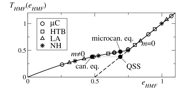
Figure 1: Caloric curve. The solid line is the Boltzmann-Gibbs equilibrium solution and the dashed line is the prolongation of the ordered phase to subcritical energies. Empty symbols are the average value of $e_{HMF}(t)$ at equilibrium. Full circles correspond to the QSS studied in the paper and to the subsequent microcanonical and canonical equilibrium obtained as $t\to\infty$.

2 Equilibrium simulations

The long-range interacting Hamiltonian considered in Refs. qss_literature,choi,hmf_can,hmf_qss is called Hamiltonian Mean Field (HMF) model and it can be thought as a set of $M$ globally coupled $XY$-spins with Hamiltonian

$$H_{HMF}=K_{HMF}+V_{HMF}=\sum_{i=1}^{M}\frac{l_{i}^{2}}{2}+\frac{1}{2M}\sum_{i,j=1}^{M}\left[1-\cos(\theta_{i}-\theta_{j})\right],$$ (1)

where $\theta_{i}\in[0,2\pi)$ are the spin angles assumed with unit momentum of inertia and $l_{i}\in\mathbb{R}$ their angular momenta (velocities). Its equilibrium statistical mechanics solution predicts an high-energy disordered phase separated from a low-energy ordered one by a second order transition occurring at the specific energy $e_{HMF}\equiv E_{HMF}/M=0.69$ (we use dimensionless units). The order parameter is the magnetization of the system $m_{HMF}\equiv|\sum_{i=1}^{M}(\cos\theta_{i},\sin\theta_{i})|/M$, and the presence of the kinetic term endows the spin system with a proper Hamiltonian dynamics in which one can define the temperature $T$ as twice the specific kinetic energy, $T_{HMF}\equiv 2K_{HMF}/M$. Notice the relation $e_{HMF}=(T_{HMF}+1-m_{HMF}^{2})/2$.

The Hamiltonian thermal bath (HTB) considered in Refs. hmf_can,hmf_qss is given by the full Hamiltonian system $H=H_{HMF}+H_{TB}+H_{I}$,

$$H_{TB} = \sum_{i=M+1}^{N}\frac{l_{i}^{2}}{2}+\sum_{i=M+1}^{N}\left[1-\cos(\theta_{i+1}-\theta_{i})\right],$$ (2)

$$H_{I} = \epsilon\sum_{i=1}^{M}\sum_{s=1}^{S}\left[1-\cos(\theta_{i}-\theta_{r_{s}(i)})\right],$$ (3)

where $H_{TB}$ and $H_{I}$ are respectively the Hamiltonian of the thermal bath and that of the interaction between HMF model and thermal bath ($N\gg M$). As the coupling constant $\epsilon$ vanishes, the $\mu$C dynamics of the HMF is recovered (see Ref. hmf_can for details).

A similar circumstance is valid for the LA thermostat where the equation of motion for the HMF model are

$$\ddot{\theta_{i}}=-\gamma\dot{\theta_{i}}-\sum_{j=1}^{M}\sin(\theta_{i}-\theta_{j})+\sqrt{2\gamma T}\;\xi_{i}(t),\quad i=1,2\ldots,M.$$ (4)

In Eq. (4) $\xi_{i}(t)$ is a Gaussian white noise characterized by a zero average $\langle\xi_{i}(t)\rangle=0$ and correlation $\langle\xi_{i}(t)\xi_{j}(t^{\prime})\rangle=\delta_{ij}\delta(t-t^{\prime})$. Indeed, in the limit $\gamma\to 0$, Eqs. (4) reduce to the $\mu$C Hamiltonian equations of the HMF model.

In Fig. 1 we present the results of the simulations in the different setups at equilibrium. These simulations are obtained by setting initial conditions close to equilibrium for the HMF model. Specifically, we used a Maxwellian distribution of velocities and an initial value of $m_{HMF}$ and of $T_{HMF}$ close to those of equilibrium for the given fixed energy ($\mu$C) or thermal bath temperature (HTB, NH and LA). After the relaxation to equilibrium, we verified that all the different dynamics give the same results for the values of the phase functions $e_{HMF}$, $T_{HMF}$ and $m_{HMF}$.

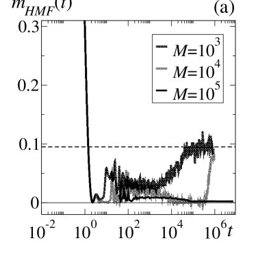
Figure 2: QSSs in $\mu$C simulations (a) and in HTB simulations with $\epsilon=0.01$ (b). Dashed lines are the equilibrium values for $m_{HMF}^{2}$. See Refs. 7,8 for further details.

3 Nonequilibrium simulations

The nonequilibrium analysis is performed by changing the initial conditions for the dynamical variables of the HMF model, while keeping all the other parameters unchanged with respect to the equilibrium results. Consistently with other studies reporting the existence of QSSs,[5] we have chosen at time $t=0$ a delta distribution for the angles [$p_{HMF}(\theta,0)=\delta(0)$ so that $m_{HMF}^{2}(0)=1$] and a uniform distribution for the velocities [$p_{HMF}(l,0)=1/2\bar{l},\;l\in[-\bar{l},\bar{l}]$, with $\bar{l}\simeq 2.03$]. In this way, the initial energy of the HMF model is set to the subcritical value $e_{HMF}(0)\simeq 0.69$.

The $\mu$C simulations reveal in this case the existence of a violent relaxation process[5] (for a time of order $1$) followed by a QSS which can be displayed e.g. by plotting the time dependence of $m_{HMF}^{2}$ (Fig. 2a). The QSS life-time diverges in the thermodynamic limit $M\to\infty$ and in this limit $m_{HMF}^{2}$ vanishes. The same kind of results are obtained using the HTB, although now the QSS life-time diminishes as $\epsilon$ increases (Fig. 2b). Notice that in the $\mu$C simulations the system relaxes to equilibrium at fixed energy, whereas in the HTB ones the relaxation is at fixed thermal bath temperature. This produces a consistent difference in the equilibrium values of $m_{HMF}^{2}$ (see also Fig. 1).

Unlike the results in the previous section, a NH integration scheme implemented with nonequilibrium initial conditions for the HMF model does not always guarantee the final convergence to equilibrium (Fig. 3). We found that only when $Q$ is larger then the value of the system size $M$ the convergence to equilibrium is realized. Still, the nonequilibrium dynamics is characterized by fluctuations of the phase functions which display no relation with the Hamiltonian simulations. Another drawback of the NH method is that if initially the HMF model has vanishing total momentum, this quantity remains zero during all the integrations steps.

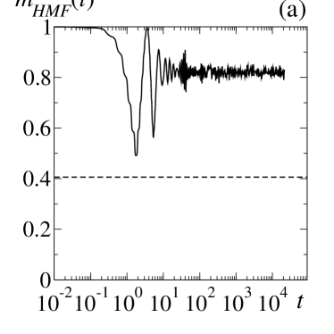
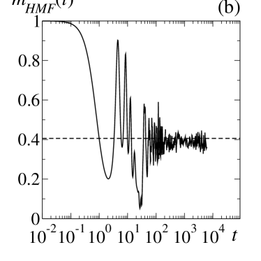
Figure 3: NH simulations with far-from-equilibrium initial conditions. (a) With $Q=1$ the magnetization does not converge to equilibrium. (b) With $Q=M=10^{3}$ the magnetization converges to equilibrium without displaying QSSs.

The analysis of the LA simulations reveals some interesting new results. In this case, as for the HTB, the convergence to equilibrium is observed for any value of $\gamma>0$ and the total momentum of the HMF model fluctuates during the simulation, as it is expected. Also, the violent relaxation process is coherently reproduced by the LA simulations and a QSS follows for which $m_{HMF}^{2}\to 0$ as $M$ grows. Nonetheless, the QSS life-time appears to be independent from the system size $M$ for any value of $\gamma>0$ (Fig. 4a). This life-time also shows an interesting dependence on $\gamma$. While the violent-relaxation time is of order $1$ independently on $\gamma$, the crossover time from the QSS to the equilibrium scales as $\gamma t$ (Fig. 4b). This scaling law implies an infinite life-time of the QSS in the $\mu$C limit $\gamma\to 0$, independently on $M$. Since such a result is in contrast with purely Hamiltonian $\mu$C simulations (Fig. 2a), it suggests the presence of a discontinuity in $\gamma=0$.

It is interesting to recall that a stability analysis of the Fokker-Planck equation derived from Eq. (4) shows that anomalous, non-Maxwellian, velocity probability density functions are (neutrally) stable only in the $\mu$C limit $\gamma=0$.[6] The somehow unexpected[6] presence of QSSs in LA simulations may be related to the fact that during the QSS the HMF model does not thermalize with the thermal bath (see Ref. hmf_qss,preparation for details).

In conclusion, by showing a specific example in which the NH and the LA thermostats simulations do not agree with the correspondent fully Hamiltonian ones, our findings constitute a general warning against the straightforward application of equilibrium-based algorithms for the description of the statistical nonequilibrium behavior.

Acknowledgments. FB acknowledges the organizers of the “International Conference on the Frontiers of Nonlinear and Complex Systems”, Hong Kong, May 2006, for generous support.

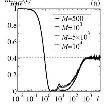
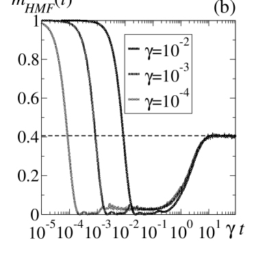
Figure 4: LA simulations with far-from-equilibrium initial conditions. (a) As $M$ increases, the QSS’s life-time remains constant. (b) The crossover time between QSS and equilibrium scales as $\gamma t$.

References

- [1] See, e.g., T. Dauxois, S. Ruffo, E. Arimondo, and M. Wilkens, Dynamics and Thermodynamics of Systems with Long Range Interactions, Lecture Notes in Physics Vol. 602 (Springer, New York, 2002).
- [2] See, e.g., R. Balescu, Statistical Dynamics (Imperial College Press, London, 1997).
- [3] See, e.g., M. Costeniuc, R. S. Ellis, H. Touchette, and B. Turkington, Phys. Rev. E 73, 026105 (2006) and references therein.
- [4] See, e.g., F. Borgonovi, G. L. Celardo, A. Musesti, R. Trasarti-Battistoni, and P. Vachal Phys. Rev. E 73, 026116 (2006) and references therein.
- [5] V. Latora, A. Rapisarda, and C. Tsallis Phys. Rev. E 64, 056134 (2001); A. Antoniazzi, D. Fanelli, J. Barré, P.H. Chavanis, T. Dauxois and S. Ruffo, Phys. Rev. E 75, 011112 (2007); Y.Y. Yamaguchi, J. Barré, F. Bouchet, T. Dauxois and S. Ruffo, Physica A 337, 36 (2004); F. Bouchet and T. Dauxois, Phys. Rev. E 72, 045103(R) (2005); P.H. Chavanis, Physica A 365, 102 (2006); T.M. Rocha Filho, A. Figueredo, and M.A. Amato, Phys. Rev. Lett. 95, 190601 (2005); See also, A. Pluchino and A. Rapisarda, Europhys. News 6, 202 (2005) and references therein;
- [6] M.Y. Choi and J. Choi, Phys. Rev. Lett. 91, 124101 (2003); J. Choi and M.Y. Choi, J. Phys. A 38, 5659 (2005); see also P.H. Chavanis, Physica A, 361, 55 (2006); Physica A, 361, 81 (2006).
- [7] F. Baldovin and E. Orlandini, Phys. Rev. Lett. 96, 240602 (2006).
- [8] F. Baldovin and E. Orlandini, Phys. Rev. Lett. 97, 100601 (2006).
- [9] D. Frenkel and B. Smit, Understanding Molecular Simulation (Academic Press, San Diego, 1996).
- [10] F. Baldovin and E. Orlandini, to be published.