Entropy of entanglement and correlations induced by a quench:
Dynamics of a quantum phase transition in the quantum Ising model

Abstract

Quantum Ising model in one dimension is an exactly solvable example of a quantum phase transition. We investigate its behavior during a quench caused by a gradual turning off of the transverse bias field. The system is then driven at a fixed rate characterized by the quench time $\tau_{Q}$ across the critical point from a paramagnetic to ferromagnetic phase. In agreement with Kibble-Zurek mechanism (which recognizes that evolution is approximately adiabatic far away, but becomes approximately impulse sufficiently near the critical point), quantum state of the system after the transition exhibits a characteristic correlation length $\hat{\xi}$ proportional to the square root of the quench time $\tau_{Q}$: $\hat{\xi}=\sqrt{\tau_{Q}}$. The inverse of this correlation length is known to determine average density of defects (e.g. kinks) after the transition. In this paper, we show that this same $\hat{\xi}$ controls the entropy of entanglement, e.g. entropy of a block of $L$ spins that are entangled with the rest of the system after the transition from the paramagnetic ground state induced by the quench. For large $L$, this entropy saturates at $\frac{1}{6}\log_{2}\hat{\xi}$, as might have been expected from the Kibble-Zurek mechanism. Close to the critical point, the entropy saturates when the block size $L\approx\hat{\xi}$, but – in the subsequent evolution in the ferromagnetic phase – a somewhat larger length scale $l=\sqrt{\tau_{Q}}\ln\tau_{Q}$ develops as a result of a dephasing process that can be regarded as a quantum analogue of phase ordering, and the entropy saturates when $L\approx l$. We also study the spin-spin correlation using both analytic methods and real time simulations with the Vidal algorithm. We find that at an instant when quench is crossing the critical point, ferromagnetic correlations decay exponentially with the dynamical correlation length $\hat{\xi}$, but (as for entropy of entanglement) in the following evolution length scale $l$ gradually develops. The correlation function becomes oscillatory at distances less than this scale. However, both the wavelength and the correlation length of these oscillations are still determined by $\hat{\xi}$. We also derive probability distribution for the number of kinks in a finite spin chain after the transition.

I Introduction

Phase transition is a fundamental change in the character of the state of a system when one of its parameters passes through the critical point. States on the opposite sides of the critical point are characterized by different types of ordering. In a second order phase transition, the fundamental change is continuous and the critical point is characterized by divergences in the coherence (or healing) length and in the relaxation time. This critical slowing down implies that no matter how slowly a system is driven through the transition its evolution cannot be adiabatic close to the critical point. If it were adiabatic, then the system would continuously evolve between the two types of ordering. However, in the wake of the necessarily non-adiabatic (and approximately impulse) evolution in the critical region, ordering of the state after the transition is not perfect: It is a mosaic of ordered domains whose finite size depends on the rate of the transition. This scenario was first described in the cosmological setting by Kibble K who appealed to relativistic casuality to set the size of the domains. The dynamical mechanism relevant for second order phase transitions was proposed by one of us Z . It is based on the universality of critical slowing down, and leads to prediction that the size of the ordered domains scales with the transition time $\tau_{Q}$ as $\tau_{Q}^{w}$, where $w$ is a combination of critical exponents. The Kibble-Zurek mechanism (KZM) for second order thermodynamic phase transitions was confirmed by numerical simulations of the time-dependent Ginzburg-Landau model KZnum and successfully tested by experiments in liquid crystals LC , superfluid helium 3 He3 , both high-$T_{c}$ highTc and low-$T_{c}$ lowTc superconductors and even in non-equilibrium systems ne . With the exception of superfluid ⁴He – where the early detection of copious defect formation He4a was subsequently attributed to vorticity inadvertently introduced by stirring He4b , and the situation remains unclear – experimental results are consistent with KZM, although more experimental work is clearly needed to allow for more stringent experimental tests of KZM.

The Kibble-Zurek mechanism is thus a universal theory of the dynamics of second order phase transitions whose applications range from the low temperature Bose-Einstein condensation (BEC) BEC to the ultra high temperature transitions in the grand unified theories of high energy physics. However, the zero temperature quantum limit remained unexplored until very recently, see Refs.3sites ; KZIsing ; Polkovnikov ; Dziarmaga2005 ; Levitov and an example of disordered system in Ref. random , and quantum phase transitions are in many respects qualitatively different from transitions at finite temperature. Most importantly time evolution is unitary, so there is no damping, and there are no thermal fluctuations that initiate symmetry breaking in KZM.

Quantum state of the many body system is indeed profoundly different from a classical state: Instead of a single broken symmetry configuration it may (and, generally, will) contain all of the possible configurations in a superposition. In addition to the ‘classical’ way of characterizing this state through the density of excitations (e.g. defects), one can wonder how entangled various parts of the system are with each other. Von Neumann entropy of a fragment due to its entanglement with the rest of the system is a convenient way to quantify this. It can be computed as a function of the size of the fragment. In equilibrium, and away from the critical point, this entropy of entanglement saturates at distances of the order of the coherence length $\xi$ of the system at values $\sim\ln\xi$ for one dimensional systems 18a . However, at the critical point (where equilibrium coherence length $\xi$ becomes infinite) entropy of entanglement diverges with the size of the fragment. In particular, in one dimensional systems, the critical entanglement entropy diverges logarithmically ($\sim\ln L$) with the length $L$ of the chain fragment 17a ; 17b ; 18a .

This equilibrium behavior suggests the question: What is the entanglement entropy left behind by an out-of-equilibrium phase transition? Such a transition will pass through the critical point (where entanglement entropy is logarithmically divergent) but this will happen at a finite rate set by the quench time $\tau_{Q}$. We show that the resulting entanglement entropy is of the order of $\sim\ln\hat{\xi}$, where $\hat{\xi}$ is the healing (coherence) length at the instant when critical slowing down forces the system to switch from the approximately adiabatic to approximately impulse (‘diabatic’) behavior. This suggests that the same process that determines the size of regions that “break symmetry in unison” (which sets the density of topological defects left by the transition) is also responsible for the resulting entanglement of formation left by the quench. This finding is consistent with recent results on quantum phase transitions induced by instantaneous quenches 18b ; 18c ; Instant which indicate that structures present in the initial pre-transition state determine the structures (and hence entanglement of formation) that arise after an instantaneous quench: Our results also suggest that – in accord with KZM – it is a good approximation to consider quench to be approximately adiabatic until the instant $\hat{t}\sim 1/\sqrt{\tau_{Q}}$ before the critical point is reached, and approximately impulse (e.g. nearly instantaneous) inside this time interval. This also confirms and extends results of the recent study of Cherng and Levitov Levitov who computed entropy density and correlations induced by quenches in one-dimensional chains, and concluded that their results support KZM.

While our results below are established for the one-dimensional quantum Ising model (which has the considerable advantage of being exactly solvable), we conjecture that similar behavior will be encountered in other quantum phase transitions, and that their non-equilibrium evolution can be anticipated using equilibrium critical exponents using KZM. This conjecture can be then tested in a variety of systems that undergo quantum phase transitions both in condensed matter and in atomic physics experiments.

According to Sachdev book , the understanding of quantum phase transitions is based on two prototypical models. One is the quantum rotor model and the other is the one-dimensional quantum Ising model. Of the two only the Ising model is exactly solvable. It is defined by the Hamiltonian

$$H~{}=~{}-\sum_{n=1}^{N}\left(g\sigma^{x}_{n}+\sigma^{z}_{n}\sigma^{z}_{n+1}\right)~{}.$$ (1)

with periodic boundary conditions

$$\vec{\sigma}_{N+1}~{}=~{}\vec{\sigma}_{1}~{}.$$ (2)

Quantum phase transition takes place at the critical value $g=1$ of an external magnetic field. When $g\gg 1$, the ground state is a paramagnet $|\rightarrow\rightarrow\rightarrow\dots\rightarrow\rangle$ with all spins polarized along the $x$-axis. On the other hand, when $g\ll 1$, then there are two degenerate ferromagnetic ground states with all spins pointing either up or down along the $z$-axis: $|\uparrow\uparrow\uparrow\dots\uparrow\rangle$ or $|\downarrow\downarrow\downarrow\dots\downarrow\rangle$. In an infinitesimally slow classical transition from paramagnet to ferromagnet, the system would choose one of the two ferromagnetic states. In the analogous quantum case, any superposition of these two states is also a ‘legal’ ground state providing it is consistent with other quantum numbers (e.g. parity) conserved by the transition from the initial paramagnetic state. However, when $N\to\infty$, then energy gap at $g=1$ tends to zero (quantum version of the critical slowing down) and it is impossible to pass the critical point at a finite speed without exciting the system. As a result, the system ends in a quantum superposition of states like

$$|\dots\uparrow\downarrow\downarrow\downarrow\downarrow\downarrow\uparrow\uparrow\uparrow\uparrow\uparrow\uparrow\uparrow\downarrow\downarrow\downarrow\downarrow\uparrow\uparrow\uparrow\uparrow\uparrow\uparrow\downarrow\dots\rangle$$ (3)

with finite domains of spins pointing up or down and separated by kinks where the polarization of spins changes its orientation. Average size of the domains or, equivalently, average density of kinks depends on a transition rate. When the transition is slow, then the domain size is large, but when it is very fast, then orientation of individual spins can become random, uncorrelated with their nearest neighbors. Transition time $\tau_{Q}$ can be unambiguously defined when we assume that close to the critical point at $g=1$ time-dependent field $g(t)$ driving the transition can be approximated by a linear quench

$$g(t<0)~{}=~{}-\frac{t}{\tau_{Q}}~{}.$$ (4)

with the adjustable quench time $\tau_{Q}$. Density of kinks after the linear quench was estimated in Ref. KZIsing showing that KZM can be also applied to quantum phase transitions. In this derivation, it is convenient to use instead of $g(t)$ a dimensionless parameter $\epsilon(t)=\frac{g-g_{c}}{g_{c}}=g-1$. As in classical transitions Z , one can assume the adiabatic-impulse approximation Bodzio ; Bodzio2 . The quench begins in the ground state at large initial $g$ and the initial part of the evolution is adiabatic: the state follows the instantaneous ground state of the system. The evolution becomes non-adiabatic close to the critical point when the energy gap $\simeq|\epsilon|$ becomes comparable to the instantaneous transition rate $|\dot{\epsilon}/\epsilon|$. This condition leads to an equation solved by $\hat{t}=\sqrt{\tau}_{Q}$ – the instant when the adiabatic to impulse transition occurs – which in turn yields $\hat{\epsilon}\simeq\tau_{Q}^{-1/2}$ and corresponds to the coherence length in the ground state Z ; KZIsing :

$$\hat{\xi}~{}=~{}\tau_{Q}^{1/2}~{}.$$ (5)

Assuming impulse approximation, the quantum state does not change during the following non-adiabatic stage of the evolution between $\hat{\epsilon}$ and $-\hat{\epsilon}$. Consequently, the quantum state at $-\hat{\epsilon}$ is expected to be approximately the ground state at $\hat{\epsilon}$ with the coherence length proportional to $\hat{\xi}$ and this is the initial state for the final adiabatic stage of the evolution after $\hat{\epsilon}$. This argument shows that when passing across the critical point, the state of the system gets imprinted with a finite KZ correlation length proportional to $\hat{\xi}$. In particular, this coherence length determines average density of kinks after the transition as

$$n~{}\simeq~{}\frac{1}{\tau_{Q}^{1/2}}~{}.$$ (6)

This is an order of magnitude estimate with an unknown ${\cal O}(1)$ prefactor. The estimate was verified by numerical simulations in Ref. KZIsing . Not much later the problem was solved exactly in Ref. Dziarmaga2005 , see also Ref. Levitov , with the exact solution confirming the KZM scaling in Eq. (6).

In the next section we review and expand the exact solution, and then use the expanded version to obtain a more complete set of results. In Subsection II.4, we derive Gaussian probability distribution for the number of kinks measured after a quench in a finite Ising spin chain. In Section III, we calculate entropy of entanglement of a block of $L$ spins after a dynamical transition and in Section IV we work out spin-spin correlation functions. We conclude in Section V.

II Exact solution

II.1 Energy spectrum

Here we assume that the number of spins $N$ is even for convenience. After the nonlocal Jordan-Wigner transformation JW ,

$$\sigma^{x}_{n}~{}=~{}1-2c^{\dagger}_{n}c_{n}~{},$$ (7)

$$\sigma^{z}_{n}~{}=~{}-\left(c_{n}+c_{n}^{\dagger}\right)\prod_{m<n}(1-2c^{\dagger}_{m}c_{m})~{},$$ (8)

introducing fermionic operators $c_{n}$ which satisfy anticommutation relations $\left\{c_{m},c_{n}^{\dagger}\right\}=\delta_{mn}$ and $\left\{c_{m},c_{n}\right\}=\left\{c_{m}^{\dagger},c_{n}^{\dagger}\right\}=0$ the Hamiltonian (1) becomes LSM

$$H~{}=~{}P^{+}~{}H^{+}~{}P^{+}~{}+~{}P^{-}~{}H^{-}~{}P^{-}~{}.$$ (9)

Above;

$$P^{\pm}=\frac{1}{2}\left[1\pm\prod_{n=1}^{N}\sigma^{x}_{n}\right]=\frac{1}{2}\left[1~{}\pm~{}\prod_{n=1}^{N}\left(1-2c_{n}^{\dagger}c_{n}\right)\right]$$ (10)

are projectors on the subspaces with even ($+$) and odd ($-$) numbers of $c$-quasiparticles and

$$H^{\pm}~{}=~{}\sum_{n=1}^{N}\left(gc_{n}^{\dagger}c_{n}-c_{n}^{\dagger}c_{n+1}-c_{n+1}c_{n}-\frac{g}{2}+{\rm h.c.}\right)~{}.$$ (11)

are the corresponding reduced Hamiltonians. The $c_{n}$’s in $H^{-}$ satisfy periodic boundary conditions $c_{N+1}=c_{1}$, but the $c_{n}$’s in $H^{+}$ must obey $c_{N+1}=-c_{1}$ – e.g, “antiperiodic” boundary conditions.

The parity of the number of $c$-quasiparticles is a good quantum number and the ground state has even parity for any non-zero value of $g$. Assuming that a quench begins in the ground state, we can confine to the subspace of even parity. $H^{+}$ is diagonalized by the Fourier transform followed by Bogoliubov transformation LSM . The Fourier transform consistent with the antiperiodic boundary condition $c_{N+1}=-c_{1}$ is

$$c_{n}~{}=~{}\frac{e^{-i\pi/4}}{\sqrt{N}}\sum_{k}c_{k}e^{ikn}~{},$$ (12)

where pseudomomenta $k$ take “half-integer” values:

$$k~{}=~{}\pm\frac{1}{2}\frac{2\pi}{N},\dots,\pm\frac{N-1}{2}\frac{2\pi}{N}~{}.$$ (13)

It transforms the Hamiltonian into

$$H^{+}~{} = \sum_{k}\left\{2[g-\cos(ka)]c_{k}^{\dagger}c_{k}+\right.$$ (14)

$$\left.\sin(ka)\left[c^{\dagger}_{k}c^{\dagger}_{-k}+c_{-k}c_{k}\right]-g\right\}~{}.$$

Diagonalization of $H^{+}$ is completed by the Bogoliubov transformation

$$c_{k}~{}=~{}u_{k}\gamma_{k}+v_{-k}^{*}\gamma^{\dagger}_{-k}~{},$$ (15)

provided that Bogoliubov modes $(u_{k},v_{k})$ are eigenstates of the stationary Bogoliubov-de Gennes equations

$$\epsilon~{}u_{k} = +2[g-\cos k]u_{k}+2\sin kv_{k}~{},$$

$$\epsilon~{}v_{k} = -2[g-\cos k]v_{k}+2\sin ku_{k}~{}.$$ (16)

There are two eigenstates for each $k$ with eigenenergies $\epsilon=\pm\epsilon_{k}$, where

$$\epsilon_{k}~{}=~{}2\sqrt{[g-\cos k]^{2}+\sin^{2}k}~{}.$$ (17)

The positive energy eigenstate

$$(u_{k},v_{k})\sim\left[(g-\cos k)+\sqrt{g^{2}-2g\cos k+1},\sin k\right]~{},$$ (18)

which has to be normalized so that $|u_{k}|^{2}+|v_{k}|^{2}=1$, defines the quasiparticle operator $\gamma_{k}~{}=~{}u_{k}^{*}c_{k}+v_{-k}c_{-k}^{\dagger}$, and the negative energy eigenstate $(u^{-}_{k},v^{-}_{k})=(-v_{k},u_{k})~{}$ defines $\gamma_{k}^{-}=(u_{k}^{-})^{*}c_{k}+v_{-k}^{-}c_{-k}^{\dagger}=-\gamma_{-k}^{\dagger}$. After the Bogoliubov transformation, the Hamiltonian $H^{+}=\frac{1}{2}\sum_{k}\epsilon_{k}\left(\gamma_{k}^{\dagger}\gamma_{k}-\gamma_{k}^{-\dagger}\gamma_{k}^{-}\right)$ is equivalent to

$$H^{+}~{}=~{}\sum_{k}\epsilon_{k}~{}\left(\gamma_{k}^{\dagger}\gamma_{k}-\frac{1}{2}\right)~{}.$$ (19)

This is a simple-looking sum of quasiparticles with half-integer pseudomomenta. However, thanks to the projection $P^{+}~{}H^{+}~{}P^{+}$ in Eq. (9) only states with even numbers of quasiparticles belong to the spectrum of $H$.

II.2 Linear quench

In the linear quench Eq. (4), the system is initially ($t\ll-\tau_{Q}$) in its ground state at large initial value of $g\gg 1$, but when $g$ is ramped down to zero, the system gets excited from its instantaneous ground state and, in general, its final state at $t=0$ has finite number of kinks. Comparing the Ising Hamiltonian Eq. (1) at $g=0$ with the Bogoliubov Hamiltonian (19) at $g=0$ we obtain a simple expression for the operator of the number of kinks

$${\cal N}~{}\equiv~{}\frac{1}{2}\sum_{n=1}^{N}\left(1-\sigma^{z}_{n}\sigma^{z}_{n+1}\right)~{}=~{}\sum_{k}\gamma_{k}^{\dagger}\gamma_{k}~{}.$$ (20)

The number of kinks is equal to the number of quasiparticles excited at $g=0$. The excitation probability

$$p_{k}~{}=~{}\langle\psi(0)|\gamma_{k}^{\dagger}\gamma_{k}|\psi(0)\rangle~{}$$ (21)

in the final state can be found with the time-dependent Bogoliubov method.

The initial ground state is Bogoliubov vacuum $|0\rangle$ annihilated by all quasiparticle operators $\gamma_{k}$ which are determined by the asymptotic form of the (positive energy) Bogoliubov modes $(u_{k},v_{k})\approx(1,0)$ in the regime of $g\gg 1$. When $g(t)$ is ramped down, the quantum state $|\psi(t)\rangle$ gets excited from the instantaneous ground state. The time-dependent Bogoliubov method makes an Ansatz that $|\psi(t)\rangle$ is a Bogoliubov vacuum annihilated by a set of quasiparticle annihilation operators $\tilde{\gamma}_{k}$ defined by a time-dependent Bogoliubov transformation

$$c_{k}~{}=~{}u_{k}(t)\tilde{\gamma}_{k}+v_{-k}^{*}(t)\tilde{\gamma}^{\dagger}_{-k}~{},$$ (22)

with the initial condition $[u_{k}(-\infty),v_{k}(-\infty)]=(1,0)$. In the Heisenberg picture, the Bogoliubov modes $[u_{k}(t),v_{k}(t)]$ must satisfy Heisenberg equation $i\hbar\frac{d}{dt}c_{k}~{}=~{}\left[c_{k},H^{+}\right]$ with the constraint that $\frac{d}{dt}\tilde{\gamma}_{k}=0$. The Heisenberg equation is equivalent to the dynamical version of the Bogoliubov-de Gennes equations (16):

$$i\hbar\frac{d}{dt}u_{k} = +2\left[g(t)-\cos k\right]u_{k}+2\sin k~{}v_{k}~{},$$

$$i\hbar\frac{d}{dt}v_{k} = -2\left[g(t)-\cos k\right]v_{k}+2\sin k~{}u_{k}~{}.$$ (23)

At any value of $g$, Eqs. (23) have two instantaneous eigenstates. Initially, the mode $[u_{k}(t),v_{k}(t)]$ is the positive energy eigenstate, but during the quench it gets “excited” to a combination of the positive and negative mode. At the end of the quench at $t=0$ when $g=0$ we have

$$\left[u_{k}(0),v_{k}(0)\right]=A_{k}\left(u_{k},v_{k}\right)+B_{k}\left(u_{k}^{-},v_{k}^{-}\right)$$ (24)

and consequently $\tilde{\gamma}_{k}=A_{k}\gamma_{k}-B_{k}\gamma_{k}^{\dagger}$. The final state which is, by construction, annihilated by both $\tilde{\gamma}_{k}$ and $\tilde{\gamma}_{-k}$ is

$$|\psi(0)\rangle=\prod_{k>0}\left(A_{k}+B_{k}\gamma^{\dagger}_{k}\gamma^{\dagger}_{-k}\right)|0\rangle~{}.$$ (25)

Pairs of quasiparticles with pseudomomenta $(k,-k)$ are excited with probability

$$p_{k}~{}=~{}|B_{k}|^{2}~{},$$ (26)

which can be found by mapping Eqs. (23) to the Landau-Zener (LZ) problem (similarity between KZM and LZ problem was first pointed out by Damski in Ref. Bodzio ).

The transformation

$$\tau~{}=~{}4\tau_{Q}\sin k\left(-\frac{t}{\tau_{Q}}+\cos k\right)$$ (27)

brings Eqs. (23) to the standard LZ form LZF

$$i\hbar\frac{d}{d\tau}u_{k} = -\frac{1}{2}(\tau\Delta_{k})u_{k}+\frac{1}{2}v_{k}~{},$$

$$i\hbar\frac{d}{d\tau}v_{k} = +\frac{1}{2}(\tau\Delta_{k})v_{k}+\frac{1}{2}u_{k}~{},$$ (28)

with $\Delta_{k}^{-1}=4\tau_{Q}\sin^{2}k$. Here the time $\tau$ runs from $-\infty$ to $\tau_{\rm final}=2\tau_{Q}\sin(2k)$ corresponding to $t=0$. Tunneling between the positive and negative energy eigenstates happens when $\tau\in(-\Delta_{k}^{-1},\Delta_{k}^{-1})$. $\tau_{\rm final}$ is well outside this interval, $\tau_{\rm final}\gg\Delta_{k}^{-1}$, for long wavelength modes with $|k|\ll\frac{\pi}{4}$. For these modes, time $\tau$ in Eqs. (28) can be extended to $+\infty$ making them fully equivalent to LZ equations LZF . This equivalence can be used to easily obtain several simple results Dziarmaga2005 described in the next subsection.

II.3 Simple results

In the limit of slow transitions we can assume that only long wavelength modes, which have small gaps at their anti-crossing points, can get excited. For these modes, we can use the LZ formula LZF for excitation probability:

$$p_{k}~{}\simeq~{}e^{-\frac{\pi}{2\Delta_{k}}}~{}\approx~{}e^{-2\pi\tau_{Q}k^{2}}~{}.$$ (29)

This approximation is self-consistent only when the width of the obtained Gaussian $(4\pi\tau_{Q})^{-1/2}$ is much less than $\frac{\pi}{4}$ or, equivalently, for slow enough quenches with $\tau_{Q}\gg 1$. With the LZ formula (29), we can calculate the number of kinks in Eq. (20) as

$${\cal N}~{}=~{}\sum_{k}~{}p_{k}~{}.$$ (30)

There are at least two interesting special cases:

• When $N\to\infty$ the sum in Eq. (30) can be replaced by an integral. The expectation value of density of kinks becomes

  $$n=\lim_{N\to\infty}\frac{\cal N}{N}=\frac{1}{2\pi}\int_{-\pi}^{\pi}dk~{}p_{k}=\frac{1}{2\pi}\frac{1}{\sqrt{2\tau_{Q}}}.$$ (31)

  The density scales like $\tau_{Q}^{-1/2}$ in agreement with KZM, see Eq. (6). Thus, slower quenches lead to fewer defects.

• Following Ref. KZIsing , we can ask what the fastest $\tau_{Q}$ is when no kinks get excited in a finite chain of size $N$. This critical $\tau_{Q}$ marks a crossover between adiabatic and non-adiabatic regimes. In other words, we can ask what is the probability for a finite chain is to stay in the ground state. As different pairs of quasiparticles $(k,-k)$ evolve independently, the probability to stay in the ground state is the product

  $${\cal P}_{\rm GS}~{}=~{}\prod_{k>0}\left(1-p_{k}\right)~{}.$$ (32)

  Well on the adiabatic side only the pair $\left(\frac{\pi}{N},-\frac{\pi}{N}\right)$ is likely to get excited and we can approximate

  $${\cal P}_{\rm GS}~{}\approx~{}1-p_{\frac{\pi}{N}}~{}\approx~{}1-\exp\left(-2\pi^{3}\frac{\tau_{Q}}{N^{2}}\right)~{}.$$ (33)

  A quench in a finite chain is adiabatic when

  $$\tau_{Q}~{}\gg~{}\frac{N^{2}}{2\pi^{3}}~{}.$$ (34)

  Reading this inequality from right to left, the size $N$ of a defect-free chain grows like $\tau_{Q}^{1/2}$. This is consistent with Eq. (6,31).

II.4 Probability distribution of the number of kinks

Equation (31) gives an average density of kinks measured after a quench to zero magnetic field $g=0$. In a finite chain, an average number of kinks is $\overline{\cal N}=Nn$, provided that the transition is non-adiabatic unlike in Eq. (34). The average $\overline{\cal N}$ is an expectation value of a probability distribution $P({\cal N})$ for the number of kinks ${\cal N}$ measured after a quench.

The number of kinks ${\cal N}$ is the number of quasiparticles excited by the end of the quench. As quasiparticles are excited in pairs with opposite quasimomenta $(k,-k)$, the number of kinks ${\cal N}$ must be even. A pair $(k,-k)$ is excited with the probability $p_{k}$ in Eq. (29). We can asign to each pair of quasiparticles a random variable $x_{k}$ which is $1$ when the pair is excited and $0$ otherwise: $x_{k}=1$ with probability $p_{k}$ and $x_{k}=0$ with probability $1-p_{k}$. We want a probability distribution for the sum ${\cal N}=\sum_{k>0}2x_{k}$. This is a sum of independent random variables of finite variance so for a large number of variables, the sum ${\cal N}$ becomes a Gaussian random variable with a mean $\overline{\cal N}=Nn$ and finite variance $\sim N$.

We have to be careful to specify when the number of random variables is large. Naively, on a $N$-site lattice, there are $N/2$ pairs of quasiparticles $(k,-k)$, or independent random variables $x_{k}$, and the number seems to be large when $N$ is large. On second thought, it is clear that variables with $p_{k}\approx 0$ or $p_{k}\approx 1$ cannot really count because they are hardly random at all. A look at the Gaussian $p_{k}$ in Eq. (29) shows that the range of $k>0$ where $0\ll p_{k}\ll 1$ has width $\simeq\frac{1}{\sqrt{\tau_{Q}}}$ which accommodates $\simeq\frac{N}{\sqrt{\tau_{Q}}}$ discrete values of pseudomomentum $k$. The relevant number of random variables is $\simeq\frac{N}{\sqrt{\tau_{Q}}}\simeq Nn=\overline{\cal N}$. It is large when the average number of kinks is large,

$$\overline{\cal N}~{}\gg~{}1~{}.$$ (35)

With this assumption $P(\cal N)$ is Gaussian.

Keeping this assumption in mind we can proceed as

$$P({\cal N}) = \sum_{x_{k}}~{}\delta_{{\cal N},\sum_{k>0}2x_{k}}$$ (37)

$$\prod_{k>0}\left[\delta_{0,x_{k}}(1-p_{k})+\delta_{1,x_{k}}p_{k}\right]~{}=$$

$$\frac{1}{2\pi}\int_{-\pi}^{\pi}dqe^{-iq{\cal N}}\prod_{k>0}\left[(1-p_{k})+p_{k}e^{2iq}\right]~{}\equiv$$

$$\frac{1}{2\pi}\int_{-\pi}^{\pi}dqe^{-iq{\cal N}}\tilde{P}(q)~{}.$$

It is convenient to evaluate first

$$\ln\tilde{P}(q) = \sum_{k>0}\ln\left[(1-p_{k})+p_{k}e^{2iq}\right]~{}\approx$$ (38)

$$\frac{N}{2\pi}\int_{0}^{\pi}dk~{}\ln\left[(1-p_{k})+p_{k}e^{2iq}\right]~{}.$$

Here we used $N\gg 1$, a necessary condition for our assumption that $\bar{\cal N}\gg 1$. After changing the integration variable to $u=\frac{k}{2\pi n}$, we can extend the integration over $u$ to infinity:

$$\ln\tilde{P}(q) = \overline{{\cal N}}\int_{0}^{\infty}du~{}\ln\left[(1-e^{-\pi u^{2}})+e^{-\pi u^{2}+2iq}\right]~{}\approx$$ (39)

$$\overline{{\cal N}}~{}\left(iq-\frac{\sqrt{2}-1}{\sqrt{2}}q^{2}\right)+{\cal O}(q^{3})~{}.$$

Here we used again $\overline{{\cal N}}=Nn$.

Finally, combination of Eqs. (39, 37) gives the expected Gaussian probability distribution

$$P\left({\cal N}\right) = \frac{1}{\sqrt{2\pi\sigma^{2}_{\cal N}}}\exp\left(-\frac{({\cal N}-\overline{\cal N})^{2}}{2\sigma^{2}_{\cal N}}\right)~{}.$$ (40)

with a variance

$$\sigma^{2}_{\cal N}~{}=~{}\left(2-\sqrt{2}\right)~{}\overline{\cal N}~{}.$$ (41)

In the course of our approximations, we have lost the constraint that ${\cal N}$ must be even, but this is not a big mistake when $\overline{{\cal N}}\gg 1$.

It is also interesting to study the opposite adiabatic regime when $Nn\ll 1$. When $\tau_{Q}$ is large we can approximate the product in Eq. (37) by a single factor with the lowest $k=\pi/N$,

$$P({\cal N}) \approx \sum_{s=0,1}\delta_{{\cal N},2s}~{}\left[\delta_{0,s}\left(1-p_{\pi/N}\right)+\delta_{1,s}p_{\pi/N}\right]~{}=$$ (42)

$$\delta_{{\cal N},0}~{}\left(1-p_{\pi/N}\right)~{}+~{}\delta_{{\cal N},2}~{}p_{\pi/N}~{}.$$

This is a good approximation when $\tau_{Q}~{}\gg~{}\frac{N^{2}}{2\pi^{3}}$ as in Eq. (34). In this adiabatic regime

$$\overline{\cal N}~{}=~{}2p_{\pi/N}~{}=~{}\exp\left(-2\pi^{3}\frac{\tau_{Q}}{N^{2}}\right)~{}.$$ (43)

The average number of kinks decays exponentially with $\tau_{Q}$ and the KZ power law scaling (31) does not extend to this adiabatic regime, as was already noted in Ref. KZIsing .

II.5 Exact solution and the two scales of length

So far we have avoided writing down solutions of the Landau-Zener equations (28) whose general form is, see e.g. Appendix B in Ref. Bodzio2 ,

$$v_{k}(\tau) = -\left[aD_{-s-1}(-iz)+bD_{-s-1}(iz)\right]~{},$$

$$u_{k}(\tau) = \left(-\Delta_{k}\tau+2i\frac{\partial}{\partial\tau}\right)v_{k}(\tau)~{},$$ (44)

with arbitrary complex parameters $a,b$. Here $D_{m}(x)$ is a Weber function, $s=\frac{1}{4i\Delta_{k}}$, and $z=\sqrt{\Delta_{k}}\tau e^{i\pi/4}$. The parameters $a,b$ are fixed by the initial conditions $u_{k}(-\infty)=1$ and $v_{k}(-\infty)=0$. Using the asymptotes of the Weber functions when $\tau\to-\infty$, we get $a=0$ and

$$|b|^{2}=\frac{e^{-\pi/8\Delta_{k}}}{4\Delta_{k}}~{}.$$ (45)

The solution of the linear quench problem is then

$$v_{k}(\tau) = -bD_{-s-1}(iz)~{},$$

$$u_{k}(\tau) = \left(-\Delta_{k}\tau+2i\frac{\partial}{\partial\tau}\right)v_{k}(\tau)~{},$$ (46)

At the end of the quench for $t=0$ and when $\tau=\tau_{k}=2\tau_{Q}\sin(2k)$, the argument of the Weber function $iz=\sqrt{\Delta_{k}}\tau e^{i\pi/4}=2\sqrt{\tau_{Q}}e^{i\pi/4}\cos(k){\rm sign}(k)$. In the limit of large $\tau_{Q}$ the modulus of this argument is large for most $k$, except the neighborhoods of $k=\pm\frac{\pi}{2}$, and we can again use the asymptotes of the Weber functions. After some work we get the products

$$|u_{k}|^{2} = \frac{1-\cos k}{2}+e^{-2\pi\tau_{Q}\sin^{2}k}~{},$$

$$|v_{k}|^{2} = 1-|u_{k}|^{2}~{},$$

$$u_{k}v_{k}^{*} = \frac{1}{2}\sin k+$$

$${\rm sign}(k)~{}e^{-\pi\tau_{Q}\sin^{2}k}\sqrt{1-e^{-\pi\tau_{Q}\sin^{2}k}}~{}e^{i\varphi_{k}}~{},$$

$$\varphi_{k} = \frac{\pi}{4}+\frac{\Delta_{k}\tau_{k}^{2}}{2}+\frac{\ln\Delta_{k}}{4\Delta_{k}}+\frac{\ln\tau_{k}}{2\Delta_{k}}-$$ (47)

$$\arg\left[\Gamma\left(1+\frac{i}{4\Delta_{k}}\right)\right]~{}.$$

Here $\Gamma(x)$ is the gamma function.

We expect that for large $\tau_{Q}$ only modes with small $|k|\ll\frac{\pi}{4}$ get excited. In this long wave length limit, the products can be further simplified to

$$|u_{k}|^{2} = \frac{1-\cos k}{2}+e^{-2\pi\tau_{Q}k^{2}}~{},$$

$$|v_{k}|^{2} = 1-|u_{k}|^{2}~{},$$

$$u_{k}v_{k}^{*} = \frac{1}{2}\sin k+{\rm sign}(k)~{}e^{-\pi\tau_{Q}k^{2}}\sqrt{1-e^{-\pi\tau_{Q}k^{2}}}~{}e^{i\varphi_{k}}~{},$$

$$\varphi_{k} = \frac{\pi}{4}+2\tau_{Q}-(2-\ln 4)\tau_{Q}k^{2}+$$ (48)

$$k^{2}\tau_{Q}\ln\tau_{Q}-\arg\left[\Gamma\left(1+i\tau_{Q}k^{2}\right)\right]~{}.$$

These products depend on $k$ and $\tau_{Q}$ through two combinations: $\tau_{Q}k^{2}$, which implies the usual KZM coherence length $\hat{\xi}=\sqrt{\tau_{Q}}$, and $k^{2}\tau_{Q}\ln\tau_{Q}$ which implies a second length scale $\sqrt{\tau_{Q}\ln\tau_{Q}}$. The final quantum state at $g=0$ cannot be characterized by a single scale of length. Physically, this appears to reflect a combination of two processes: KZM that sets up initial post-transition state of the system, and the subsequent evolution that can be regarded as quantum phase ordering.

III Entropy of a block of spins

Von Neumann entropy of a block of $L$ spins due to its entanglement with the rest of the system;

$$S(L)~{}=~{}-~{}{\rm Tr}~{}\rho_{L}~{}\log_{2}\rho_{L}~{},$$ (49)

is a convenient measure of entanglement. Above $\rho_{L}$ is reduced density matrix of the subsystem of $L$ spins. In recent years this entropy was studied extensively in ground states of quantum critical systems 17b ; 17c ; 17d ; 17e ; 18a ; 18b ; 18c ; JStatPhys . At a quantum critical point, the entropy diverges like $\log L$ for large $L$ with a prefactor determined by the central charge of the relevant conformal field theory 17a ; 17b ; 18a . In particular, in the quantum Ising model at the critical $g=1$

$$S^{\rm GS}(L)~{}\simeq~{}\frac{1}{6}\log_{2}L~{}$$ (50)

for large $L$. Slightly away from the critical point, the entropy saturates at a finite asymptotic value 18a

$$S_{\infty}^{\rm GS}~{}\simeq~{}\frac{1}{6}\log_{2}\xi$$ (51)

when the block size $L$ exceeds the finite correlation length $\xi$ in the ground state of the system.

III.1 Entropy after dynamical transition

In a dynamical quantum phase transition the quantum state of the system developes a finite correlation length $\hat{\xi}\simeq\sqrt{\tau_{Q}}$. If this dynamical correlation length were the only relevant scale of length, then one could expect entropy of entanglement after a dynamical transition given by Eq. (51) with $\xi$ simply replaced by $\hat{\xi}$. However, as we saw in Eq. (48), there are two scales of length, and – strictly speaking – there is no reason to expect that either of them alone is relevant in general. This is why we shall not rely on scaling arguments alone and will go on to calculate the entropy of entanglement “from scratch”.

We proceed in a similar way as in Ref. 17b ; 17c ; 17e ; 18b ; JStatPhys and define a correlator matrix for the block of $L$ spins

$$\Pi~{}=~{}\left(\begin{array}[]{ccc}\alpha&,&\beta^{\dagger}\\ \beta&,&1-\alpha\end{array}\right)~{},$$ (52)

where $\alpha$ and $\beta$ are $L\times L$ matrices of quadratic correlators

$$\alpha_{m,n} \equiv \langle c_{m}c_{n}^{\dagger}\rangle=$$ (53)

$$\frac{1}{2\pi}\int_{-\pi}^{\pi}dk~{}|u_{k}|^{2}~{}e^{ik(m-n)}~{}\stackrel{{\scriptstyle\tau_{Q}\gg 1}}{{\approx}}$$

$$\frac{1}{2}\delta_{0,|m-n|}-\frac{1}{4}\delta_{1,|m-n|}+\frac{e^{-\frac{(m-n)^{2}}{8\pi~{}\hat{\xi}^{2}}}}{2\sqrt{2}\pi~{}\hat{\xi}}~{}.$$

and

$$\beta_{m,n}~{}\equiv~{}\langle c_{m}c_{n}\rangle=$$

$$\frac{1}{2\pi i}\int_{-\pi}^{\pi}dk~{}u_{k}v_{k}^{*}~{}e^{ik(m-n)}~{}=$$

$$\frac{1}{\pi}\int_{0}^{\pi}dk~{}u_{k}v_{k}^{*}~{}\sin k(m-n)~{}\stackrel{{\scriptstyle\ln\tau_{Q}\gg 1}}{{\approx}}$$ (54)

$${\rm sign}(m-n)~{}\times$$

$$\left[\frac{1}{4}\delta_{1,|m-n|}-\frac{e^{i\left(2\tau_{Q}-\frac{|m-n|^{2}}{4~{}\hat{\xi}l}\right)}}{2\sqrt{\pi~{}\hat{\xi}~{}l}}e^{-\frac{\pi|m-n|^{2}}{4~{}l^{2}}}\sqrt{1-e^{-\frac{\pi|m-n|^{2}}{4~{}l^{2}}}}\right]$$

Here $\hat{\xi}=\sqrt{\tau_{Q}}$ is the KZM dynamical correlation length and

$$l~{}\equiv~{}\sqrt{\tau_{Q}}\ln\tau_{Q}~{}.$$ (55)

We note that $\alpha$ and $\beta$ are Toeplitz matrices with constant diagonals. The expectation values $\langle\dots\rangle$ are taken in the dynamical Bogoliubov vacuum state. As this state is Gaussian, all higher order correlators can be expressed by the matrices $\alpha$ and $\beta$ - they provide complete characterization of the quantum state after the dynamical transition. The matrices depend on both scales $\hat{\xi}$ and $l$ and both scales are necessary to characterize the Gaussian state.

As observed in Ref. 17b ; 17c ; 17e ; 18b ; JStatPhys , the entropy can be conveniently calculated as

$$S(L,\tau_{Q})~{}=~{}-~{}{\rm Tr}~{}\rho~{}\log_{2}\rho~{}=~{}-~{}{\rm Tr}~{}\Pi~{}\log_{2}\Pi~{}.$$ (56)

In this calculation we use Eq. (47) and Eqs. (53, 54) but without their large $\tau_{Q}$ approximations. The calculation involves a numerical evaluation of the integrals in Eqs. (53,54) and numerical diagonalization of the matrix $\Pi$. Results are shown in Panel A of Fig.1. The entropy grows with the block size $L$ and saturates at a finite value $S_{\infty}(\tau_{Q})$ for large enough $L$. In Panel B, we fit the asymptotic entropy with the linear function $S_{\infty}(\tau_{Q})=A+B\ln\tau_{Q}$. The simple replacement of $\xi$ by $\hat{\xi}=\sqrt{\tau_{Q}}$ in Eq. (51) suggests the asymptotic value

$$S_{\infty}(\tau_{Q})~{}\simeq~{}\frac{1}{6}\log_{2}\hat{\xi}~{}\simeq~{}\frac{\ln 2}{12}~{}\ln\tau_{Q}~{}=~{}0.120~{}\ln\tau_{Q}~{}.$$ (57)

Our best fit gives $B=0.128\pm 0.004$ and $A=1.80\pm 0.05$. The best $B$ is in reasonably good agreement with the expected value of $0.120$.

In Panels C and D of the same figure, we rescale values of entropy $S(L,\tau_{Q})$ by its asymptotic value $S_{\infty}(\tau_{Q})\approx A+B\ln\tau_{Q}$. After this transformation we can better focus on how the entropy depends on the block size $L$. A simple hypothesis would be that entropy depends on $\hat{\xi}$ and saturates when $L>\hat{\xi}$. To check if this is true, in Panel C we also rescale the block size $L$ by $\hat{\xi}=\sqrt{\tau_{Q}}$ and find that while this rescaling brings plots close to overlap, they do not overlap as well as one might have hoped. By contrast, as shown in Panel D, rescaling of the block size $L$ by $l=\sqrt{\tau_{Q}}\ln\tau_{Q}$ makes the multiple plots overlap quite well indeed. In conclusion, our results support the statement that the entropy saturates at

$$S_{\infty}(\tau_{Q})~{}\simeq~{}\frac{1}{6}~{}\log_{2}\sqrt{\tau_{Q}}~{}$$ (58)

when

$$L~{}\gg~{}\sqrt{\tau_{Q}}\ln\tau_{Q}~{}$$ (59)

i.e. the entropy of a large block of spins is determined by Kibble-Zurek dynamical correlation length $\hat{\xi}=\sqrt{\tau_{Q}}$, but the entropy saturates when the block size is greater than the second scale $l=\sqrt{\tau_{Q}}\ln\tau_{Q}$.

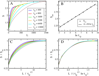
Figure 1: Panel A shows entropy of a block of $L$ spins after the dynamical phase transition as a function of the block size $L$. The multiple plots correspond to different values of the quench time $\tau_{Q}$. For all $\tau_{Q}$, the entropy grows with the block size $L$ and saturates at a finite value $S_{\infty}(\tau_{Q})$ for large enough $L$. In Panel B, we fit this asymptotic value of entropy with the function $S_{\infty}(\tau_{Q})=A+B\ln\tau_{Q}$. The best fit has $B=0.128\pm 0.004$ and $A=1.80\pm 0.05$. This $B$ is in reasonably good agreement with the expected value of $B=\frac{\ln 2}{12}=0.120$. In Panels C and D, we rescale values of entropy $S(L,\tau_{Q})$ by the best fit to its asymptotic value $S_{\infty}(\tau_{Q})=A+B\ln\tau_{Q}$. With this rescaling we can focus on how the entropy depends on the block size $L$. In Panel C, we also rescale the block size by $\hat{\xi}=\sqrt{\tau_{Q}}$ and find that the rescaled plots do not overlap exactly. However, as shown in Panel D, rescaling the block size $L$ by the second scale $l=\sqrt{\tau_{Q}}\ln\tau_{Q}$ makes the six plots overlap quite well.

We believe that the KZ correlation length $\hat{\xi}$ is determined when the system is crossing the critical point while the second longer scale builds up after the system gets excited from its adiabatic ground state near the critical value of a magnetic field. At the origin of the second scale is the non-trivial dispersion relation of excited quasiparticles. The $k$-dependent $\epsilon_{k}$ in Eq. (17) leads to a gradual evolution of matrix elements of the correlator $\Pi$ which are given by integrals over $k$ in Eqs. (53,54). To support this scenario we calculated the entropy of entanglement at the moment when the system is crossing the critical point at $g=1$. The results collected in Figure 2 are consistent with our expectation that near the critical point, when the scale $l$ set up by quantum phase ordering only begins to build up, $\hat{\xi}$ is still the only relevant scale of length.

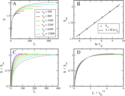
Figure 2: Panel A shows entropy of a block of $L$ spins during the dynamical phase transition at the critical point $g=1$ as a function of the block size $L$. The multiple plots correspond to different values of the quench time $\tau_{Q}$. For all the quench times, the entropy grows with the block size $L$ and saturates at a finite value $S_{\infty}(\tau_{Q})$ for large enough $L$. In Panel B we fit this asymptotic value of entropy with the function $S_{\infty}(\tau_{Q})=A+B\ln\tau_{Q}$. The best fit has $B=0.126\pm 0.005$ and $A=0.80\pm 0.03$. This $B$ is in reasonably good agreement with the expected value of $B=\frac{\ln 2}{12}=0.120$. In Panels C and D, we rescale the entropy $S(L,\tau_{Q})$ by the best fit to its asymptotic value $S_{\infty}(\tau_{Q})\approx A+B\ln\tau_{Q}$. With this rescaling we can focus on how the entropy depends on the block size $L$. In Panel D, rescaling the block size $L$ by $\hat{\xi}=\sqrt{\tau_{Q}}$ makes the six plots overlap quite well.

III.2 Impurity of the state after transition

We were not able to do a fully analytic calculation of entropy. This is why it may be worthwhile to calculate analytically another more easily tractable entanglement-related quantity. For example, the “impurity” of the correlator matrix $\Pi$

$$I(\Pi)~{}=~{}{\rm Tr}~{}\Pi~{}(1-\Pi)$$ (60)

is zero only when the $L$ spins are in a pure state i.e. when all eigenvalues of $\Pi$ are either $0$ or $1$. It is maximal when all the eigenvalues are $\frac{1}{2}$, or when the state is most entangled. Thanks to its simple quadratic form, it can be calculated relatively easily.

Simple calculation using the block structure of $\Pi$ in Eq. (52) and the Toeplitz property of the block matrices $\alpha$ and $\beta$ leads to

$$I\left(L\right)~{}=~{}2\left(L\alpha_{0}-\sum_{j=1-L}^{j=L-1}(L-|j|)(\alpha_{j}^{2}+|\beta_{j}|^{2})\right),$$ (61)

where $\alpha_{j}=\alpha_{j,0}$ and $\beta_{j}=\beta_{j,0}$. $\alpha_{j}$ and $\beta_{j}$ can be expressed by the inverse Fourier transforms in Eqs. (53,54). Using normalization $|u_{k}|^{2}+|v_{k}|^{2}=1$ and completeness of the Fourier basis we notice that

$$\alpha_{0} = \frac{1}{2\pi}\int_{-\pi}^{\pi}dk~{}|u_{k}|^{2}=$$

$$\frac{1}{2\pi}\int_{-\pi}^{\pi}dk~{}(|u_{k}|^{4}+|u_{k}v_{k}^{*}|^{2})=$$

$$\sum_{j=-\infty}^{j=\infty}(|\beta_{j}|^{2}+|\alpha_{j}|^{2}).$$

This leads to

$$I\left(L\right)=4L\sum_{j=L}^{\infty}(|\beta_{j}|^{2}+|\alpha_{j}|^{2})+4\sum_{j=1}^{L-1}j(|\beta_{j}|^{2}+|\alpha_{j}|^{2}).$$ (63)

Since we assume that $\tau_{Q}\gg 1$, we can approximate these sums with integrals. Further calculation gives:

$$I\left(L\right) = \frac{1}{2}+\frac{1}{\pi}\left(1-e^{-\frac{(L-1)^{2}}{4\pi\tau_{Q}}}\right)+$$

$$\frac{\ln(\tau_{Q})}{2\pi^{2}}\left(1-e^{-\frac{\pi(L-1)^{2}}{2\tau_{Q}(\ln\tau_{Q})^{2}}}\right)^{2}-\frac{1}{\pi\sqrt{2\tau_{Q}}}+$$

$$\frac{L}{2\pi\sqrt{\tau_{Q}}}\left[\mathrm{Erfc}\left(\frac{L}{\sqrt{4\pi\tau_{Q}}}\right)+\right.$$

$$\left.\sqrt{2}\mathrm{\mathrm{Erfc}}\left(\frac{L\sqrt{\pi}}{\sqrt{2\tau_{Q}}\ln\tau_{Q}}\right)-\mathrm{Erfc}\left(\frac{L\sqrt{\pi}}{\sqrt{\tau_{Q}}\ln\tau_{Q}}\right)\right].$$

Here $\mathrm{Erfc}(x)$ is the complementary error function defined as:

$$\mathrm{Erfc}(x)=\frac{2}{\sqrt{\pi}}\int_{x}^{\infty}e^{-t^{2}}dt.$$ (65)

This impurity saturates at $I_{\infty}\simeq\ln\tau_{Q}$ when the block size $L\gg l$, or in short

$$I_{\infty}~{}\approx~{}\frac{\ln\tau_{Q}}{2\pi^{2}}~{}.$$ (66)

The impurity saturates at the second scale $l=\sqrt{\tau_{Q}}\ln\tau_{Q}$ in consistency with our results for the entropy.

It is interesting to compare the dynamical impurity (66) with the impurity in the ground state of the system. Simple calculation gives the asymptote of impurity in the ground state at the critical point

$$I^{\rm GS}(L)~{}=~{}\frac{\ln L}{\pi^{2}}~{}.$$ (67)

when $\ln L\gg 1$. Near the critical point, the asymptote is valid for the block size $L$ much less than the correlation function $L\ll\xi$ and at larger $L$ the impurity saturates at

$$I^{\rm GS}_{\infty}~{}\simeq~{}\frac{\ln\xi}{\pi^{2}}~{}.$$ (68)

Simple replacement of $\xi$ in this equation by the dynamical KZ correlation length $\hat{\xi}=\sqrt{\tau_{Q}}$ gives the asymptotic value of the dynamical impurity in Eq. (66). Again, this “replacement rule” is the same as for the entropy.

IV Correlation functions

Correlation functions are of fundamental interest in phase transitions because they provide direct manifestation of their universal properties and are in general easily accesible experimentally. In this Section we present our results for spin-spin correlation functions during a dynamical quantum phase transition.

To begin with, we observe that for symmetry reasons the magnetization $\langle\sigma^{z}\rangle=0$, but the transverse magnetization

$$\langle\sigma^{x}_{n}\rangle~{}=~{}\langle 1-2c^{\dagger}_{n}c_{n}\rangle~{}=~{}2\alpha_{0}-1~{}\approx~{}\frac{1}{2\pi\sqrt{2\tau_{Q}}}~{},$$ (69)

which is valid when $\tau_{Q}\gg 1$. This is what remains of the initial magnetization $\langle\sigma^{x}_{n}\rangle=1$ in the initial ground state at $g\to\infty$. As expected, when the linear quench is slow, then the final magnetization decays towards $\langle\sigma^{x}_{n}\rangle=0$ characteristic of the ground state at the final $g=0$.

Final transverse spin-spin correlation function at $g=0$ is

$$C^{xx}_{R} \equiv \langle\sigma^{x}_{n}\sigma^{x}_{n+R}\rangle-\langle\sigma^{x}_{n}\rangle\langle\sigma^{x}_{n+R}\rangle~{}=~{}$$ (71)

$$4\left(|\beta_{R}|^{2}-|\alpha_{R}|^{2}\right)~{}\approx$$

$$\frac{e^{-\frac{\pi R^{2}}{2~{}l^{2}}}\left(1-e^{-\frac{\pi R^{2}}{4~{}l^{2}}}\right)}{\pi~{}\hat{\xi}~{}l}-\frac{e^{-\frac{R^{2}}{\pi~{}\hat{\xi}^{2}}}}{2\pi^{2}~{}\hat{\xi}^{2}}~{},$$

when $R>1$ and $\ln\tau_{Q}\gg 1$. This correlation function depends on both $\hat{\xi}$ and $l$. Long range correlations

$$C^{xx}_{R}~{}\sim~{}e^{-\frac{\pi R^{2}}{2~{}l^{2}}}$$ (72)

decay in a Gaussian way on the scale $l$.

IV.1 Ferromagnetic correlations at $g=0$

In contrast, the ferromagnetic spin-spin correlation function

$$C^{zz}_{R}~{}=~{}\langle\sigma^{z}_{n}\sigma^{z}_{n+R}\rangle~{}-~{}\langle\sigma^{z}_{n}\rangle\langle\sigma^{z}_{n+R}\rangle~{}=~{}\langle\sigma^{z}_{n}\sigma^{z}_{n+R}\rangle$$ (73)

cannot be evaluated so easily. As is well known, in the ground state, $C^{zz}_{R}$ can be written as a determinant of an $R\times R$ Toeplitz matrix whose asymptote for large $R$ can be obtained with the Szego limit theorem Schogo . Unfortunately, in time-dependent problems the correlation function is not a determinant in general. However, below we avoid this problem in an interesting range of parameters.

Using the Jordan-Wigner transformation, $C^{zz}_{R}$ can be expressed as

$$C^{zz}_{R}~{}=~{}\langle b_{0}a_{1}b_{1}a_{2}\ldots b_{R-1}a_{R}\rangle~{}.$$ (74)

Here $a_{n}$ and $b_{n}$ are Majorana fermions defined as $a_{n}=(c_{n}^{\dagger}+c_{n})$ and $b_{n}=c_{n}^{\dagger}-c_{n}$. Using (53) and (54) we get:

$$\langle a_{m}b_{n}\rangle = 2\alpha_{n-m}+2\Re\beta_{n-m}-\delta_{m,n}$$

$$\langle b_{m}a_{n}\rangle = \delta_{m,n}-2\alpha_{n-m}+2\Re\beta_{n-m}$$ (75)

$$\langle a_{m}a_{n}\rangle = \delta_{m,n}+2\imath\Im\beta_{m-n}$$

$$\langle b_{m}b_{n}\rangle = \delta_{m,n}+2\imath\Im\beta_{m-n}$$

The average in Eq. (74) is a determinant of a matrix when $\langle a_{m}a_{n}\rangle=0$ and $\langle b_{m}b_{n}\rangle=0$ for $m\neq n$, or equivalently when $\Im\beta_{m-n}=0$ for $m\neq n$. Inspection of the last line in Eq. (54) shows that $\Im\beta_{m-n}\approx 0$ when $|m-n|\ll l$. Consequently, when the correlation distance $R\ll l$ we can neglect all $\Im\beta_{m-n}$ assuming that $\langle a_{m}a_{n}\rangle=0$ and $\langle b_{m}b_{n}\rangle=0$ for $m\neq n$. In this regime, the correlation function is a determinant of the Toeplitz matrix

$$\left[\langle b_{m}a_{n+1}\rangle\right]_{m,n=1,\ldots,R}~{}.$$ (76)

Asymptotic behavior of this Toeplitz determinant can be obtained using standard methods Schogo with the result that

$$C^{zz}_{R}~{}\sim~{}\exp\left(-0.174~{}\frac{R}{\hat{\xi}}\right)~{}\cos\left(\sqrt{\frac{\log 2}{2\pi}}~{}\frac{R}{\hat{\xi}}-\varphi\right)$$ (77)

when $1\ll R\ll l$.

In this way we find that the final ferromagnetic correlation function at $g=0$ exhibits decaying oscillatory behavior on length scales much less than the phase - ordered scale $l$, but both the wavelength of these oscillations and their exponentially decaying envelope are determined by $\hat{\xi}$. As discussed in a similar situation by Cherng and Levitov Levitov , this oscillatory behavior means that consecutive kinks are approximately anticorrelated – they keep more or less the same distance $\simeq\hat{\xi}$ from each other forming something similar to a …-kink-antikink-kink-antikink-… lattice with a lattice constant $\simeq\hat{\xi}$. However, fluctuations in the length of bonds in this lattice are comparable to the average distance itself giving the exponential decay of the correlator $C^{zz}_{R}$ on the same scale of $\simeq\hat{\xi}$.

We do not know the tail of the ferromagnetic correlation function when $L\gg l$ because our approximations necessary to derive Eq. (77) do not work in this regime, but we can estimate that this tail is not negligible. Indeed, when $R=l$, then the envelope in Eq. (77) is

$$\exp\left(-0.174~{}\frac{l}{\hat{\xi}}\right)~{}=~{}e^{-0.174\ln\tau_{Q}}~{}=~{}\tau_{Q}^{-0.174}~{}.$$ (78)

Due to the smallness of the exponent $0.174$ the tail is negligible only for extremely large $\tau_{Q}$.

IV.2 Correlations at the critical point

In order to fill in the gaps in our analytic knowledge of the correlation functions, we attempted to make numerical simulations of the dynamical transition. As we wanted to get information on spin-spin correlation functions it proved convenient to work directly with spin degrees of freedom rather than with the Jordan-Wigner fermions. We used the translationally invariant version of the real time Vidal algorithm Vidal . This algorithm, which is an elegant version of the density matrix renormalization group DMRG , is an efficient way to simulate time evolution of an infinite translationally invariant spin chain. This ambitious task is made efficient by a clever truncation of Schmidt decomposition between any two halves of the infinite spin chain. Our calculations of the entropy of entanglement demonstrate that for a finite transition rate, the entropy saturates at a finite value beyond certain block size $L$. This saturation suggests that in our case the truncation of the Schmidt decomposition will make sense and, in principle, dynamical phase transitions across quantum critical points can be efficiently simulated with the Vidal algorithm.

In our simulations, we started the linear quench from the ground state at $g=10$ which was prepared with the imaginary time version of the algorithm. The simulations were run for a range of $\tau_{Q}$ such that the initial part of the evolution close to $g=10$ was well in the adiabatic regime. We checked our results for convergence with respect to the truncation of the Schmidt decomposition (we used $\chi$ up to $\chi=40$) and time step $dt$. We used fourth order Trotter decomposition. Wherever it was possible, we compared our numerical results with analytical results which could be obtained for transversal magnetization, transversal spin-spin correlations, and ferromagnetic nearest-neighbor correlations. We also controlled if our truncation of the Schmidt decomposition is sufficient to preserve the norm of the state evolved in real time. As illustrated in panel A of Figure 3, our simulations were stable enough to cross the critical point and enter the ferromagnetic phase, but once in the ferromagnetic phase, the algorithm was breaking down. This is why we trust our numerical results at $g=1$, but have no reliable results below $g=1$. We can verify KZM at the critical point, but we cannot reliably follow the phase ordering in the ferromagnetic phase.

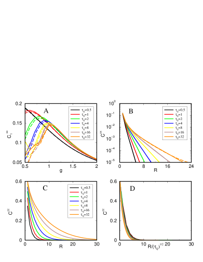
Figure 3: Panel A shows the dynamical transverse correlation $C^{xx}_{1}$ as a function of magnetic field $g$ in the linear quench. For each $\tau_{Q}$, we show both numerical (dashed) and analytical (solid) result. The plots overlap near the critical point at $g=1$ but diverge in the ferromagnetic phase when $g<1$ indicating a breakdown of our numerical simulations in this regime. Panel B shows analytic and numerical results for the dynamical transverse correlation function at the moment when the quench crosses the critical point at $g=1$. The transverse correlators overlap well confirming that our numerical simulations are still accurate at the critical point. Finally, in panel C, we show the dynamical ferromagnetic correlation function $C^{zz}_{R}$ at $g=1$ and in panel D, we show the same correlation function after rescaling $R/\sqrt{\tau_{Q}}$. The rescaled plots overlap quite well supporting the idea that near the critical point the KZ correlation length $\hat{\xi}=\sqrt{\tau_{Q}}$ is the only relevant scale of length.

In panel B of Figure 3, we plot the transverse spin-spin correlation $C^{xx}_{R}$ at $g=1$ for several values of $\tau_{Q}$. For each $\tau_{Q}$, we plot both numerical correlator and its analytic counterpart from Eq. (71) and they seem to approximately coincide. Equation (71) can be also used to obtain analytically, but with some numerical integration, the exponential tail of the transverse correlator when $\tau_{Q}\gg 1$:

$$C^{xx}_{R} \approx \frac{0.44}{\tau_{Q}}~{}\exp\left(-2.03\frac{R}{\hat{\xi}}\right)$$ (79)

accurate when $R\gg\hat{\xi}$. This tail decays on the KZ correlation length $\hat{\xi}$ which proves to be the relevant scale of length.

Encouraged by the agreement in transverse correlations in panel C we show the ferromagnetic spin-spin correlation functions at $g=1$ for the same values of $\tau_{Q}$. They are roughly exponential and their correlation length seems to be set by $\hat{\xi}=\sqrt{\tau_{Q}}$. To verify this scaling hypothesis we show in panel D the same plots as in panel C but with $R$ rescaled as $R/\hat{\xi}$. We find the rescaled plots to overlap reasonably well confirming the expected $\sqrt{\tau_{Q}}$ scaling. The overlap is not perfect, but the scaling is expected when $\tau_{Q}\gg 1$ which is not quite satisfied by the $\tau_{Q}$ available from our numerical simulations.

V Conclusion

Putting our analytical results and numerical evidence together, we are led to conclude that, in a quantum phase transition, the system initially follows adiabatically its instantaneous ground state. This adiabatic behavior becomes impossible sufficiently near the critical point: When crossing the critical regime the system gets excited in a manner consistent with KZM, and imprinted with the characteristic KZ dynamical correlation length $\hat{\xi}=\sqrt{\tau_{Q}}$. We find evidence for this correlation length both in correlation functions and in the entropy of entanglement - they are all determined by the same single length scale $\hat{\xi}$.

Once the system is excited, the non-trivial dispersion relation of its quasiparticle excitations leads to a gradual quantum phase ordering: Thanks to this post-critical evolution, the state of the system develops the second, longer, phase-ordered length scale which finally at $g=0$ becomes $l=\sqrt{\tau_{Q}}\ln\tau_{Q}$. This process makes short range ferromagnetic correlation function oscillatory rather than purely exponential, which means that on length scales shorter than $l$ the random -kink-antikink-kink-antikink- train looks more like a regular crystal lattice. At the same time, thanks to phase ordering, a longer block of spins is necessary to saturate the entropy of entanglement.

It is important to note that the first process depends on the universal characteristics of (quantum or classical) second order phase transitions and can be modeled by KZM. Therefore, we expect that conclusions we have reached for the specific case of the quantum Ising model are generally applicable: Once the universality class of the transition is characterized by means of the relevant critical exponents, predictions of e.g. the entanglement entropy left in the wake of the phase transition can be made. By contrast, the dynamics of the phase ordering that follows can be model-specific, and is unlikely to be captured by the scalings of relaxation time and healing length that suffice for KZM.

VI Acknowledgements

We thank Fernando Cucchietti and Bogdan Damski for stimulating and enjoyable discussions. Work of L.C., J.D. and M.R. was supported in part by Polish government scientific funds (2005-2008) as a research project and in part by Marie Curie ToK project COCOS (MTKD-CT-2004-517186).

References

- (1) T. W. B. Kibble, J. Phys. A 9, 1387 (1976); Phys. Rep. 67, 183 (1980).
- (2) W. H. Zurek, Nature 317, 505 (1985); Acta Physica Polonica B 24, 1301 (1993); Phys. Rep. 276, 177 (1996).
- (3) P. Laguna and W.H. Zurek, Phys. Rev. Lett. 78, 2519 (1997); Phys. Rev. D 58, 5021 (1998); A. Yates and W.H. Zurek, Phys. Rev. Lett. 80, 5477 (1998); G.J. Stephens et al., Phys. Rev. D 59, 045009 (1999); N.D. Antunes et al., Phys. Rev. Lett. 82, 2824 (1999); J. Dziarmaga, P. Laguna and W. H. Zurek, ibid. 82, 4749 (1999); M.B. Hindmarsh and A. Rajantie, ibid. 85, 4660 (2000); G. J. Stephens, L. M. A. Bettencourt, and W. H. Zurek, ibid. 88, 137004 (2002).
- (4) I.L. Chuang et al., Science 251, 1336 (1991); M.I. Bowick et al., ibid. 263, 943 (1994).
- (5) V.M.H. Ruutu et al., Nature 382, 334 (1996); C. Baürle et al., ibid. 382, 332 (1996).
- (6) R. Carmi et al., Phys. Rev. Lett. 84, 4966 (2000); A. Maniv et al., ibid. 91, 197001 (2003).
- (7) R. Monaco et al., Phys. Rev. Lett. 89, 080603 (2002); Phys. Rev. B 67, 104506 (2003); Phys. Rev. Lett. 96, 180604 (2006).
- (8) S. Ducci, P.L. Ramazza, W. Gonzalez-Viñas, F.T. Arecchi, Phys. Rev. Lett. 83(25), 5210 (1999); S. Casado, W. Gonzalez-Viñas, H. Mancini, S. Boccaletti, Phys. Rev. E 63, 057301 (2001); S. Casado at al., European Journal of Physics, submitted.
- (9) P. C. Hendry et al., Nature 368, 315 (1994).
- (10) M. E. Dodd et al., Phys. Rev. Lett. 81, 3703 (1998).
- (11) J.R. Anglin and W.H. Zurek, Phys. Rev. Lett. 83, 1707 (1999).
- (12) J. Dziarmaga, A. Smerzi, W. H. Zurek, and A. R. Bishop, Phys. Rev. Lett. 88, 167001 (2002); F. Cucchietti, B. Damski, J. Dziarmaga and W. H. Zurek, Phys. Rev. A 75, 023603 (2007).
- (13) W.H. Zurek, U. Dorner and P. Zoller, Phys. Rev. Lett. 95, 105701 (2005).
- (14) A. Polkovnikov, Phys. Rev. B 72, R161201 (2005).
- (15) J. Dziarmaga, Phys.Rev.Lett. 95, 245701 (2005).
- (16) R. W. Cherng and L. S. Levitov, Phys. Rev. A 73, 043614 (2006).
- (17) J. Dziarmaga, Phys. Rev. B 74, 064416 (2006).
- (18) P. Calabrese and J. Cardy, J. Stat. Mech. 0406, P002 (2004); ibid. 0504, P010 (2005);
- (19) C. Holzhey, F. Larsen and F. Wilczek, Nucl. Phys. B 424, 443 (1994).
- (20) G. Vidal, J.I. Latorre, E. Rico and A. Kitaev, Phys. Rev. Lett. 90, 227902 (2003).
- (21) P. Calabrese and J. Cardy, Phys. Rev. Lett. 96, 136801 (2006).
- (22) G. De Chiara, S. Montangero, P. Calabrese and R. Fazio, J. Stat. Mech. 0603 P.001 (2006).
- (23) F. Igloi and H. Rieger, Phys. Rev. Lett. 85, 3233 (2000); K. Sengupta, S. Powell and S. Sachdev, Phys. Rev. A 69, 53616 (2004).
- (24) S. Sachdev, Quantum Phase Transitions, Cambridge UP 1999.
- (25) B. Damski, Phys. Rev. Lett. 95, 035701 (2005).
- (26) B. Damski and W. H. Zurek, Phys. Rev. A 73, 063405 (2006) .
- (27) P. Jordan and E. Wigner, Z. Phys 47, 631 (1928).
- (28) E. Lieb et al., Ann. Phys. (N.Y.) 16, 406 (1961); S. Katsura, Phys. Rev. 127, 1508 (1962).
- (29) L.D. Landau and E.M. Lifshitz, Quantum Mechanics, Pergamon, 1958; C. Zener, Proc. Roy. Soc. Lond. A 137, 696 (1932).
- (30) N. Laflorencie, Phys. Rev. B 72, R140408 (2005).
- (31) G. Refael and J. E. Moore, Phys. Rev. Lett. 93, 260602 (2004); R. Santachiara, J. Stat. Mech. L06002 (2006).
- (32) A. R. Its, B.-Q. Jin and V.E. Korepin, J. Phys. A: Math. Gen. 38, 2975 (2005).
- (33) B.-Q. Jin and V. E. Korepin, J. Stat. Phys. 116, 79 (2004).
- (34) P. J. Forrester and N. E. Frankel, J. Math. Phys. 45, 2003 (2004); M. E. Fisher and R. E. Hartwig, Adv. Chem. Phys. 15, 333 (1968); E. L. Basor and C. A. Tracy, Phys. A 177, 167 (1991); F. Franchini and A. G. Abanov, J. Phys. A: Math. Gen. 38, 5069 (2005); correction in J. Phys. A: Math. Gen. 39, 14533 (2006).
- (35) G. Vidal, Phys. Rev. Lett. 91, 147902 (2003); Phys. Rev. Lett. 93, 040502 (2004); cond-mat/0605579.
- (36) S. R. White, Phys. Rev. Lett. 69, 2863 (1992).