Global phase diagram of the spin-1 antiferromagnet with uniaxial anisotropy on the kagome lattice

Abstract

The phase diagram of the XXZ spin-1 quantum magnet on the kagome lattice is studied for all cases where the $J_{z}$ coupling is antiferromagnetic. In the zero magnetic field case, the six previously introduced phases, found using various methods, are: the nondegenerate gapped photon phase which breaks no space symmetry or spin symmetry; the six-fold degenerate phase with plaquette order, which breaks both time reversal symmetry and translational symmetry; the “superfluid” (ferromagnetic) phase with an in-plane global $U(1)$ symmetry broken, when $J_{xy}<0$; the $\sqrt{3}\times\sqrt{3}$ order when $J_{xy}>0$; the nematic phase when $D<0$ and large; and a phase with resonating dimers on each hexagon. We obtain all of these phases and partial information about their quantum phase transitions in a single framework by studying condensation of defects in the six-fold plaquette phases. The transition between nematic phase and the six-fold degenerate plaquette phase is potentially an unconventional second-order critical point. In the case of a nonzero magnetic field along $\hat{z}$, another ordered phase with translation symmetry broken is opened up in the nematic phase. Due to the breaking of time-reversal symmetry by the field, a supersolid phase emerges between the six-fold plaquette order and the superfluid phase. This phase diagram might be accessible in nickel compounds, BF₄ salts, or optical lattices of atoms with three degenerate states on every site.

I introduction

The behavior of “frustrated” magnets, in which not all interaction energies can be simultaneously minimized, is already quite complex when the individual spins are treated classically. Models of quantum spins with frustrating interactions are an active subject of current experimental and theoretical study. A simple example of a frustrated quantum magnet is the standard nearest-neighbor Heisenberg antiferromagnet on any lattice with closed loops containing an odd number of sites: important examples include the triangular and the kagome lattices in two dimensions, and the pyrochlore lattice in three dimensions.

For physical magnets with finite values of the spin $s$, there are general approaches such as computing $1/s$ corrections to the classical limit $s\rightarrow\infty$ and expanding the spin algebra from $SU(2)$ to a larger group. Such approaches are powerful and predict many interesting ordered phases, but their applicability to real magnets with only $SU(2)$ symmetry and small values of the spin (e.g., $s=1/2$ or $s=1$) is uncertain. In recent years, interest has shifted to understanding specific examples of finite-spin magnets in detail, even though the necessary theoretical methods are less general than either the $1/s$ or large-$N$ expansions. Frustrated quantum antiferromagnets with small spin $s=1/2$ or $s=1$ have been proposed to show various exotic behaviors, including gapped or algebraic spin liquids with gauge-boson-like excitations or unconventional second-order phase transitions Senthil et al. (2004a, b); Ran and Wen (2006).

It is often possible to compare such predictions with large-scale numerical Monte Carlo studies in cases with reduced symmetry (e.g., with $SU(2)$ broken down to $U(1)$) , but frustrated magnets with full $SU(2)$ symmetry are in general accessible only by exact diagonalization, series expansion, or density-matrix renormalization group on relatively small systems because of a “sign problem” associated with the frustration. The $s=1$ model on the kagome lattice studied in this paper is motivated both by the existence of materials such as $\mathrm{BF_{4}}$ saltsWada and et.al. (1997) and $\mathrm{Ni^{2+}}$-based materials including $\mathrm{Ni_{3}V_{2}O_{8}}$Lawes and et.al. (2004), and by intrinsic interest in the unexpected phases of the model. Our goal is to present a single treatment of the two-parameter phase diagram of the model that unifies previous studies of parts of the phase diagram Wen (2003); Xu and J.E.Moore (2005); Damle and Senthil (2006) and allows consideration of the various phase transitions occurring in the model.

Previous theoretical studies on the $s=1$ kagome lattice antiferromagnet with uniaxial anisotropy (“XXZ anisotropy”), with Hamiltonian

$$H=\sum_{<ij>}J_{z}S^{z}_{i}S^{z}_{j}+D(S^{z}_{i})^{2}+J_{xy}(S_{i}^{x}S_{j}^{x}+S_{i}^{y}S_{j}^{y}),$$ (1)

Here the sum is over nearest-neighbor bonds on the kagome lattice. Note that the on-site anisotropy term would be forbidden for $s=1/2$ and is compatible with inversion symmetry, unlike the Dzyaloshinksii-Moriya term, also quadratic in spin, that appears if the other ions of the crystal break inversion symmetry. For general couplings, this Hamiltonian breaks the spin rotation symmetry $SU(2)$ down to the $U(1)$ subgroup generated by $S^{z}$, and has time-reversal symmetry. We discuss both easy-plane and easy-axis limits, and also consider briefly the effects of a magnetic field that breaks time-reversal but preserves the $U(1)$. Section II reviews previous theoretical work on the zero-temperature physics of this Hamiltonian, which for different values of the couplings has found a gapped phase with a massive photon-like excitation Wen (2003), a critical line separating plaquette-ordered phases Xu and J.E.Moore (2005), and an Ising-type spin nematic Damle and Senthil (2006). Section III presents the field-theory description of the plaquette-ordered phases in terms of dual height variables. From Section IV to section VII, we study the transitions between the six-fold degenerate phase and other phases, we will see that all the other phases can be interpreted as the condensates of different kinds of defects in the six-fold degenerate plaquette phases. In section VIII, the situation under longitudinal magnetic field (along $\hat{z}$) is studied, several new phases are found. Section IX is devoted to the point with spin-$SU(2)$ symmetry, and section X is about other transitions in phase diagram Fig. 5.

II Experimental systems and previous studies

So far two types of kagome spin-1 materials have been found. The first type is $\mathrm{BF_{4}}$ salts Wada and et.al. (1997), the second is $\mathrm{Ni^{2+}}$ based material $\mathrm{Ni_{3}V_{2}O_{8}}$ Lawes and et.al. (2004). Also, the kagome lattice has been constructed with laser beams Santos and et.al. (2004), an effective spin model can also be realized in cold atom system trapped in optical lattice, but there the existence of biquadratic interactions comparable in strength to the standard Heisenberg interaction makes the phase diagram even more complicated Imambekov et al. (2003).

In general the model we are going to discuss is described by equation (1). This Hamiltonian is the simplest example which can potentially realize all the physics discussed in this work, but our formalism is supposed to be more general, and independent of the details of the model on the lattice scale. This is the simplest spin model which is invariant under time reversal transformation. Three coefficients $J_{z}$, $J_{xy}$ and $D$ are used to parameterize this model. If all the coefficients are positive, this model can be realized in magnetic solids like those given above; when $J_{z},D>0$, and $J_{xy}<0$, this model could possibly be realized in cold atom systems with pseudospin degrees of freedom on each site. For instance, suppose on every site there are three orbital levels (the three orbital levels can be the degenerate $p$-level states, as discussed in several previous papers A.Isacsson and Girvin (2005)), the orbital degrees of freedoms can be viewed as spin-1 pseudospin, with natural XXZ symmetry. The antiferomagnetic coupling $J_{z}$ and $D$ can be generated by the on-site $s$-wave scattering and off-site dipole interactions Stuhler et al. (2005); Griesmaier et al. (2005). The $J_{xy}$ coupling is resulted from the superexchange, which should be ferromagnetic due to the bosonic nature of the system. Therefore in the following discussions, both positive $J_{xy}$ and negative $J_{xy}$ cases will be discussed.

In solids, the spin $SU(2)$ symmetry can be broken by spin-orbit coupling and the layered nature of the material, or by an external magnetic field; in the cold atom pseudospin system, the $SU(2)$ symmetry is missing at the very beginning, as the orbital level pseudospin system has natural uniaxial anisotropy.

Several previous papers have studied the kagome spin-1 system Wen (2003); Xu and J.E.Moore (2005); Damle and Senthil (2006); Levin and Wen (2006), at different parameter regimes of this particular model (1). There are five phases that are already known.

Superfluid phase: When $J_{xy}<0$ and $|J_{xy}|\gg D,J_{z}$, in this case $J_{xy}$ is the dominant term in the Hamiltonian (1): the expected phase is a superfluid phase that breaks the global $U(1)$ symmetry. In the spin language this phase is a ferromagnet in XY plane. Here the term superfluid phase is used since the broken symmetry of this phase is the same as the superfluid phase.

$\sqrt{3}\times\sqrt{3}$ phase: When $J_{xy}>0$, and becomes the dominant term in the Hamiltonian, the phase is not obvious at first glance. When $D=J_{z}=0$, and the spin $S\rightarrow+\infty$, the system is at the classical XY limit. It has been shown that the ground state of this classical XY model has a large discrete degeneracy, in addition to a $U(1)$ that rotates all the spins: the zero-temperature entropy associated with this degeneracy is proportional to the size of the system. The ground state configurations satisfy the requirement that every triangle has zero net spin. If one spin is fixed, the whole ground state configurations can be one to one mapped to the classical ground states of the three-color model D.A.Huse and A.D.Rutenberg (1992). Three-color model is defined as follows: on the honeycomb lattice, each link is filled by one of the three colors, green, red and blue, and the whole lattice is colored in such a way that every site joins links of all three colors . The classical partition function is defined as the equal weight summation of all the 3-color configurations. This partition function and entropy have been calculated exactly by Baxter R.J.Baxter (1970). It has also been shown that the classical model can be mapped to a critical 2-component height model (similar to our model) Henley (unpublished); Read (unpublished), the low energy field theory of this model is a $c=2$ conformal field theory with $SU(3)_{k=1}$ symmetry J.Kondev and C.L.Henley (1996); Read (unpublished).

The large degeneracy of the classical model is not universal, and it can be easily lifted by the second and third nearest neighbor interaction $J_{2}$ and $J_{3}$. When $J_{2}>J_{3}$, the $q=0$ state (Fig. 2 ) is stabilized; while if $J_{3}>J_{2}$, the $\sqrt{3}\times\sqrt{3}$ state (Fig. 1) is stabilized Harris et al. (1992). The large 3-color degeneracy is also lifted by $1/S$ expansion, and some ordered pattern is picked out from all the classical degenerate ground states, this effect is usually called “order from disorder”. At the isotropic case ($J_{z}=J_{xy}$, $D=0$), it was proved that after $1/S$ expansion both coplanar $q=0$ state and the $\sqrt{3}\times\sqrt{3}$ state are stable Chubukov (1992), i.e. they are both local minima in all the ground states, the spin wave modes around these two minima do not destabilize the order. Latter on, more detailed studies suggest that the global minimum state is the $\sqrt{3}\times\sqrt{3}$ order C.L.Henley and E.P.Chan (1995), as depicted in Fig. 1. Although the $1/S$ expansion is carried out at the isotropic point, the coplanar $\sqrt{3}\times\sqrt{3}$ phase is expected to extend to the limit when $J_{xy}$ is dominant.

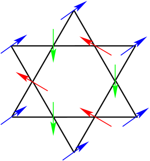
Figure 1: the $\sqrt{3}\times\sqrt{3}$ order.

Figure 2: the $q=0$ order.

Gapped photon phase: When $|J_{xy}|\ll J_{z}<D$, a gapped phase without any symmetry breaking has been found Wen (2003). The low energy excitation with the smallest gap is a loop excitation with the same polarization and gauge symmetry as a photon: the effective theory can be described as a one-component massive compact gauge field.

Plaquette phase: When $|J_{xy}|\ll D$ and $|J_{z}-D|$, $0<D<J_{z}$, a gapped phase with a six-fold degenerate ground state has been found Xu and J.E.Moore (2005). The six-fold degenerate ground state has plaquette order: spins resonate around a subset of the hexagons in the kagome lattice. In this parameter regime, the classical part of this model can be written as

$$H=\sum_{\triangle}\frac{J_{z}}{2}(\sum_{i=1}^{3}S^{z}_{i})^{2}+\sum_{i}(D-J_{z})(S^{z}_{i})^{2}.$$ (2)

When $0<D<J_{z}$, the classical ground states are all the configurations with every triangle occupied by $S^{z}=(1,-1,0)$. Again the classical ground states can be mapped onto the classical 3-color model R.J.Baxter (1970), although the 3-color states correspond to $S^{z}$ instead of spins in the XY plane (Fig. 3).

Figure 3: The classical ground states of (1), when $J_{xy}=0$. Every triangle has configuration $(1,-1,0)$, which can be mapped to the 3 color model on the dual honeycomb lattice.

If small $J_{xy}$ is turned on (either $J_{xy}>0$ or $J_{xy}<0$), the large degeneracy of 3-color ground states is lifted, and the effective Hamiltonian which operates on the low energy Hilbert space is

$$H=\sum_{\hexagon}-t(S^{\dagger}_{1}S^{-}_{2}S^{\dagger}_{3}S^{-}_{4}S^{\dagger}_{5}S^{-}_{6}+H.c.).$$ (3)

1 to 6 are the sites of each hexagon on the kagome lattice. The flippable hexagons have four kinds of configurations, they are $(1,0,1,0,1,0)$ (denoted as $\mathcal{A}_{1}$), $(0,1,0,1,0,1)$ (denoted as $\mathcal{A}_{2}$), $(-1,0,-1,0,-1,0)$ (denoted as $\mathcal{B}_{1}$) and $(0,-1,0,-1,0,-1)$ (denoted as $\mathcal{B}_{2}$). The ring exchange term (3) can flip $\mathcal{A}_{1}$ to $\mathcal{A}_{2}$ (and vice versa) Fig. 4, also can flip $\mathcal{B}_{1}$ to $\mathcal{B}_{2}$ (and vice versa). Two compact $U(1)$ gauge fields were introduced to describe this system, and due to the monopole proliferation, the system is generally gapped, with crystalline order. The particular order which happens here is the plaquette order, which breaks both translational and time-reversal symmetries. The simplest way to view this state is that, since the ring exchange term (3) can flip either $\mathcal{A}_{1}$ to $\mathcal{A}_{2}$ configurations, or flip $\mathcal{B}_{1}$ to $\mathcal{B}_{2}$ configurations, the configurations with the largest number of flippable hexagons are favored in order to benefit from this ring exchange term. Notice that the hexagons form a triangular lattice with three sublattices, then one out of the three sublattices of the triangular lattice can be resonated. Also one can choose either to resonate between $\mathcal{A}_{1}$ and $\mathcal{A}_{2}$ configurations or to resonate between $\mathcal{B}_{1}$ and $\mathcal{B}_{2}$ configurations (these two resonance cannot both happen at the same state). Therefore there are in total $3\times 2=6$ degenerate ground states.

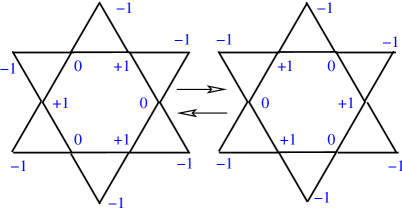
Figure 4: The effect of the ring exchange term (3). It can flip $\mathcal{A}_{1}$ ($\mathcal{B}_{1}$) to $\mathcal{A}_{2}$ ($\mathcal{B}_{2}$), and vice versa.

The simple picture of the ground state will be further justified in the next section, by studying the dual quantum height model. The classical height model was introduced to study the classical 3-color model, and since there are two components of free boson height fields in the continuum limit, it is believed that the low energy field theory should be $c=2$ CFT J.Kondev and C.L.Henley (1996). We will see that the quantum effect is relevant at the classical 3-color critical point, a gap is opened due to the vertex operators of the height fields.

Recently a mean-field treatment of a similar model has been studied Levin and Wen (2006). The plaquette phase we obtained is similar but not entirely identical to the “Plaquette ordered phase” in this recent work, which is identified as the fully packed string crystal. The main difference between the two approaches is that, the monopole effect of compact gauge theory has been taken into account in our work from the very beginning. The monopole effect is supposed to be very relevant at the $z=1$ Gaussian fixed point of gauge theory, and dominate the physics close to the Gaussian fixed point. The nonlocal monopole effects can be described by a local field theory in the dual formalism, and the ordered pattern is predicted in this dual local field theory.

Figure 5: the phase diagram with zero magnetic field. When $D>J_{z}$ and $|J_{xy}|$ is small, the system is in the nondegenerate gapped photon phase; when $0<D<J_{z}$, and with small $|J_{xy}|$, the ground state breaks both translational and time reversal symmetry, resulting in the six-fold degenerate plaquette order; when $J_{xy}$ is negative and large, basically the system is in superfluid order which spontaneously breaks the global spin $S^{z}$ conservation; when $J_{xy}$ is positive and large, $\sqrt{3}\times\sqrt{3}$ order is supposed to be favored; and when $D$ is negative and large, the system has nematic order, with nonzero expectation of $(S^{+})^{2}$.

Nematic phase: When $D<0$ and $|J_{xy}|,J_{z}\ll|D|$, a nematic phase with nonzero expectation value of $(S^{\dagger})^{2}$ has been found Damle and Senthil (2006). In this case, because $D$ is negative and large, the system favors $S^{z}=\pm 1$ on every site. Since the $S^{z}=0$ state costs too much energy, every site can be viewed as an Ising spin, and this model is effectively equivalent to a spin-1/2 model. Since $(S^{-})^{2}$ flips $S^{z}=1$ to $S^{z}=-1$ state, it plays the same role as $\sigma^{-}=\sigma^{x}-i\sigma^{y}$ on the effective Ising spin. Therefore the superfluid phase of this spin-1/2 system is actually the nematic phase of the original spin-1 model.

The rough phase diagram is shown in Fig. 5. The goal of the current work is to understand all the phases we know from the excitations of the six-fold degenerate phase. Basically all the phases can be interpreted as the condensates of various defects which violate the $(1,-1,0)$ constraint in the plaquette phase above. Since the low energy Hilbert space is a constrained one, to create one single defect cannot be realized from local moves of the ground state configurations, instead, global change of all the spins is involved. This implies that one defect in this phase not only carries the global $U(1)$ charge, but also carries the gauge charge, with the gauge symmetry emerged at the low energy constrained Hilbert space. Therefore the condensate of defects is also the Higgs phase of the compact gauge fields.

III Gauge theory of the plaquette-ordered phase

When $J_{xy}=0$ and $0<D<J_{z}$, the set of degenerate ground states can be mapped exactly Xu and J.E.Moore (2005) to those of the 3-color model R.J.Baxter (1970). Every triangle on the kagome lattice has $S^{z}$ configuration $(1,-1,0)$ on this classical critical line. The $z$-component spin configuration on the kagome lattice can be viewed as two-component dimer configurations on the dual honeycomb lattice, with repulsive interaction between two flavors of dimers (every link of the honeycomb lattice can only be occupied by one dimer). It is well-known that the one component quantum dimer model can be mapped to compact gauge theory Fradkin et al. (2004), therefore it is natural to describe this spin-1 system as two compact $U(1)$ gauge fields, since we can interpret the 3-color constraint as two independent $U(1)$ constraints: every site on the honeycomb lattice connects to exactly one $S^{z}=1$ dimer and one $S^{z}=-1$ dimer. We may map the three values of $S^{z}$ to three configurations of a two-component electric field:

$$S^{z}_{i}=0\Rightarrow(E_{1},E_{2})=\frac{1}{\sqrt{3}}(1,0),$$ (4)

$$S^{z}_{i}=1\Rightarrow(E_{1},E_{2})=\frac{1}{\sqrt{3}}(-\frac{1}{2},\frac{\sqrt{3}}{2}),$$ (5)

$$S^{z}_{i}=-1\Rightarrow(E_{1},E_{2})=\frac{1}{\sqrt{3}}(-\frac{1}{2},-\frac{\sqrt{3}}{2}).$$ (6)

Next, note that a 2D unit vector $\hat{\mathbf{n}}_{i}$ can be assigned parallel or antiparallel to each link $i$ of the honeycomb lattice (dual lattice of the kagome lattice) so that vertices of sublattice $A$ of the honeycomb have three incoming bonds, while those of sublattice $B$ have three outgoing bonds. Now define two-component vector fields on bonds: $\vec{E}_{\alpha}=E_{\alpha}\hat{\mathbf{n}}_{i}$. The three color constraint is now equivalent to the Gauss’s law constraint

$$\vec{\nabla}\cdot\vec{E}_{1}=\vec{\nabla}\cdot\vec{E}_{2}=0.$$ (7)

Also we can generalize the configuration of the $E$ vector to a 2d triangular lattice. The lattice is formed by basis $\vec{b}_{1}=(\sqrt{3}/2,1/2)$ and $\vec{b}_{2}=(0,1)$,

$$\vec{E}=n\vec{b}_{1}+m\vec{b}_{2}-(1/(2\sqrt{3}),1/2)$$ (8)

If we add the following interaction to the Hamiltonian, the $\vec{E}$ fields only take three smallest vectors as (6):

$$\frac{1}{\kappa}(\vec{E}_{1}^{2}+\vec{E}_{2}^{2}).$$ (9)

Thus the low energy configurations of electric fields can be one-to-one mapped to the low energy configurations of spins; the spin formalism and the electric field formalism are equivalent.

The perturbation theory of $J_{xy}$ generates a ring exchange (3). The ring-exchange term breaks the $\mathbb{Z}_{3}$ symmetry. Define conjugate operators on each bond $(A_{1,i},A_{2,i})$ with commutation relations

$$[A_{\alpha,j},E_{\beta,k}]=i\delta_{\alpha\beta}\delta_{kj}.$$ (10)

Then operator $T_{\alpha,i}=\exp(iA_{\alpha,j})$ acts as a raising operator: it increases the quantum number $E_{\alpha,j}$ by 1. This enables a compact representation of the ring-exchange terms proportional to $t$: on bond $j$, $\exp(iA_{\alpha,j}l^{(1)}_{\alpha})$ will raise $S^{z}_{j}=0$ to $S^{z}_{j}=1$ if $l^{(1)}=(-\sqrt{3}/2,1/2)$. Similarly, if $l^{(2)}=(-\sqrt{3}/2,-1/2)$ then $\exp(iA_{\alpha,j}l^{(2)}_{\alpha})$ takes $S_{j}^{z}=0$ to $S_{j}^{z}=-1$. Define vector $\vec{A}_{\alpha,j}=A_{\alpha,j}\hat{\mathbf{n}}_{j}$, the ring exchange term around each hexagon becomes

$$H_{ring}=\sum_{i=1}^{2}-t\cos(\vec{\nabla}\times\vec{A}_{\alpha}l^{(i)}_{\alpha}).$$ (11)

Here as usual in gauge theories of lattice spin models, the meaning of $\vec{\nabla}\times\vec{A}$ is that one takes the lattice circulation around a plaquette: for $\hat{v}_{j}$ an clockwise assignment of unit vectors along the links around a hexagon

$$\vec{\nabla}\times\vec{A}=\sum_{j=1}^{6}\hat{v}_{j}\cdot\vec{A}_{j}.$$ (12)

If no defect is present, i.e. the Gauss’s law constraint is strictly imposed, the theory is described by two compact $U(1)$ gauge fields without matter fields. Now let us consider the defects, which are also the gauge charges. When $D$ is much smaller than $J_{z}-D$, the excitation with the smallest gap is to flip one site with $S^{z}=0$ to 1 (or -1), this process actually creates a pair of $(1,1,-1)$ (or $(-1,-1,1)$) defects. Let us denote the density of the $(1,1,-1)$ configuration defect as $\rho_{1}$, and denote the density of the $(1,-1,-1)$ defect as $\rho_{2}$, then from the definition of electric field we can obtain the following relations

$$\vec{\nabla}\cdot\vec{E}_{1}=-\frac{\sqrt{3}}{2}(\rho_{1}+\rho_{2})$$ (13)

$$\vec{\nabla}\cdot\vec{E}_{2}=\frac{1}{2}(\rho_{1}-\rho_{2}).$$ (14)

The charges can be effectively viewed as matter fields defined on the sites of the honeycomb lattice, and the gauge fields $\vec{A}$ and $\vec{E}$ are fields defined on the links of the honeycomb lattice.

For the convenience of later calculations, we need to define a new set of variables as follows

$$\vec{e}_{1}=-\frac{1}{\sqrt{3}}\vec{E}_{1}+\vec{E}_{2}$$ (15)

$$\vec{e}_{2}=-\frac{1}{\sqrt{3}}\vec{E}_{1}-\vec{E}_{2}$$ (16)

$$\vec{a}_{1}=-\frac{\sqrt{3}}{2}\vec{A}_{1}+\frac{1}{2}\vec{A}_{2}$$ (17)

$$\vec{a}_{2}=-\frac{\sqrt{3}}{2}\vec{A}_{1}-\frac{1}{2}\vec{A}_{2}.$$ (18)

Also, one can check that $\vec{e}_{\alpha}$ and $\vec{a}_{\alpha}$ are still conjugate variables :

$$[e_{\alpha,i},a_{\beta,j}]=i\delta_{ij}\delta_{\alpha\beta}.$$ (19)

If the definition for $\vec{e}_{\alpha}$ and $\vec{a}_{\beta}$ is plugged in (14), one can see that $\vec{e}_{\alpha}$ is the electric field corresponding to the charge $\rho_{\alpha}$, in the sense that

$$\vec{\nabla}\cdot\vec{e}_{\alpha}=-\rho_{\alpha}.$$ (20)

When $D$ is smaller than but close to $J_{z}$, $|J_{z}-D|\ll D$, the lowest energy excitation is $(0,0,0)$, and we denote its density as $\rho_{0}$. It carries gauge charge of gauge field $\vec{E}_{1}$

$$\vec{\nabla}\cdot\vec{E}_{1}=\sqrt{3}\rho_{0}=-\frac{\sqrt{3}}{2}(\vec{\nabla}\cdot\vec{e}_{1}+\vec{\nabla}\cdot\vec{e}_{2})$$ (21)

Since the electric fields are subject to the constraint (7), it is convenient to define height fields $\vec{h}$ on the dual triangular lattice.

$$\vec{E}_{\alpha}=(\hat{z}\times\vec{\nabla})h_{\alpha},\vec{\nabla}\times\vec{A}_{\alpha}=\pi_{h\alpha}.$$ (22)

$\pi_{h\alpha}$ and $h_{\alpha}$ are a pair of conjugate variables. The value of $h_{\alpha}$ is also defined on a triangular lattice configuration space, in order to satisfy definition (22), $h_{\alpha}$ is defined in the following way

$$(h_{1},h_{2})_{a}=(\frac{\sqrt{3}}{2}(m+n),\frac{1}{2}(m-n))+(q_{1},q_{2})_{a},$$ (23)

$m$ and $n$ are both integers. Here $a=A,B,C$, denoting the three sublattices on the triangular lattice (dual lattice of the honeycomb lattice). $\vec{q}_{a}$ are three vectors, taking different values on three sublattices

$$\vec{q}_{A}=(\frac{1}{2\sqrt{3}},-\frac{1}{6})$$ (24)

$$\vec{q}_{B}=(-\frac{1}{2\sqrt{3}},-\frac{1}{6})$$ (25)

$$\vec{q}_{C}=(0,\frac{1}{3})$$ (26)

The two-component height variables $h_{\alpha}$ are the same as those introduced in the classical 3-color model (cf. Kondev and Henley J.Kondev and C.L.Henley (1996)). Since $m$ and $n$ are both integers, the vertex operators should enter the effective low energy theory. We will see later that, due to quantum effect, these vertex operators become very relevant and drive the system away from the classical criticality, resulting in a six-fold degenerate plaquette ordered phase. These vertex operators read

$$H_{v}=\sum_{a=A}^{C}-\alpha\cos[2\pi(\frac{1}{\sqrt{3}}h_{1a}+h_{2a}+\frac{1}{\sqrt{3}}q_{1a}+q_{2a})]$$ (27)

$$-\sum_{a=A}^{C}\alpha\cos[2\pi(\frac{1}{\sqrt{3}}h_{1a}-h_{2a}+\frac{1}{\sqrt{3}}q_{1a}-q_{2a})].$$ (28)

For later convenience, we define a new height fields $\phi_{ia}$ and its conjugate variable $\pi_{ia}$ as

$$\phi_{1}=\frac{1}{\sqrt{3}}h_{1}+h_{2}$$ (29)

$$\phi_{2}=\frac{1}{\sqrt{3}}h_{1}-h_{2}$$ (30)

$$\pi_{1}=\frac{\sqrt{3}}{2}\pi_{h1}+\frac{1}{2}\pi_{h2}$$ (31)

$$\pi_{2}=\frac{\sqrt{3}}{2}\pi_{h1}-\frac{1}{2}\pi_{h2}$$ (32)

One can check the commutators and see that $\phi_{\alpha}$ and $\pi_{\alpha}$ are conjugate variables, and based on the definition (18), they are exactly the height fields corresponding to $\vec{e}$ and $\vec{a}$.

$$\vec{e}_{\alpha}=(\hat{z}\times\vec{\nabla})\phi_{\alpha},\vec{\nabla}\times\vec{a}_{\alpha}=\pi_{\alpha}.$$ (33)

The vortex of $\phi_{\alpha}$ is the charge field $\rho_{\alpha}$.

Now in terms of the new height fields, the vertex operators read

$$H_{v}=-\alpha[\cos(2\pi\phi_{1A})+\cos(2\pi\phi_{1B}+\frac{2\pi}{3})$$ (34)

$$+\cos(2\pi\phi_{1C}+\frac{4\pi}{3})$$ (35)

$$+\cos(2\pi\phi_{2A}+\frac{4\pi}{3})+\cos(2\pi\phi_{2B})$$ (36)

$$+\cos(2\pi\phi_{2C}+\frac{2\pi}{3})].$$ (37)

These vertex operators have oscillating signs on the triangular lattice, then in the low energy theory the relevant terms should be higher orders of vertex operators which do not contain oscillating signs on the lattice:

$$H_{v}=-v[\cos(6\pi\varphi_{1})+\cos(6\pi\varphi_{2})]$$ (39)

(40)

$$-v_{1}[\cos(2\pi\varphi_{1}+4\pi\varphi_{2})+\cos(4\pi\varphi_{1}+2\pi\varphi_{2})]$$ (41)

(42)

$$-v_{2}\cos(2\pi\varphi_{1}-2\pi\varphi_{2})+\cdots$$ (43)

$\varphi_{\alpha}$ is the coarse-grained mode of $\phi_{\alpha}$. As the vertex operators correspond to the creation and annihilation of gauge fluxes, the total gauge flux is conserved by mod 3 in the low energy continuum limit. In equation (43), $v$ is supposed to be positive, but $v_{1}$ and $v_{2}$ are supposed to be negative, because when we subtract $\phi_{2}$ from $\phi_{1}$ from (37), it gains angle $2\pi/3$, which generates a factor $-1/2$ before the cosine term in (43). Sine functions of $\varphi_{\alpha}$ are excluded by symmetries of the system. For instance, $\sin(2\pi(\varphi_{1}-\varphi_{2}))$ is excluded by time reversal symmetry.

After coarse-graining the system, the action in terms of $\varphi_{\alpha}$ can be written as

$$L=\sum_{\alpha=1}^{2}(\partial_{\tau}\varphi_{\alpha})^{2}+\rho_{2}(\nabla\varphi_{\alpha})^{2}+H_{v}+\gamma\nabla\varphi_{1}\nabla\varphi_{2}$$ (45)

The $\gamma$ term in (45) is a flavor mixing term between $\varphi_{1}$ and $\varphi_{2}$, and therefore the two flavors of height fields do not only couple to each other through the vertex operators, but also through one of the kinetic terms.

In 2+1d, the potential operators with cosine functions are generally very relevant at the fixed point described by the Gaussian part of the action (45), as long as the $k^{2}$ term ($\rho_{2}$ in (45)) is present. Vertex operators are responsible for the gapped crystalline phases of quantum dimer models, both on the square lattice D.S.Rokhsar and S.A.Kivelson (1988); Fradkin and S.A.Kivelson (1990) and the honeycomb lattice Fradkin et al. (2004). In the current work, the vertex operators are also responsible for the crystalline phases. First of all, let us tune $v_{1}$ and $v_{2}$ to zero, and minimize $v$ terms in (43). Each $\varphi_{\alpha}$ has three minima $0$ , $1/3$, $2/3$. Therefore there are in total 9 different combinations. However, negative $v_{1}$ and $v_{2}$ terms will raise the energy of all the minima with $\varphi_{1}=\varphi_{2}$, and hence we end up with $9-3=6$ minima. This result is actually quite general, for a large parameter regime, there are always 6 minima of the vertex potential in (43). Because the vertex operators in (43) is invariant under transformation $\varphi_{1}\rightarrow\varphi_{1}+1/3$, $\varphi_{2}\rightarrow\varphi_{2}+1/3$, and also invariant under transformation $\varphi_{1}\rightleftarrows\varphi_{2}$, all six minima can be obtained from performing transformations on one single minimum.

Now we can write down the plaquette order parameter in terms of the field theory variables $\varphi_{\alpha}$. The order parameter we are searching for, in the lattice model, is

$$P=\sum_{a=A}^{C}e^{i2\pi(i_{a}-1)/3}(S^{\dagger}_{1a}S^{-}_{2a}S^{\dagger}_{3a}S^{-}_{4a}S^{\dagger}_{5a}S^{-}_{6a}+H.c.)(\sum_{\hexagon}S^{z}_{i})$$ (46)

In the above equation, $a$ represents different sublattices, and $i_{A}=1$, $i_{B}=2$, and $i_{C}=3$. The low energy representation of this order parameter can be deduced from symmetry argument. The most obvious transformations for this order parameter are translational ($\mathrm{T}$) and time reversal ($\mathrm{TR}$) transformations.

$$\mathrm{T}:P\rightarrow e^{i2\pi/3}P,\mathrm{TR}:P\rightarrow-P.$$ (47)

If rotated around hexagons at sublattice $A$ by angle $2\pi/3$ ($\mathrm{R_{2\pi/3}}$), the order parameter is invariant; under space inversion (SI) $\vec{r}\rightarrow-\vec{r}$ and reflection ($\mathrm{P_{x}}$) along $\hat{x}$ ( $y\rightarrow-y$ ) centered at sublattice $A$, the order parameter becomes its complex conjugate

$$\mathrm{SI},\mathrm{P_{x}}:P\rightarrow P^{\ast}.$$ (48)

Under the transformations discussed above, $\varphi_{i}$ transforms as follows:

$$\mathrm{T}:\varphi_{i}\rightarrow\varphi_{i}+\frac{1}{3},$$ (49)

$$\mathrm{TR}:\varphi_{1}\rightleftharpoons\varphi_{2},$$ (50)

$$\mathrm{SI}:\varphi_{\alpha}\rightarrow-\varphi_{\alpha},$$ (51)

$$\mathrm{P_{x}}:\varphi_{\alpha}\rightarrow-\varphi_{\alpha},$$ (52)

$$\mathrm{R_{2\pi/3}}:\varphi_{i}\rightarrow\varphi_{i}.$$ (53)

Summarizing all the transformations above, the field theory representation of the plaquette order parameter $P$ is

$$P\sim(e^{i2\pi\varphi_{2}}-e^{i2\pi\varphi_{1}}).$$ (54)

We can plug in the six minima of the vertex operator (43) to (54), and it gives us 6 different values. All the six expectation values can be obtained by transformation $\langle P_{n}\rangle=\exp(i\pi n/3)\langle P_{0}\rangle$, with $n=1$ to $6$. This implies that the system is in a plaquette order with six fold degeneracy.

When both $v_{1}$ and $v_{2}$ are positive, the vertex operators gives three degenerate minima: $\varphi_{1}=\varphi_{2}=0$, or $\pm 1/3$. These three degenerate ground states do not break time reversal symmetry, but it breaks translational symmetry. The particular order in this case is another type of plaquette order with $(-1,1,-1,1,-1,1)$ hexagons resonating on one of the three sublattices.

The field theory description is only valid when the theory is close to a critical point, i.e. the correlation length is either infinite, or finite but much longer than the microscopic lattice constant. Thus the prediction of plaquette order is only rigorous close to the classical critical point $J_{xy}=0$. But the phase is expected to extend over a finite region in the phase diagram, until a transition into either a disordered phase or one of the other ordered phases derived in the following sections.

In this section we started with mapping the classical ground states of the model onto the classical 3-color model configurations, as in this way we respected the $\mathbb{Z}_{3}$ symmetry of the classical ground state, which is broken by the quantum perturbation. As mentioned before, we can also view the low energy physics of this system as two components of quantum dimer model, with repulsive interaction between two flavors of dimers. From this approach the same low energy action as (45) can be derived. Single component of quantum dimer model generates the kinetic terms and the vertex operator $\cos(6\pi\varphi_{i})$ in (45) at low energy, as discussed in reference Fradkin et al. (2004); the repulsive interaction between the two flavors of dimers will generate the term $\gamma\nabla\varphi_{1}\nabla\varphi_{2}$ and the mixture vertex operators $\cos(2\pi(\varphi_{1}-\varphi_{2}))$ and $\cos(2\pi\varphi_{1}+4\pi\varphi_{2})$, et,al.

IV transition to the featureless gapped photon phase

When $D>J_{z}$, the classical ground state is $S^{z}=0$ on every site, and the low energy excitations are $(+1,-1,+1,-1,....)$ loops. This phase has a single ground state and gapped photon excitations Wen (2003), without any symmetry breaking. In this section we are going to study the phase transition between the six-fold state and the gapped photon phase.

If we start with the six-fold degenerate phase, the transition can be viewed as condensation of $(0,0,0)$ defects. The gap for $(0,0,0)$ defect keeps decreasing as the transition to the gapped photon phase is approached. But the phase boundary between the plaquette phase and the nondegenerate phase is not exactly at $D=J_{z}$ (Fig. 5), this is due to the fact that at second order perturbation of $J_{xy}/J_{z}$, an additional nearest neighbor diagonal interaction is generated. $(0,0,0)$ triangles are more favorable than $(1,-1,0)$ triangles to this diagonal term generated, therefore the second order perturbation effectively increases $D$ by $\sim J_{xy}^{2}/J_{z}$.

The defect $(0,0,0)$ carries charges of both $a_{1\mu}$ and $a_{2\mu}$, and defects at different sublattices of the honeycomb lattice carry opposite gauge charges. If we denote the $(0,0,0)$ defect at sublattice $A$ as $\psi_{A}$ and the $(0,0,0)$ defect at sublattice $B$ as $\psi_{B}$, the effective Lagrangian describing the system close to the transition is

$$L=-t|(\partial_{\mu}-ia_{1\mu}-ia_{2\mu})\psi_{A}|^{2}-t|(\partial_{\mu}+ia_{1\mu}+ia_{2\mu})\psi_{B}|^{2}$$ (55)

(56)

Notice that the $(0,0,0)$ defect carries zero global $U(1)$ charge (a $(0,0,0)$ defect does not carry any $S^{z}$), and therefore one $\psi_{A}$ particle and one $\psi_{B}$ particles can be annihilated together, so the term $g(\psi_{A}\psi_{B}+H.c.)$ is allowed in the interaction. After the condensation of $\psi_{A}$ and $\psi_{B}$, the gauge field $a_{+\mu}=a_{1\mu}+a_{2\mu}$ will be gapped out along with the phase mode $\theta_{A}-\theta_{B}$, and the mode $\theta_{A}+\theta_{B}$ will be gapped out by the interaction $g(\psi_{A}\psi_{B}+H.c.)$ ($\theta_{A}$ and $\theta_{B}$ are phase angles of $\psi_{A}$ and $\psi_{B}$ respectively). Therefore in the condensate there is no gapless excitation, which is consistent with the gapped photon phase.

To further justify this picture, let us first take a Landau-Ginzburg tour to study this transition. Let us define complex field $\Phi$ to describe the low energy mode of the plaquette order parameter $P$. The LG action for this transition is as follows

$$L=|\partial_{\mu}\Phi|^{2}-r|\Phi|^{2}+u(|\Phi|^{2})^{2}+g(\Phi^{6}+H.c.).$$ (57)

Without the $g$ term, the theory describes an 3D XY transition. The $g$ term turns on an $\mathbb{Z}_{6}$ anisotropy at this critical point. In the ordered state of $\Phi$, this anisotropy is a relevant perturbation and will lead to a six-fold degeneracy. At the $3D$ XY critical point, $\mathbb{Z}_{6}$ anisotropy is irrelevant, thus the Landau-Ginzburg theory predicts that the transition between the six-fold states and the featureless gapped photon phase is a 3D XY transition.

The 3D XY transition is driven by the vortices of $\Phi$, and after the condensation of the vortices, the vortex core state grows and becomes the macroscopic order. It has been shown before that the vortex core of the height field of the quantum dimer model is an unpaired spin, which implies that the condensate of vortices breaks the spin $SU(2)$ symmetry spontaneously (for instance, the Neel state). In our case, the vortex configuration of $\Phi$ (including the core) has been depicted in Fig. 6. Around every vortex core, there are 6 domains separated by domain walls, each domain is one state out of the six-fold degenerate plaquette ordered states. In the ordered phase, the vortices are linearly confined due to the pinning potential $\Phi^{6}+H.c.$, because the domain walls would cost energy proportional to their length. At the critical point since the pinning potential is irrelevant, the vortices are deconfined.

In Fig. 6, one can see that the vortex core is actually a (0,0,0) triangle, which is the lowest energy defect when $D\sim J_{z}$. If the height field representation of $\Phi$ (54) is taken, one can see that the vortex of $\Phi$ is a bound state of one vortex of $\varphi_{1}$ and one vortex of $\varphi_{2}$. Thus a vortex of $\Phi$ carries one gauge charge of $a_{1\mu}$ and one gauge charge of $a_{2\mu}$, i.e. this vortex carries the same gauge charge as the $(0,0,0)$ defect. Therefore indeed the transition between the six-fold plaquette state and the featureless photon phase is driven by the $(0,0,0)$ defects.

The dual field theory of (57) would describe the vortex condensation directly. After the standard superfluid-gauge field duality in 2+1d, the dual theory reads

$$L=-t|(\partial_{\mu}-iA_{\mu})\psi|^{2}+\cdots$$ (58)

Herein $\psi$ is the vortex creation operator, and the $\mathbb{Z}_{6}$ anisotropy term in (57) becomes the monopole processes which annihilate and create the fluxes of gauge field $A_{\mu}$. By comparing equation (58) and equation (56), we can see that $A_{\mu}=a_{1\mu}+a_{2\mu}$, and $\psi=\psi_{A}=\psi_{B}^{\dagger}$. Please note that because $\psi_{A}$ and $\psi_{B}$ can annihilate together, there is actually only one flavor of defect, and $\psi_{B}=\psi_{A}^{\dagger}$. In the ordered phase the gauge field $A_{\mu}$ is gapped out by monopole proliferation, and $\psi$ is confined; in the nondegenerate photon phase the gauge field is gapped out with $\psi$ through the Higgs mechanism. The gauge field is only gapless at the critical point.

Figure 6: The vortex and vortex core configuration in the six-fold plaquette order. Every vortex is surrounded by six phase domains and 6 domain walls, the vortex core is exactly a $(0,0,0)$ defect. In this figure, $\mathrm{B+}$ denotes resonating $(1,0,1,0,1,0)$ plaquette on sublattice $\mathrm{B}$. The six domains around this vortex core are (count counterclockwise): $A+$ with $\Phi\sim\Phi_{0}$, and $\vec{\varphi}=\vec{\varphi}_{0}+(1/3,2/3)$; $C-$ with $\Phi\sim\exp(i\pi/3)\Phi_{0}$ and $\vec{\varphi}=\vec{\varphi}_{0}+(1/3,0)$, $B+$ with $\Phi\sim\exp(i2\pi/3)\Phi_{0}$ and $\vec{\varphi}=\vec{\varphi}_{0}+(2/3,0)$; $A-$ with $\Phi\sim\exp(i\pi)\Phi_{0}$ and $\vec{\varphi}=\vec{\varphi}_{0}+(2/3,1/3)$; $C+$ with $\Phi\sim\exp(i4\pi/3)\Phi_{0}$ and $\vec{\varphi}=\vec{\varphi}_{0}+(0,1/3)$, $B-$ with $\Phi\sim\exp(i5\pi/3)\Phi_{0}$ and $\vec{\varphi}=\vec{\varphi}_{0}+(0,2/3)$. The arrows show the circulation of the phase of $\Phi$. Also, this vortex is a bound state of one vortex of $\varphi_{1}$ and one vortex of $\varphi_{2}$. The spins are defined on the links of the honeycomb lattice, which are the sites of the kagome lattice. links with + and - are occupied by spin states $S^{z}=+1$ and $-1$. The red dashed lines denote the domain walls.

If we plug in the height field representation of $\Phi$ in equation (54) into the LG action (57), it reproduces the height field action in equation (45), thus the phase transition between the gapped photon phase and the plaquette phase can also be studied in the dual height model. We define new height fields $\varphi_{\pm}=(\varphi_{1}\pm\varphi_{2})/2$, and they satisfy the following relation

$$(\vec{e}_{1}\pm\vec{e}_{2})/2=(\hat{z}\times\vec{\nabla})\varphi_{\pm}.$$ (59)

Now the height field Lagrangian reads

$$L=t(\partial_{\tau}\varphi_{+})^{2}+\rho_{2}(\nabla\varphi_{+})^{2}+t^{\prime}(\partial_{\tau}\varphi_{-})^{2}+\rho^{\prime}_{2}(\nabla\varphi_{-})^{2}$$ (60)

(61)

$$-v\cos(6\pi\varphi_{+})\cos(6\pi\varphi_{-})-v_{1}\cos(6\pi\varphi_{+})\cos(2\pi\varphi_{-})$$ (62)

(63)

$$-v_{2}\cos(4\pi\varphi_{-}).$$ (64)

One $(0,0,0)$ defect carries one unit gauge charge of $(e_{1}+e_{2})/2$, thus it is one unit vortex of $\varphi_{+}$, and the condensation of $(0,0,0)$ drives $\varphi_{+}$ into disordered phase. In the condensate, $\varphi_{+}$ is disordered and the expectation value of $\cos(2\pi\varphi_{+})$ is zero. Thus the plaquette order parameter

$$P \sim e^{i2\pi\varphi_{2}}-e^{i2\pi\varphi_{1}}\sim i\sin(2\pi\varphi_{-})\exp(i2\pi\varphi_{+})$$ (65)

takes zero expectation value: the plaquette order disappears. Since $\varphi_{-}$ does not transform under translation or rotation by $2\pi/3$ transformations, any crystalline pattern which breaks these symmetries cannot exist.

When field $\varphi_{+}$ is disordered, the ordered pattern and symmetry of the ground state can be studied from the effective action for height field $\varphi_{-}$, which remains gapped and ordered. Thus the order of the condensate is determined by the series of vertex operators of $\varphi_{-}$, since the leading vertex operator is $-v_{2}\cos(4\pi\varphi_{-})$, for a large range of parameters, the minima are at $\varphi_{-}=\pm 1/4$. However, let us imagine writing down a physical order parameter which only involves $\varphi_{-}=(\varphi_{1}-\varphi_{2})/2$, since any physical order parameter should be invariant under transformation $\varphi_{\alpha}\rightarrow\varphi_{\alpha}+1$, this order parameter should be invariant under $\varphi_{-}\rightarrow\varphi_{-}+1/2$, thus the ground states $\varphi_{-}=\pm 1/4$ are physically equivalent to each other, and the ground state is nondegenerate, which is again consistent with the gapped photon phase.

At the transition, since only $\varphi_{-}$ is ordered, we can plug in the minimum of $\varphi_{-}$ into (64), and obtain an effective action for $\varphi_{+}$. Notice that both $v$ and $v_{1}$ vertex operators vanish after plugging in the minima $\varphi_{-}=1/4$. The leading operator that survives is $\cos(12\pi\varphi_{+})$, which is a $\mathbb{Z}_{6}$ anisotropy. The height field theory which describes this transition is

$$L=(\partial_{\mu}\varphi_{+})^{2}-\alpha\cos(12\pi\varphi_{+}).$$ (66)

This action describes an XY transition as the $\mathbb{Z}_{6}$ anisotropy term is irrelevant at the XY critical point. Thus we conclude that the transition between the six-fold state and the featureless photon phase is driven by the condensation of $(0,0,0)$ defect, and the critical point belongs to the 3D XY universality class.

V transition to the superfluid state

When $J_{xy}$ is negative and large, the system is in the superfluid phase (ferromagnetic phase in spin XY plane), with nonzero expectation value of $\langle S^{\dagger}\rangle$. In this section we are going to study the transition between the six-fold degenerate plaquette phase and the superfluid phase. Let us first focus on the region where $D\ll|J_{z}-D|$; in this parameter regime, the defects with the lowest gap are $(1,1,-1)$ and $(1,-1,-1)$ triangles. It was shown in section III that these two defects are vortices of $\varphi_{1}$ and $\varphi_{2}$ respectively. As an example, a vortex of height field $\varphi_{1}$ is shown in Fig. 7, one can see that the core of this vortex is a $(1,1,-1)$ defect. When the vortices of the height fields condense, which means the height fields are disordered, the system enters a superfluid phase. When $D$ and $J_{xy}$ are small, the phase transition occurs when the hopping energy of the defects is comparable with the gap, the phase boundary is roughly $D\sim J_{xy}$, as shown in the phase diagram Fig. 5.

Figure 7: The vortex and vortex core configuration of $\varphi_{1}$. Every vortex is surrounded by 3 phase domains and 3 domain walls, the vortex core is exactly a $(1,1,-1)$ defect. The three domains around this vortex core are (count counterclockwise): $B+$ with $\vec{\varphi}=\vec{\varphi}_{0}+(2/3,0)$; $B-$ with $\vec{\varphi}=\vec{\varphi}_{0}+(0,2/3)$, $A+$ with $\vec{\varphi}=\vec{\varphi}_{0}+(1/3,0)$. The arrows show the circulation of $\varphi_{1}$.

Defect $(1,1,-1)$ can stay at two sublattices of the honeycomb lattice, let us denote defect $(1,1,-1)$ at sublattice $A$ as $\psi_{1A}$, denote defect $(1,1,-1)$ at sublattice $B$ as $\psi_{1B}$; denote defect $(1,-1,-1)$ at sublattice $A$ as $\psi_{2A}$, defect $(1,-1,-1)$ at sublattice $B$ as $\psi_{2B}$. Herein 4 flavors of defects are defined because these defects have independent conservation laws instead of just one global $U(1)$ conservation law in the original Hamiltonian. If we want to hop one $(1,1,-1)$ defect from sublattice $A$ to sublattice $B$, global spin configurations within the low energy subspace should be changed; this means that any local operator cannot hop $(1,1,-1)$ defect from sublattice $A$ to $B$, i.e. defects at sublattice $A$ and $B$ are separately conserved. This situation is similar to the doped quantum dimer model on square lattice Balents et al. (2005a), in that case the doped holes can also only hop in one sublattice due to the gauge symmetry of the dimer model. The gauge symmetry of the dimer model is due to the dimer constraint imposed automatically.

According to equation (20), $\psi_{1A}$ ($\psi_{1B}$) carries charge $+1$ (-1) of gauge field $a_{1\mu}$, and $\psi_{2A}$ ($\psi_{2B}$) carries charge $+1$ (-1) of gauge field $a_{2\mu}$. Now the effective Lagrangian describing the system is

$$L=-t|(\partial_{\mu}-ia_{1\mu})\psi_{1A}|^{2}-t|(\partial_{\mu}+ia_{1\mu})\psi_{1B}|^{2}$$ (67)

(68)

$$-t|(\partial_{\mu}-ia_{2\mu})\psi_{2A}|^{2}-t|(\partial_{\mu}+ia_{2\mu})\psi_{2B}|^{2}$$ (69)

(70)

$$+\cdots\cdots.$$ (71)

The ellipses include the monopoles of gauge fields as well as the interaction terms between different matter fields. The interaction has to be consistent with all the internal symmetries of the system, which is $U(1)_{global}\times U(1)_{gauge}\times U(1)_{gauge}$. The $U(1)$ gauge symmetries correspond to the two flavors of gauge fields, and the $U(1)$ global symmetry corresponds to the conservation of $S^{z}$. The regular terms like $-r|\psi_{ia}|^{2}+O(|\psi|^{4})$ are all allowed, besides these terms, another term should in principle exist, which is $-g(\psi_{1A}\psi_{1B}\psi_{2A}\psi_{2B}+H.c.)$. Four different flavors of particles can be created and annihilated together, without any global reconfigurations.

The superfluid phase can be viewed as the condensate of 4 flavors of matter fields. Let us denote $\psi_{ia}\sim\exp(\theta_{ia})$, the action can be written as

$$L=-\tilde{t}(\partial_{\mu}\theta_{1A}-a_{1\mu})^{2}-\tilde{t}(\partial_{\mu}\theta_{1B}+a_{1\mu})^{2}$$ (72)

(73)

$$-\tilde{t}(\partial_{\mu}\theta_{2A}-a_{2\mu})^{2}-\tilde{t}(\partial_{\mu}\theta_{2B}+a_{2\mu})^{2}$$ (74)

(75)

$$+g\cos(\theta_{1A}+\theta_{1B}+\theta_{2A}+\theta_{2B}).$$ (76)

If there is no gauge field, the condensation of $\theta$s would lead to four gapless Goldstone modes. However, in the condensate, mode $\theta_{1A}+\theta_{1B}+\theta_{2A}+\theta_{2B}$ is gapped out by the $g$ term in (76), this implies that in the superfluid phase $\theta_{1A}+\theta_{1B}=-(\theta_{2A}+\theta_{2B})$. Meanwhile, $\theta_{1A}-\theta_{1B}$ will gap out $a_{1\mu}$ through the Higgs mechanism, $\theta_{2A}-\theta_{2B}$ will also gap out $a_{2\mu}$ through the Higgs mechanism, therefore the only gapless mode in the condensate is $\theta_{1A}+\theta_{1B}$ = $-(\theta_{2A}+\theta_{2B})$.

Notice that $S^{\dagger}_{i}$ can create a pair of $\psi_{1A}$ and $\psi_{1B}$ particles and also can annihilate a pair of $\psi_{2A}$ and $\psi_{2B}$ particles. Therefore we can identify

$$S^{\dagger}\sim\exp[i(\theta_{1A}+\theta_{1B})]=\exp[-i(\theta_{2A}+\theta_{2B})].$$ (77)

Thus, the Goldstone mode $\theta_{1A}+\theta_{1B}$ is exactly the global $U(1)$ phason mode of $S^{\dagger}\sim\exp(i\theta)$.

If one approaches the transition from the superfluid phase, the transition can be viewed as condensation of vortices in the superfluid. There are four components of vortices, corresponding to the four flavors of matter fields. The gapless Goldstone mode becomes the noncompact $U(1)$ gauge field in the dual language. The vertex operators in the height field language are the vortex tunnelling terms. The vertex operators create or annihilate gauge flux of the original gauge fields $a_{1\mu}$ and $a_{2\mu}$. For instance, $\exp(2\pi i\varphi_{1})$ creates one unit flux of $a_{1\mu}$. As pointed out in references Balents et al. (2005a, b), when one flavor of gauge field is coupled to two different matter fields, the vortex of each matter field carries half flux quantum. Since vortex $v_{1A}$ and $v_{1B}$ carry opposite gauge flux, the vertex operator $\cos(6\pi\varphi_{1})$ corresponds to tunnelling process $v_{1A}^{\dagger 3}v_{1B}^{3}+H.c.$. The dual Lagrangian can be effectively written as

$$L=-t|(\partial_{\mu}-iA_{\mu})v_{1A}|^{2}-t|(\partial_{\mu}-iA_{\mu})v_{1B}|^{2}$$ (78)

(79)

$$-t|(\partial_{\mu}+iA_{\mu})v_{2A}|^{2}-t|(\partial_{\mu}+iA_{\mu})v_{2B}|^{2}$$ (80)

(81)

$$+g(v_{1A}^{\dagger 3}v_{1B}^{3}+H.c.)+g(v_{2A}^{\dagger 3}v_{2B}^{3}+H.c.)$$ (82)

(83)

$$+g_{2}(v^{\dagger}_{1A}v_{1B}v^{\dagger}_{2B}v_{2A}+H.c.)+\eta(v_{1A}v_{1B}v_{2B}v_{2A}+H.c.)$$ (84)

(85)

$$+g_{1}(v^{\dagger}_{1A}v_{1B}v^{\dagger 2}_{2A}v^{2}_{2B}+H.c.)+g_{1}(v^{\dagger}_{2A}v_{2B}v^{\dagger 2}_{1A}v^{2}_{1B}+H.c.)$$ (86)

(87)

$A_{\mu}$ in (87) is the dual form of the Goldstone “phason” mode in the superfluid phase. $g$, $g_{1}$ and $g_{2}$ are the tunnelling terms due to the vertex operators in (43). Tunnelling term $\eta$ is independent of monopoles, as this term conserves the total vorticity (consistent with the $U(1)$ gauge symmetry of (87)), and also conserves the total gauge flux of the gauge fields $a_{1\mu}$ and $a_{2\mu}$, therefore it should exist in the field theory.

Let us denote $v_{ia}\sim\exp(-i\chi_{ia})$. After the condensation of vortices, modes $\chi_{1A}-\chi_{1B}$ and $\chi_{2A}-\chi_{2B}$ are gapped out by the monopoles. Mode $\chi_{1A}+\chi_{1B}+\chi_{2A}+\chi_{2B}$ are gapped out by the $\gamma$ term in equation (87), i.e. $\chi_{1A}+\chi_{1B}=-(\chi_{2A}+\chi_{2B})$; also $\chi_{1A}+\chi_{1B}$ is gapped out by $A_{\mu}$ through the Higgs mechanism. Therefore in the condensate of vortices, there is no gapless excitations, which is consistent with the crystalline phase.

If the monopole effect is turned off, the transition point is described by two gapless noncompact gauge fields and four flavors of matter fields. However, whether these gapless gauge fields and matter fields can survive when the monopoles are turned on is an open question. If the monopoles gap out the gauge field and confine the matter fields, at the transition there is no gapless excitation. In this case our theory predicts a direct first order transition.

The superfluid phase and the plaquette phase break different symmetries, and according to the classic Landau phase transition theory, the transition should be either first order, or split into two transitions, with a disordered phase (or a phase with both orders) in between. There is no universal law that guarantees one direct first order transition.

In our theory, the intermediate phases can be understood as the condensate of composites of defect $\psi_{ia}$. A gapped disordered phase can be obtained if composites which only carry local gauge charges but no global $U(1)$ charge are condensed. For instance, if composites $\psi_{1A}^{\dagger}\psi_{1B}$ and $\psi_{2A}^{\dagger}\psi_{2B}$ are condensed while all the other composites are disordered, the gauge fields are gapped through the Higgs mechanism, therefore the height fields are disordered, the crystalline order disappears. Also, since the composites carry zero global $U(1)$ charge, there is no gapless Goldstone mode. Thus we can conclude that the condensate of $\psi_{1A}^{\dagger}\psi_{1B}$ and $\psi_{2A}^{\dagger}\psi_{2B}$ is a spin disordered phase i.e. a spin liquid phase. Notice that $\psi_{1A}^{\dagger}\psi_{1B}$ ($\psi_{2A}^{\dagger}\psi_{2B}$) carries two unit gauge charges of gauge field $a_{1\mu}$ ($a_{2\mu}$), therefore the condensate of $\psi_{1A}^{\dagger}\psi_{1B}$ and $\psi_{2A}^{\dagger}\psi_{2B}$ is a spin liquid with $\mathbb{Z}_{2}\times\mathbb{Z}_{2}$ gauge symmetry, which is the residual gauge symmetry after the condensation of the composites of matter fields. On the other hand, if composites carrying only global $U(1)$ charge are condensed, the superfluid order should coexist with the crystalline order. For instance, the composite $\psi_{1A}^{\dagger}\psi_{1B}^{\dagger}\psi_{2A}\psi_{2B}$ does not carry any gauge charge, the condensate of this composite is a superfluid order, and the crystalline order still exists. Thus this phase is a supersolid phase.

VI transition to the nematic phase

The existence of nematic phase can be derived easily at the negative large $D$ limit. When $D$ is negative and becomes the dominant term in the Hamiltonian (1), the system is effectively a spin-1/2 system, since $S^{z}$ on each site can only be $\pm 1$. The classical ground state of this model is that every unit triangle should have either $(1,1,-1)$ or $(1,-1,-1)$ configuration. This classical ground state is the same as the classical Ising model on the kagome lattice, with large degeneracy. If the same Boltzman weight is imposed for each classical ground state, the kagome lattice Ising model is disordered, and the correlation length is finite R.Moessner and S.L.Sondhi (2001). By contrast, a related classical system is the classical Ising model on the triangular lattice, while if the same Boltzman weight is imposed for each classical ground state, the triangular lattice Ising model is critical, and an infinitesimal quantum perturbation is relevant at this critical point and drive the system into a crystalline phase. If infinitesimal transverse magnetic field $h\sigma^{x}$ is turned on, the system is driven to $\sqrt{3}\times\sqrt{3}$ order R.Moessner and S.L.Sondhi (2001); if ferromagnetic $XY$ exchange $-J_{xy}(\sigma^{x}_{i}\sigma^{x}_{j}+\sigma^{y}_{i}\sigma^{y}_{j})$ is turned on, the system is driven into a supersolid phase, which breaks both $U(1)$ symmetry ( $\langle\sigma^{+}\rangle\neq 0$ ), and translational symmetry Melko et al. (2005). Unlike the Ising model on the triangular lattice, the classical Ising model on the kagome lattice is disordered, with finite correlation length. In the original Hamiltonian (1), if $|J_{xy}|\ll D$, the second order perturbation generates a term which flips $S^{z}=1$ state to $S^{z}=-1$ state and vice versa. The effective Hamiltonian reads

$$H_{eff}=\sum_{<i,j>}-t(\sigma^{x}_{i}\sigma^{x}_{j}+\sigma^{y}_{i}\sigma^{y}_{j})+J_{z}\sigma^{z}_{i}\sigma^{z}_{j}.$$ (88)

$t\sim J_{xy}^{2}/D$. As studied in Melko et al. (2005); Damle and Senthil (2006), for the spin-1/2 system on the kagome lattice, infinitesimal ferromagnetic $XY$ exchange yields superfluid order, $\langle\sigma^{\dagger}\rangle\neq 0$. The spin-1/2 raising operator is the nematic order parameter $(S^{+})^{2}$, therefore infinitesimal $|J_{xy}|$ drives the system into a nematic phase.

Although the nematic phase and the plaquette phase do not necessarily touch each other in the phase diagram, a direct transition between these two phases is possible when they are adjacent in the phase diagram. It is conceivable that a certain type of spin Hamiltonian can realize the direct transition between the nematic phase and the six-fold plaquette phase. This direct transition is more likely to occur when $J_{xy}>0$ than the case with $J_{xy}<0$. In the case with $J_{xy}>0$, every hexagon is effectively penetrated by one $\pi$ flux of $a_{1\mu}$ and one $\pi$ flux of $a_{2\mu}$. The motion of defects is strongly affected by the background magnetic fields, and several interesting possibilities can happen. One of the possibilities is that the defects condense in pairs, i.e. $\langle(\psi_{ia})^{2}\rangle\neq 0$, as a pair of defects does not see any background flux. After the pair condensation, the Goldstone mode is $2(\theta_{1A}+\theta_{1B})$, corresponding to the phase of $(S^{\dagger})^{2}$, so the system is in the nematic phase discussed above Damle and Senthil (2006). One important difference between the nematic phase and the superfluid phase is that, each vortex in the nematic phase only carries one quarter flux of the gauge fields, therefore the vertex terms in (43) correspond to even higher order of vortex tunnelling processes.

A direct transition between the nematic phase and the plaquette phase can be described by the following action of paired matter field $\Psi_{ia}=(\psi_{ia})^{2}$

$$L=-t|(\partial_{\mu}-2ia_{1\mu})\Psi_{1A}|^{2}-t|(\partial_{\mu}+2ia_{1\mu})\Psi_{1B}|^{2}$$ (89)

(90)

$$-t|(\partial_{\mu}-2ia_{2\mu})\Psi_{2A}|^{2}-t|(\partial_{\mu}+2ia_{2\mu})\Psi_{2B}|^{2}$$ (91)

(92)

$$-H_{I}+\cdots\cdots.$$ (93)

Again the ellipses include the monopole terms, and $H_{I}$ contains all the possible interaction terms between matter fields. Just like the four-defect creation term discussed in the previous section, $g\Psi_{1A}\Psi_{1B}\Psi_{2A}\Psi_{2B}+H.c.$ should in principle exist in the interaction, thus phason mode $\sum_{i=1}^{2}\sum_{a=A}^{B}\theta_{ia}$ is gapped out in the condensate of $\Psi_{ia}$. Without the monopole terms this transition is a gapless second order transition.

Now the question boils down to if the monopole effect is going to be relevant at the critical point described by action (93). Since the nematic phase is a pair condensate, each single vortex in the nematic phase carries only one quarter flux of each flavor of gauge fields, so the vertex operator in (43) corresponds to even higher order of tunnelling processes than the superfluid case. The dual action now reads

$$L=-t|(\partial_{\mu}-iA_{\mu})v_{1A}|^{2}-t|(\partial_{\mu}-iA_{\mu})v_{1B}|^{2}$$ (94)

(95)

$$-t|(\partial_{\mu}+iA_{\mu})v_{2A}|^{2}-t|(\partial_{\mu}+iA_{\mu})v_{2B}|^{2}$$ (96)

(97)

(98)

$$+g(v_{1A}^{\dagger 6}v_{1B}^{6}+H.c.)+g(v_{2A}^{\dagger 6}v_{2B}^{6}+H.c.)$$ (99)

(100)

$$+g^{\prime}(v^{\dagger 2}_{1A}v^{2}_{1B}v^{\dagger 2}_{2B}v^{2}_{2A}+H.c.)+\eta(v_{1A}v_{1B}v_{2B}v_{2A}+H.c.)$$ (101)

(102)

$$g_{1}(v^{\dagger 2}_{1A}v^{2}_{1B}v^{\dagger 4}_{2A}v^{4}_{2B}+H.c.)+g_{1}(v^{\dagger 2}_{2A}v^{2}_{2B}v^{\dagger 4}_{1A}v^{4}_{1B}+H.c.)$$ (103)

$g$, $g_{1}$ and $g_{2}$ terms are vortex tunnelling processes corresponding to the vertex operators in (43), notice that now $v_{1A}$ and $v_{1B}$ ($v_{2A}$ and $v_{2B}$) carry one quarter unit flux of $a_{1\mu}$ ($a_{2\mu}$) . $\eta$ term is a tunnelling which does not rely on monopole, as it not only complies with the $U(1)$ gauge symmetry of the dual action (103), but also conserves the flux numbers of the original gauge fields $a_{1\mu}$ and $a_{2\mu}$. Following the similar argument as references Senthil et al. (2004a, b), the monopole terms (vortex tunnelling terms) are likely (but not rigorously proved) irrelevant at the transition fixed point. It is known that at the 3D $XY$ fixed point, $\mathbb{Z}_{4}$ anisotropy is irrelevant, while the $\mathbb{Z}_{3}$ anisotropy as in (43) could be relevant. However in our case, the vertex operators in (43) could be irrelevant at the transition due to the pairing of gauge charges (93). Although the vertex operators are always relevant at the Gaussian fixed point of (45), it could be irrelevant at the order-disorder transition of height fields. It is expected, as in the calculation that follows, that the scaling dimension of the vertex operators is approximately proportional to the number of flavors of matter fields, and proportional to the square of the product of electric charge and magnetic charge Murthy and Sachdev (1990).

We can roughly estimate the scaling dimension of the monopole operators from a random phase approximation (RPA) calculation. After integrating out the Gaussian part of the matter fields in (93), an effective action for gauge fields $a_{1\mu}$ and $a_{2\mu}$ is generated

$$L=\sum_{\alpha=1}^{2}\int\frac{d^{3}k}{(2\pi)^{3}}Nn^{2}|k|\sigma_{0}|\vec{a}(k)_{\alpha}|^{2}+\cdots\cdots.$$ (105)

$N$ is the number of flavors of bosons coupled to each gauge field, $n$ is the number of gauge charge carried by each boson. In our case $N=n=2$. In the dual theory, the kinetic term for the height field is softened to be $\sim k^{3}$, and the monopole energy diverges logarithmically instead of converging in the infrared limit Kleinert et al. (2002); Herbut and Seradjeh (2003). The dual height fields now have the action

$$L=\sum_{\alpha=1}^{2}\int\frac{d^{3}k}{(2\pi)^{3}}\frac{k^{3}}{Nn^{2}\sigma_{0}}|\varphi_{\alpha}|^{2}-H_{v}.$$ (106)

From this calculation one can see that the scaling dimension of vertex operators is proportional to $Nn^{2}$.

$H_{v}$ in (43) contains three types of terms. The scaling dimensions for $\cos(6\pi\varphi_{\alpha})$ and $\cos(2\pi\varphi_{1}+4\pi\varphi_{2})$ calculated from the RPA approximation is higher than the $\mathbb{Z}_{4}$ anisotropy studied before Senthil et al. (2004a, b). The third vertex operator is $\cos(2\pi(\varphi_{1}-\varphi_{2}))$, the scaling dimension calculated from RPA is higher than the $\mathbb{Z}_{3}$ anisotropy of 3D $XY$ fixed point, also, on the RPA level, the scaling dimension is equal to the case with $\mathbb{Z}_{4}$ anisotropy and $N=1$ discussed in reference Senthil et al. (2004b), which has been shown to be irrelevant at the transition between the Higgs phase and the confined phase. Recently a Monte Carlo simulation has shown that the transition between the crystalline phase and the superfluid phase in a bosonic model with 1/3 filling on the kagome lattice is a very weak first order transition Isakov et al. (2006), on the RPA level, the scaling dimension of the monopole in that case is smaller than the dimension of all the triple vertices and very close to the scaling dimension of $\cos(2\pi(\varphi_{1}-\varphi_{2}))$ in our case. Therefore it is possible that the vertex operators in our problem are irrelevant at the transition between the nematic phase and the plaquette order. When the vertex operators are irrelevant, the critical point is a direct gapless second order transition, with four flavors of deconfined matter fields, as well as two flavors of noncompact gauge fields.

VII transition to the $\sqrt{3}\times\sqrt{3}$ phase

When $J_{xy}>0$ and much larger than other coefficients, the state is most likely to be either the $\sqrt{3}\times\sqrt{3}$ order in Fig. 1, or the $q=0$ state in Fig. 2. From the $1/S$ expansion, this $\sqrt{3}\times\sqrt{3}$ order is supposed to be the global minimum of all the classical degenerate ground states of the Heisenberg model on the kagome lattice at the isotropic point C.L.Henley and E.P.Chan (1995), although the $q=0$ state has also been proved to be one of the local minima. Both $\sqrt{3}\times\sqrt{3}$ and $q=0$ states are very typical configurations for spins on kagome, they can be stabilized by the second or third nearest neighbor interactions. Also, since both states are coplanar, they are expected to be even better candidates in the large $J_{xy}$ case.

Since now the defect hopping is frustrated by the background magnetic flux of gauge field $a_{1\mu}$ and $a_{2\mu}$ through each hexagon, the phase angle of the defects cannot be uniformly distributed on the whole lattice. We will see that the $\sqrt{3}\times\sqrt{3}$ phase can be interpreted as the condensate of the four flavors of charge fields in the background gauge fluxes.

Because of the interaction between different matter fields $g(\psi_{1A}\psi_{1B}\psi_{2A}\psi_{2B}+H.c.)$, we have the following relation between the phase angles

$$\theta=\theta_{1A}+\theta_{1B}=-(\theta_{2A}+\theta_{2B}),$$ (107)

$\theta$ is the phase angle of $S^{-}$. The distribution of phase $\theta$ can be deduced from the distribution of $\theta_{1A}$ and $\theta_{1B}$. Notice that $\psi_{1A}$ and $\psi_{1B}$ both live on the sites of the honeycomb lattice, and hop on two different triangular sublattices (Fig. 8). With a background magnetic field $a_{1\mu}$, the effective Hamiltonian for the motion of $\psi_{1A}$ is

$$H=\sum_{<i,j>}t\cos(\theta_{1A,i}-\theta_{1A,j})+\cdots\cdots$$ (108)

This is an antiferromagnetic $XY$ model on the triangular lattice, and after the condensation of $\theta_{1A}$, the ground state is the $\sqrt{3}\times\sqrt{3}$ order. This phase can be viewed as the staggered vortex density phase on the triangular lattice.

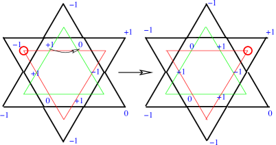
Figure 8: Defects which violate the 3-color constraint hop on one of the two triangular sublattices (red and green) of the honeycomb lattice.

If both $\psi_{1A}$ and $\psi_{1B}$ condense (due to the time reversal symmetry, if $\psi_{1A}$ and $\psi_{1B}$ condense, $\psi_{2A}$ and $\psi_{2B}$ will also condense), the phase angle $\theta$ can be determined from the distribution of $\theta_{1A}$ and $\theta_{1B}$. By adding the two ordered patterns of both $\theta_{1A}$ and $\theta_{1B}$ together, the ordered pattern for $\theta$ is automatically obtained, and the order can only be either $q=0$ state or the $\sqrt{3}\times\sqrt{3}$ state (Fig. 9) and (Fig. 10). In these ordered phases, the Goldstone mode is still $\theta=\theta_{1A}+\theta_{1B}$.

Figure 9: The $\sqrt{3}\times\sqrt{3}$ order of $\theta$ obtained from the ordered pattern of $\theta_{1A}$ and $\theta_{1B}$. The black arrow corresponds to angle $\theta$, and the pattern of $\theta$ can be obtained from its adjacent red arrow ($\theta_{1A}$) and green arrow ($\theta_{1B}$).

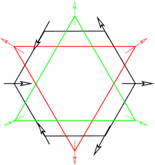
Figure 10: $q=0$ order of $\theta$ obtained from ordered pattern of $\theta_{1A}$ and $\theta_{1B}$.

VIII longitudinal magnetic field

A longitudinal magnetic field along $\hat{z}$ breaks the time reversal symmetry in the Hamiltonian, and much of the physics is significantly changed. Let us assume the magnetic field is small, i.e. $hS^{z}$ is much smaller than $J_{z}$ and $D$ in the model. Note that this precludes accessing strong-field phenomena such as magnetization plateaus in this theory.

The six-fold degenerate plaquette phase is expected to survive in a small longitudinal magnetic field. Since in a small magnetic field, the classical ground states without $J_{xy}$ are still configurations with $(1,-1,0)$ triangles only, and therefore the ring exchange term generated by $J_{xy}$ is still going to select the plaquette ordered state as the ground state.

However, the excitation energies of defects are changed by the longitudinal field: $(1,1,-1)$ defects have lower gap than the $(1,-1,-1)$ defects. Therefore when $|J_{xy}|$ is turned on, $(1,1,-1)$ defects should condense before $(1,-1,-1)$. As we will see in this section, the condensate of $(1,1,-1)$ defect is actually a supersolid phase, with both global $U(1)$ symmetry breaking and the space symmetry breaking.

Let us take the case with $J_{xy}<0$ as an example. As long as $(1,-1,-1)$ defects remain confined and gapped, the total number of $(1,1,-1)$ defects is conserved before its condensing, because $(1,1,-1)$ defects cannot be excited without $(1,-1,-1)$ defects due to the conservation of total $S^{z}$. Therefore when $(1,1,-1)$ defects condense and $(1,-1,-1)$ defects remain confined and gapped, the system still has a gapless Goldstone mode due to the spontaneous breaking of the global conservation of $(1,1,-1)$ defects. The gapless Goldstone mode manifests the superfluid phase.

Secondly, the spatial symmetry breaking can still be studied in terms of the dual height fields. Because $(1,1,-1)$ is the vortex of height field $\varphi_{1}$, the condensate of $(1,1,-1)$ charge is the disordered phase of $\varphi_{1}$, $\varphi_{1}$ no longer has nonzero expectation values. However, because $\varphi_{2}$ is still ordered, the vertex operator $-\alpha\cos(6\pi\varphi_{2})$ in (43) has 3 minima, corresponding to 3 fold degenerate states. These 3 minima are the plaquette orders of $(-1,0,-1,0,-1,0)$ hexagon on 3 different sublattices.

The height fields $\varphi_{1}$ and $\varphi_{2}$ are coupled through the vertex operators as shown in (43). This coupling is not going to lift the 3 fold degeneracy of $\varphi_{2}$ when $\varphi_{1}$ is disordered. The reason is as follows: The whole action (45) is invariant under transformation $\varphi_{1}\rightarrow\varphi_{1}+1/3$, $\varphi_{2}\rightarrow\varphi_{2}+1/3$. Since $\varphi_{1}$ is disordered, after integrating over $\varphi_{1}$, the effective action $H_{eff}(\varphi_{2})$ for $\varphi_{2}$ does not break this symmetry, and the leading vertex term generated from integrating out $\varphi_{1}$ is $\cos(6\pi\varphi_{2})$. This can be clearly seen from the following equations

$$\exp(-H_{eff}(\varphi_{2}))=\int D\varphi_{1}\exp(-H(\varphi_{1},\varphi_{2}))$$ (109)

(110)

$$=\int D\varphi_{1}\exp(-H(\varphi_{1}+1/3,\varphi_{2}+1/3))=$$ (111)

(112)

$$\int D(\varphi_{1}+1/3)\exp(-H(\varphi_{1}+1/3,\varphi_{2}+1/3))$$ (113)

(114)

$$=\int D\varphi_{1}\exp(-H(\varphi_{1},\varphi_{2}+1/3))$$ (115)

(116)

$$=\exp(-H_{eff}(\varphi_{2}+1/3)).$$ (117)

Notice that the above proof is only valid if $\varphi_{1}$ does not take any nonzero expectation value, i.e. $\varphi_{1}$ is in disordered phase. Alternatively, one can understand this argument from the conservation of the gauge fluxes. Vertex operator $\cos(2\pi\varphi_{\alpha})$ can annihilate or create one unit flux of gauge field $a_{\alpha\mu}$. The total flux of both gauge fields is conserved mod 3 in vertex operator Hamiltonian (43), and as the disordered phase of $\varphi_{1}$ (the condensate of $(1,1,-1)$ defect) does not tend to violate this conservation, the resultant effective Hamiltonian after integrating out $\varphi_{1}$ fields does not break the $\mathbb{Z}_{3}$ conservation of total gauge flux, i.e. the lowest order vertex operator of the resultant effective Hamiltonian of $\varphi_{2}$ is $\cos(6\pi\varphi_{2})$. Therefore the 3-fold degenerate plaquette order is not lifted. A similar result is obtained for $J_{xy}>0$ too. Thus, the phase with defect $(1,1,-1)$ condensed while defect $(1,-1,-1)$ confined breaks both spatial symmetry and the global $U(1)$ symmetry, and hence must be the supersolid phase.

When $D<0$ and large, a small longitudinal magnetic field changes the physics severely. In this regime, the classical ground state has Ising configuration $(1,1,-1)$ on each triangle. In the previous sections we mentioned that the classical Ising ground state on the kagome lattice is disordered with finite correlation length. However, once the longitudinal magnetic field is turned on, every triangle has $(1,1,-1)$ configuration. Since the sites of the kagome lattice are the links of the dual honeycomb lattice, the ground state configurations with small magnetic field can be mapped onto the dimer configurations on the honeycomb lattice, with $S^{z}=-1$ mapped onto dimer, and $S^{z}=1$ mapped onto empty link. If the same Boltzmann weight is imposed on every dimer configuration, the system is again critical, with power law decaying spin-spin correlation function.

Since the classical ground state is critical, it is again very instable against quantum perturbations. If a small $J_{xy}$ is turned on, the system is driven into a gapped crystalline phase. At the sixth-order perturbation, a ring exchange term is generated

$$H_{ring}=\sum_{\hexagon}-t((S^{\dagger}_{1}S_{2})^{2}(S^{\dagger}_{3}S_{4})^{2}(S^{\dagger}_{5}S_{6})^{2}+H.c.)$$ (118)

$t\sim J^{6}_{xy}/(J_{z}^{2}D^{3})$. This ring exchange term plays the same role as the dimer flipping term in the honeycomb lattice quantum dimer model, which will generally lead to a crystalline phase. Notice that, besides the off-diagonal flipping term in (118), diagonal terms are also generated. According to several previous works Bergman et al. (2006a, b), the diagonal terms generated by perturbation theory favor flippable hexagons, therefore it is expected that the crystalline order is either plaquette order or columnar order Moessner et al. (2003).

Figure 11: The distribution of $S^{z}=1$ and $S^{z}=-1$ sites on the kagome lattice is equivalent to the distribution of dimers of dimer model on the dual honeycomb lattice. The ring exchange term (118) plays the same role as the dimer resonating term in the quantum dimer model.

Presumably the crystalline phase disappears when $J_{xy}^{2}/D\sim h$, Since the sign of $t$ in (118) is always positive (independent of the sign of $J_{xy}$), the crystalline phase should extends symmetrically on the two sides of the classical line with $J_{xy}=0$, until the system enters the nematic phase. The sketchy phase diagram in a small magnetic field is shown in Fig. 12, note that this phase diagram involves a lot of phases, the detailed topology of the phase diagram would depend on the details of the microscopic model.

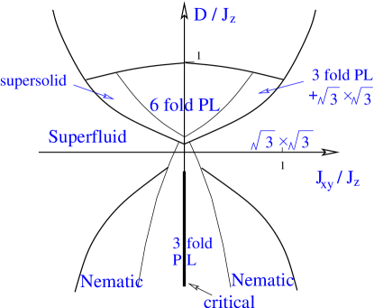
Figure 12: The phase diagram in small longitudinal magnetic field $h$. The difference between this phase diagram and the one without magnetic field in Fig. 5 is that, between the plaquette phase and the superfluid phase there is a supersolid phase. And in the negative and large $D$ case, small $J_{xy}$ is going to generate a gapped crystalline order.

IX the $SU(2)$ point

At the isotropic point $J_{xy}=J_{z}$ and $D=0$, the $\sqrt{3}\times\sqrt{3}$ state is just one possibility. This state is obtained from quantum perturbation on the classical limit. If we start with the quantum limit, another possible state can be obtained: the $q=0$ dimer plaquette state.

This state can be understood quite easily from the quantum dimer model on the kagome lattice. For a spin-1 system, each site can form two spin singlets, which means each site connects to two dimers. Since every site on the kagome lattice is shared by four links, this dimer model is half filled. The dimer resonance term on the kagome lattice is shown in Fig. 13, which can flip the dimer covering $\mathcal{C}_{1}$ to $\mathcal{C}_{2}$ and vice versa. The dimer model Hamiltonian is now written as

$$H=-t(|\mathcal{C}_{1}\rangle\langle\mathcal{C}_{2}|+H.c.)+V(|\mathcal{C}_{1}\rangle\langle\mathcal{C}_{1}|+|\mathcal{C}_{2}\rangle\langle\mathcal{C}_{2}|).$$ (119)

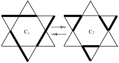
Figure 13: The dimer model on the kagome lattice. Since this is a spin-1 system, every site connects to two dimers. The dimer flipping term flips configuration $\mathcal{C}_{1}$ to $\mathcal{C}_{2}$ and vice versa.

As long as $V<t$, the exact ground state wave function of this Hamiltonian can be written as

$$|\Psi\rangle=\frac{1}{Z}\prod_{\hexagon}(|\mathcal{C}_{1}\rangle+|\mathcal{C}_{2}\rangle).$$ (120)

This state does not break any space symmetry, and it minimizes the energy of each hexagon individually. This state should be the ground state of a certain type $SU(2)$ invariant spin Hamiltonian.

Now the question is whether this dimer plaquette phase is a new phase or it can be continuously connected with one of the other states discussed early this paper without any physical singularity. Notice that the gapped photon phase with $(0,0,0)$ on every triangle breaks no space symmetry either, thus one can imagine adding $D(S^{z})^{2}$ on the isotropic Hamiltonian, and the ground state wave function can be continuously deformed to the gapped photon phase.

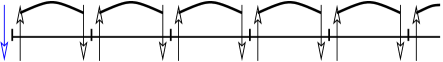
Figure 14: A typical state in the Haldane phase. In the bulk, every site is shared by two dimers. However, at each edge, there is one residual unpaired spin-1/2 variable.

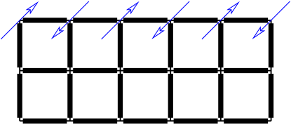
Figure 15: The edge of AKLT state on the square lattice. There is one extra spin-1/2 degree of freedom on each site of the edge, therefore the edge state is effectively a spin-1/2 spin chain, which is either gapless or breaks translational symmetry. The AKLT state is qualitatively different from the state with $S^{z}=0$ everywhere.

Figure 16: The edge of the kagome lattice. Every unit cell at the edge has even number of spin-1/2 quantities. Presumably the edge state is gapped and featureless.

One has to be careful about the naive argument above. Let us consider the one dimensional analogues of the dimer plaquette phase and the (0,0,0) phase as a check of our naive argument. The one dimensional Haldane phase Haldane (1988) for spin-1 Heisenberg chain is gapped, and breaks no symmetry. One can imagine that by adding $D(S^{z})^{2}$ on the Heisenberg Hamiltonian the Haldane phase will be continuously connected to the state with $S^{z}=0$ everywhere. However, the spin-1 Heisenberg chain is characterized by two special properties: the first is the existence of gapless edge states, the second is the hidden diluted antiferromagnetic order. The existence of the gapless edge states can be understood as follows: All the sites in the bulk are shared by two dimers, while the site at the edge only connects to one dimer, hence there is a residual spin-1/2 degree of freedom at each edge (Fig. 14). The hidden diluted antiferromagnetic order can be viewed from expanding the AKLT state (the explicit wavefunction of one particular state in the Haldane phase) of the spin-1 chain in the basis of $S^{z}$. In this expansion, one typical state is as follows

$$+-00000+000-+00-+000\cdots\cdots$$ (121)

Every $S^{z}=1$ site is always followed by one $S^{z}=-1$ site, although there could be a number of $S^{z}=0$ sites in between. A special nonlocal string operator could be introduced to describe this hidden order in the Haldane phase den Nijs and Rommelse (1987, 1989).

The nice features of the Haldane phase also exist in the AKLT state of spin-2 systems on the square lattice. Let us take a cylinder geometry as an example. There is one unpaired spin-1/2 degree of freedom on each site of the edge, therefore the edge state is effectively a spin-1/2 chain, which is either gapless or gapped but breaks translational symmetry. The AKLT state is qualitatively different from the state with $S^{z}=0$ everywhere as well (Fig. 15).

However, the edge states are missing in the dimer plaquette phase of the spin-1 dimer model on the kagome lattice. If we take a cylinder with edges, on each site of the edge there is also a residual spin-1/2 degree of freedom. However, due to the geometry of the kagome lattice, in every unit cell of the edge there are even number of spins, therefore effectively the edge state is a chain with integer spin (Fig. 16). The resultant edge state is generally gapped and featureless at the edge, which is the Haldane phase on a closed circle. Thus, we conclude that the dimer plaquette phase can be continuously connected with the gapped photon phase, with $(0,0,0)$ spin configuration on every triangle.

X Other transitions

In the phase diagrams Fig. 5 and Fig. 12, there are several other transitions which are interesting. First of all, in Fig. 5, the transition between the nematic phase and the superfluid phase is probably an Ising transition, as this transition breaks the $\mathbb{Z}_{2}$ symmetry in the nematic state. The transition between the nematic phase and the $\sqrt{3}\times\sqrt{3}$ phase is supposed to be a first order transition.

In the case with magnetic field, since another crystalline order is opened up (Fig. 12), there is a transition between the crystalline phase and the nematic phase. However, now that in the case of large and negative $D$, the system can be described by an effective spin-1/2 model (88), the transition can be understood as the transition between the crystalline order and the superfluid order of hard core bosons on the kagome lattice. This transition has been studied in references Isakov et al. (2006); Sengupta et al. (2006), and the transition is a weak first order transition.

XI conclusions and extensions

In the current work we studied the global phase diagram of the spin-1 XXZ antiferromagnet on the kagome lattice. Various phases which have been studied before can be obtained from condensation of the defects in one single phase. The phase diagram was also obtained for the case of a magnetic field along the $z$ direction. One route to test this phase diagram experimentally is by neutron scattering or other measurements on the spin-1 kagome materials, for instance $\mathrm{Ni_{3}V_{2}O_{8}}$ and $\mathrm{BF_{4}}$ salts.

In all the previous sections, the model under consideration only contains quadratic interactions. However, in some circumstances, for instance a spin-1 bosonic system trapped in an optical lattice, the biquadratic interactions $-J_{2}(\vec{S}_{1}\cdot\vec{S}_{2})^{2}$ have been shown to be important Imambekov et al. (2003). This biquadratic term can help to stabilize the nematic phase, when it becomes the dominant term in the Hamiltonian. In closing we briefly explain one interesting consequence of this biquadratic interaction, in case a cold-atom realization of this Hamiltonian is constructed.

Suppose that the system is in the six-fold degenerate plaquette ordered state, and let us gradually turn on the biquadratic term in the XY plane

$$H_{bi}=-J_{2}(S^{x}_{i}S^{x}_{j}+S^{y}_{i}S^{y}_{j})^{2}.$$ (122)

This biquadratic term is consistent with the $XXZ$ symmetry of our model. At the third order in perturbation theory, this biquadratic term can generate resonance between $(+1,-1,+1,-1,+1,-1)$ hexagon with $(-1,+1,-1,+1,-1,+1)$. Notice that, although spin $S^{z}=+1$, $-1$ and $0$ are treated as three colors, the $\mathbb{Z}_{3}$ symmetry is missing in Hamiltonian (11), since the resonances were only between $(+1,0,+1,0,+1,0)$ hexagons and between the $(-1,0,-1,0,-1,0)$ hexagons. Therefore the full $\mathbb{Z}_{3}$ symmetry can be restored by turning on the biquadratic term (122). At this $\mathbb{Z}_{3}$ point the ground state is probably a nine-fold degenerate plaquette order. Once the biquadratic XY exchange dominates the quadratic XY exchange, the phase becomes a three-fold degenerate plaquette ordered state with resonating $(+1,-1)$ hexagons.