Slave bosons in radial gauge: a bridge between path integral and hamiltonian language

Abstract

We establish a correspondence between the resummation of world lines and the diagonalization of the Hamiltonian for a strongly correlated electronic system. For this purpose, we analyze the functional integrals for the partition function and the correlation functions invoking a slave boson representation in the radial gauge. We show in the spinless case that the Green’s function of the physical electron and the projected Green’s function of the pseudofermion coincide. Correlation and Green’s functions in the spinful case involve a complex entanglement of the world lines which, however, can be obtained through a strikingly simple extension of the spinless scheme. As a toy model we investigate the two-site cluster of the single impurity Anderson model which yields analytical results. All expectation values and dynamical correlation functions are obtained from the exact calculation of the relevant functional integrals. The hole density, the hole auto-correlation function and the Green’s function are computed, and a comparison between spinless and spin 1/2 systems provides insight into the role of the radial slave boson field. In particular, the exact expectation value of the radial slave boson field is finite in both cases, and it is not related to a Bose condensate.

, ,

1 Introduction

In contemporary solid state research, strongly correlated electrons comprise the most fascinating albeit intangible physical systems. They cover a wide range of phenomena, including high temperature superconductivity, colossal magnetoresistance, aspects of the fractional quantum Hall effect, and even electronic reconstruction in oxide electronic devices which are built on interfaces of strongly correlated films. Whereas their importance is generally perceived, a fundamental comprehension is still not achieved, especially for high-temperature superconductivity.

This unfortunate absence of a well established theoretical scheme or even solution is not surprising: strong electronic correlations are based on (sufficiently strong) local interactions in real space but the Fermi surface, the concept on which the physics of metals is firmly rooted, is defined and understood in momentum space. Correspondingly, a theoretical investigation is either built on momentum or real space approaches which allow to treat either the kinetic (band) term or the interaction accurately. However, a momentum-space weak coupling approach is insufficient to generate the desired new energy scales and fix points whereas standard perturbation theory from the highly degenerate local (atomic) limit suffers from severe drawbacks Pai00 .

Nevertheless, many effective strong coupling theories expand, in a generalized sense, with respect to local models. A model with a single local interaction term is the Anderson impurity model. It is the prominent strong-coupling many-body model which can still be solved exactly (with certain restrictions) and which has been understood in basically all aspects (see, for example Anderson70 ; Nozieres74 ; Wilson75 ; Andrei80 ; Wiegmann80 ). It may justly be seen as the paradigm of a strongly correlated many-body system. A successful scheme to investigate lattice models with on-site interactions originates from a self-consistent extension of the Anderson model. The self-consistency is generated through a dynamical mean-field theory (DMFT) which singles out a site with strong local interaction; this site couples to an electronic bath, the effective medium, the local density of states of which is calculated self-consistently Georges92 ; Georges96 . Actually, the DMFT is exact for infinite space dimensions, a limit which was introduced in Ref. Metzner89 for correlated electron systems. However, it is missing the spatial correlations. In recent years it has been devised to treat clusters which can couple to various bath systems in order to investigate correlations with a spatial extension of the cluster size Maier05 ; cdmft ; bk ; Potthoff05 ; Kyung06 .

In our theoretical study we will focus on a different approach, the slave boson technique BAR76 ; Col84 ; KOT86 . The formalism entails a local decomposition of electronic excitations into charge and spin components. Electron creation and annihilation operators are thereby represented by composite operators which separate into canonical operators with bosonic and fermionic character. However these operators are enslaved in the sense that their respective number operators have to fulfill a local constraint. The original idea was to decouple spin and charge degrees of freedom; other, modified schemes attribute to each type of excitation a bosonic mode which allows to study the correlated system in a saddle point approximation KOT86 ; FRE92 ; Has97 . This mean field approach has been successful when set against numerical simulations: ground state energies Fre91 and charge structure factors show excellent agreement Zimmermann97 , as the procedure is exact in the large degeneracy limit FRE92 ; Flo02 .

While the saddle point approximation allows to calculate translationally invariant expectation values in momentum space, the corresponding mean field solution is not a priori legitimate. The objection is concerned with the local decomposition of the electron field into fermion and slave boson components. This implies that the model acquires a local gauge invariance with the consequence that Elitzur’s theorem Elitzur75 prevents the (slave) bosonic fields to acquire a non-zero expectation value. In fact, it is the phase fluctuations of the boson field which suppress the finite value or condensation of these fields.

One alternative to avoid such a condensation has been devised by Kroha, Wölfle, and coworkers Kroha97 ; Kirchner04 . In their approach the local gauge invariance is guaranteed through Ward identities in a conserving approximation. The projection onto the physical sector of the Fock space is achieved with an Abrikosov procedure by sending the Lagrange multiplier of the constraint to infinity. The other alternative is to use a radial decomposition of the bosonic field Read , the details of which were presented in a previous paper by two of the authors FRE01 . In the limit of large on-site interaction, the bosonic fields in radial representation reduce to their respective (real) amplitude as the time derivatives of the conjugate phase can be absorbed in a time-dependent Lagrange multiplier field.

In this article we provide a scheme for the solution of cluster models in radial slave-boson representation. We present in sufficient detail the calculation of correlation and Green’s functions for a two-site cluster of the single impurity Anderson model, in order to exemplify our scheme. Although the model can be diagonalized without slave boson technique we esteem the explicit solution in the radial decomposition of considerable significance. First, it relates the world line expansion of slave boson path integrals to the quantum states in the Fock space, in particular for entangled states. This is achieved through a decomposition of the fermionic determinant into resolvents at each time step. Second, it allows to compare these exact results (e. g., for the slave boson amplitude) to saddle point evaluations and to assess their validity OUE07 .

The article is organized as follows: in Sec. 2, we introduce the functional integral formulation of the two-site cluster model. We give expressions for the action, partition function and hole density as well as for the hole autocorrelation function in terms of radial slave bosons. The spinless system is studied first in Sec. 3 where, through the derivation of the partition function, we show how to proceed from a world line representation to the representation with quantum states in the Fock space. In Sec. 4, we show how our formalism allows to derive results for the spinful case from a straightforward extension of the spinless case. The Green’s function necessitates a distinct derivation of the fundamental connection between the slave-boson path integral representation and the hamiltonian scheme which is the object of Sec. 5.

2 Functional integral formulation of the two-site cluster model

2.1 Hamiltonian and radial slave boson representation

The single impurity Anderson model (SIAM) has been investigated with a variety of techniques and for many different purposes. One of them consists of testing a new approach, in particular against exact results. Here we adopt a similar spirit in order to link the evaluation of the path integral representation of thermodynamic and dynamical quantities to their computation through a straightforward diagonalization of the Hamiltonian. For the SIAM it reads:

$${\mathcal{H}}=\sum_{k,\sigma}c^{\dagger}_{k,\sigma}(t^{\phantom{\dagger}}_{k}+\epsilon_{\rm c})c^{\phantom{\dagger}}_{k,\sigma}+\sum_{\sigma}d^{\dagger}_{\sigma}\epsilon_{\rm d}d^{\phantom{\dagger}}_{\sigma}+V\sum_{k,\sigma}\left(c^{\dagger}_{k,\sigma}d^{\phantom{\dagger}}_{\sigma}+{\rm h.c.}\right)+U\prod_{\sigma=\uparrow,\downarrow}d^{\dagger}_{\sigma}d^{\phantom{\dagger}}_{\sigma},$$ (1)

where $U$ is the on-site repulsion, which is hereafter taken as infinite. The operators $c^{\dagger}_{k,\sigma}$ ($c^{\phantom{\dagger}}_{k,\sigma}$) and $d^{\dagger}_{\sigma}$ ($d^{\phantom{\dagger}}_{\sigma}$) describe the creation (annihilation) of the band electrons and impurity electrons respectively, with spin $\sigma$; the kinetic energy in the band is denoted $t^{\phantom{\dagger}}_{k}$, and $\epsilon_{\rm c}$ and $\epsilon_{\rm d}$ are the band and impurity energy levels, respectively. The hybridization is given by $V$.

The link between the two schemes is actually a complex procedure when the impurity is coupled to an infinite bath. In order to lower this complexity we reduce the bath to a single site, in which case the diagonalization of the Hamiltonian is easy and all relevant results can be obtained analytically. Nevertheless, the problem is non-trivial when handled in the functional integral formalism. The level of difficulty depends on the functional representation which is used. For our purpose, a promising one is that of the slave boson (SB) representation in the radial gauge FRE01 . It is based on the original representation by Barnes BAR76 and is augmented in that respect that the underlying $U(1)$ gauge symmetry, originally discussed by Read and Newns Read , is fully implemented, as the phase of the bosonic field is integrated out from the outset. Accordingly, the original field $d^{\phantom{\dagger}}_{\sigma}$ is represented in terms of a real and a Grassmann field for each spin:

$$d^{\phantom{\dagger}}_{n,\sigma} = x^{\phantom{\dagger}}_{n+1}f^{\phantom{\dagger}}_{n,\sigma}$$ (2)

$$d^{\dagger}_{n,\sigma} = x^{\phantom{\dagger}}_{n}f^{\dagger}_{n,\sigma},$$ (3)

where $x^{\phantom{\dagger}}_{n}$ and $x^{\phantom{\dagger}}_{n+1}$ are the slave boson field amplitudes at time steps $n$ and $n+1$, and $f^{\phantom{\dagger}}_{n,\sigma}$ is the auxiliary fermion field. The shift of one time step for $x$ in the relation for $d^{\phantom{\dagger}}_{n,\sigma}$ is necessary to obtain a non-zero value of the Grassmann integration for the Green’s functions $-\langle d^{\phantom{\dagger}}_{\sigma}(\tau)d^{{\dagger}}_{\sigma}(0)\rangle$ as clearly shown for its calculation in the atomic limit in Ref. FRE01 . More precisely, the path integral is zero if $x^{\phantom{\dagger}}_{n+1}$ is replaced by $x^{\phantom{\dagger}}_{n}$ in Eq. (2). Moreover, Eqs. (2) and (3) are required in order to properly represent the hybridization term in the action as given below. Further detail on this matter can be found in Ref. FRE01 .

2.2 Action and partition function

Following Ref. FRE01 , the path integral representation of the partition function of the two-site cluster is given by:

$${\mathcal{Z}}=\lim_{\begin{subarray}{c}N\rightarrow\infty\\ W\rightarrow\infty\end{subarray}}\left(\prod_{n=1}^{N}\int\prod_{\sigma}D[f_{n,\sigma},f^{\dagger}_{n,\sigma}]D[c_{n,\sigma},c^{\dagger}_{n,\sigma}]\int_{-\infty}^{\infty}\frac{\displaystyle\delta{\rm d}\lambda_{n}}{\displaystyle 2\pi}\int_{-\infty}^{\infty}{\rm d}x_{n}\right)e^{-S}$$ (4)

where the action $S$ may be written as the sum of a fermionic part, $S_{f}$, and a bosonic part, $S_{b}$, with

$$S_{f} = \sum_{\sigma}S_{f,\sigma}=\sum_{n=1}^{N}\sum_{\sigma}\left[c^{\dagger}_{n,\sigma}(c_{n,\sigma}-L_{\rm c}c_{n-1,\sigma})+f^{\dagger}_{n,\sigma}(f_{n,\sigma}-L_{n}f_{n-1,\sigma})\right.$$

$$~{}~{}~{}~{}~{}~{}~{}~{}~{}~{}~{}~{}~{}~{}~{}~{}~{}~{}~{}~{}~{}~{}~{}\left.+V\delta x_{n}(c^{\dagger}_{n,\sigma}f_{n-1,\sigma}+f^{\dagger}_{n,\sigma}c_{n-1,\sigma})\right]$$

$$S_{b} = \sum_{n=1}^{N}\left[\delta\left(i\lambda_{n}(x_{n}-1)+Wx_{n}(x_{n}-1)\right)\right],$$

where $L_{\rm c}=e^{-\delta(\epsilon_{\rm c}-\mu)}$, $L_{n}=e^{-\delta(\epsilon_{\rm d}-\mu+i\lambda_{n})}\equiv L_{\rm d}~{}e^{-i\delta\lambda_{n}}$, $\lambda_{n}$ is the time-dependent real constraint field, $n$ denotes the time steps, and $\delta\equiv\beta/N$, with $\beta=1/k_{\rm B}T$ and $N$ the number of time steps. Here, $S_{f}$ ($S_{f,\sigma}$) is bilinear in the fermionic fields, and the corresponding matrix of the coefficients will be denoted as $\left[S\right]$ ($\left[S_{0}\right]$). The positive real number $W$ is sent to infinity at the end of the calculation which guarantees the projection onto the physical subspace. The above treatment of the bosonic field is specific to radial slave bosons: no phase variable appears, and the above form cannot be obtained by transformations of the conventional functional integral in the Cartesian gauge without further assumptions (see Ref. FRE01 ).

Inserting Eq. (2.2) into Eq. (4) yields a particularly suggestive expression of the partition function ${\mathcal{Z}}$ in the functional integral formulation, of the kind:

$${\mathcal{Z}}=\lim_{\begin{subarray}{c}N\rightarrow\infty\\ W\rightarrow\infty\end{subarray}}{\mathcal{P}_{1}}\ldots{\mathcal{P}_{N}}~{}\mbox{det}\left[S\right],$$ (6)

where det$\left[S\right]$ is the determinant of the fermionic matrix defined by Eq. (2.2); ${\mathcal{P}}_{n}$ is defined as:

$${\mathcal{P}}_{n}=\int_{-\infty}^{+\infty}\delta~{}\frac{\displaystyle{\rm d}\lambda_{n}}{\displaystyle 2\pi}~{}\int_{-\infty}^{+\infty}{\rm d}x_{n}~{}e^{-\delta\left[i\lambda_{n}(x_{n}-1)+Wx_{n}(x_{n}-1)\right]},$$ (7)

and acts as a projector from the enlarged Fock space “spanned” by the auxiliary fermionic fields down to the physical one. Explicitly, the action of these projectors on the various contributions resulting from $\mbox{det}\left[S\right]$ are found to be:

$${\mathcal{P}}_{n}\cdot 1 = 1,$$ (8)

$${\mathcal{P}}_{n}\cdot x_{n} = 1,$$ (9)

$${\mathcal{P}}_{n}\cdot L_{\rm n} = L_{d},$$ (10)

$${\mathcal{P}}_{n}\cdot L_{n}x_{n} = 0,$$ (11)

$${\mathcal{P}}_{n}\cdot L_{n}^{2} = 0,$$ (12)

$${\mathcal{P}}_{n}\cdot x_{n}^{2} = 1.$$ (13)

As will be seen below no further property of ${\mathcal{P}}_{n}$ will be needed for our purpose. We note that there is some freedom in writing the projectors ${\mathcal{P}}_{n}$, and alternative expressions exist FRE01 . However the properties Eqs. (8)–(13) are independent of the particular form of ${\mathcal{P}}_{n}$.

3 Application to the spinless fermion case

We first consider a spinless fermion system for simplicity. Even though this is a non-interacting problem, the level of complexity of its path integral representation following from Eqs. (4)–(6), is equivalent to the one of a fully interacting problem. The matrix representation of the action $S_{f,\sigma}$ of such system is a $2N\times 2N$ square matrix whose explicit expression in the basis $\{c_{n,\sigma},f_{n,\sigma}\}$ reads:

$$\left[S_{0}\right]=\left(\begin{array}[]{cccc}1\mbox{I}_{2}&{}\hfil&{}\hfil&-\left[{\mathcal{L}}_{1}\right]\\ \left[{\mathcal{L}}_{2}\right]&1\mbox{I}_{2}&{}\hfil&{}\hfil\\ {}\hfil&\ddots&\ddots&{}\hfil\\ {}\hfil&{}\hfil&\left[{\mathcal{L}}_{\rm N}\right]&1\mbox{I}_{2}\end{array}\right),$$ (18)

where $1\mbox{I}_{2}$ is the 2$\times$2 identity matrix and $\left[{\mathcal{L}}_{n}\right]$ are 2$\times$2 blocks given by:

$$\left[{\mathcal{L}}_{n}\right]=\left(\begin{array}[]{cc}-L_{\rm c}&\delta Vx_{n}\\ \delta Vx_{n}&-L_{n}\end{array}\right),$$ (21)

at time step $n$, $1\leq n\leq N$. Note that the matrix $\left[S_{0}\right]$ as defined in Eq. (18) has the same structure as the action matrix $S^{(\alpha)}$ in Chap. 2 of Ref. NEG88 .

3.1 Partition function

The partition function ${\mathcal{Z}}_{0}$ of the spinless fermion system has a form similar to that of Eq. (6) except that $\mbox{det}\left[S\right]$ is replaced by $\mbox{det}\left[S_{0}\right]$. Its calculation is straightforward since we only have to evaluate:

$${\mathcal{Z}}_{0}=\lim_{\begin{subarray}{c}N\rightarrow\infty\\ W\rightarrow\infty\end{subarray}}{\mathcal{P}_{1}}\ldots{\mathcal{P}_{N}}~{}\sum_{\{P\}}\mbox{sgn}(P)\prod_{n=1}^{2N}S_{P(n),n}$$ (22)

where $\mbox{sgn}(P)$ is the signum function of permutations $P$ in the permutation group ${\mathcal{S}}_{2N}$ and $S_{i,j}$ are the matrix elements of $\left[S_{0}\right]$. Since the time step $n$ is only involved in $S_{i,2n-3}$ and $S_{i,2n-2}$ we may recast Eq. (22) into:

$${\mathcal{Z}}_{0} = \lim_{\begin{subarray}{c}N\rightarrow\infty\\ W\rightarrow\infty\end{subarray}}\sum_{\{P\}}\mbox{sgn}(P)~{}{\mathcal{P}}_{2}\left(S_{P(1),1}S_{P(2),2}\right)\ldots$$ (23)

$$\times {\mathcal{P}}_{N}\left(S_{P(2N-3),2N-3}S_{P(2N-2),2N-2}\right){\mathcal{P}}_{1}\left(S_{P(2N-1),2N-1}S_{P(2N),2N}\right).$$

At this point it is straightforward to verify that performing the projections only implies to make use of Eqs. (8)–(10). We are left with:

$${\mathcal{Z}}_{0}=\lim_{N\rightarrow\infty}~{}\sum_{\{P\}}\mbox{sgn}(P)\prod_{n=1}^{2N}S_{P(n),n}^{\prime}=\lim_{N\rightarrow\infty}~{}\mbox{det}\left[S_{0}^{\prime}\right],$$ (24)

where $S_{i,j}^{\prime}$ are the elements of the $2N\times 2N$ matrix $\left[S_{0}^{\prime}\right]$ defined as:

$$\left[S_{0}^{\prime}\right]=\left(\begin{array}[]{cccc}1\mbox{I}_{2}&{}\hfil&{}\hfil&-\left[{\mathcal{L}}\right]\\ \left[{\mathcal{L}}\right]&1\mbox{I}_{2}&{}\hfil&{}\hfil\\ {}\hfil&\ddots&\ddots&{}\hfil\\ {}\hfil&{}\hfil&\left[{\mathcal{L}}\right]&~{}~{}1\mbox{I}_{2}\end{array}\right).$$ (29)

In Eq. (29) the 2$\times$2 matrix blocks $\left[{\mathcal{L}}\right]$ are similar to the blocks $\left[{\mathcal{L}}_{n}\right]$ except that $L_{n}$ becomes $L_{\rm d}$, and $x_{n}$ is replaced by 1:

$$\left[{\mathcal{L}}\right]=\left(\begin{array}[]{cc}-L_{\rm c}&\delta V\\ \delta V&-L_{\rm d}\end{array}\right).$$ (32)

In the form of Eq. (24) it is now obvious that ${\mathcal{Z}}_{0}$ can be readily obtained. We notice that Eq. (29) is the expected action matrix for this free fermionic problem. Besides, it is straightforward to extend the above calculation to the case of an arbitrary bath. Unfortunately the calculation becomes considerably more involved in the spin 1/2 case, which leads us to develop another strategy to that purpose. We first present it in the spinless case, before extending it to the spinful case.

3.1.1 Generation and resummation of the world lines

Part of the difficulty in computing ${\mathcal{Z}}_{0}$ is that the time steps are mixed in the fermionic determinant, in contrast to the bosonic part of the action represented by the projectors ${\mathcal{P}}_{n}$, Eq. (6). Therefore, transforming this determinant into a form where the time steps are decoupled, is desirable. Achieving this amounts to handle all the world lines following from the action in Eq. (2.2) which represents a problem equivalent to a particle in a time-dependent field with a time-dependent hopping amplitude.

In order to generate the dynamics of the world lines we first expand $\mbox{det}\left[S_{0}\right]$ along the first two columns. We obtain:

$$\mbox{det}\left[S_{0}\right] = 1\times M_{1,2}^{\overline{2}}+L_{\rm c}M_{3,2}^{\overline{2}}+\delta Vx_{2}M_{4,2}^{\overline{2}}-\delta Vx_{2}M_{1,3}^{\overline{2}}-L_{2}M_{1,4}^{\overline{2}}$$

$$+\left(L_{\rm c}L_{2}-(\delta Vx_{2})^{2}\right)M_{3,4}^{\overline{2}}.$$

Here the notation is as follows: we construct a matrix similar to $\left[S_{0}\right]$, but we only include time steps 1 and $m>n$. $M_{i,j}^{\overline{n}}$ is a minor of this matrix, where both the $i$-th and $j$-th rows, together with the first and second columns, are removed.

At this stage we may proceed with the generation of the world lines. To that aim we need to express the minors $M^{\overline{2}}$ as linear combinations of the minors $M^{\overline{3}}$ which in turn can also be expressed as similar linear combinations of the minors $M^{\overline{4}}$, and so forth up to the time step $N$. The recurrence relation that we have established takes the following form:

$$\left(\begin{array}[]{c}M^{\overline{n}}_{1,2}\\ M^{\overline{n}}_{3,2}\\ M^{\overline{n}}_{4,2}\\ M^{\overline{n}}_{1,3}\\ M^{\overline{n}}_{1,4}\\ M^{\overline{n}}_{3,4}\end{array}\right)=\left(\begin{array}[]{cccc}\left[K^{(n+1),1}\right]&{}\hfil&{}\hfil&{}\hfil\\ {}\hfil&\left[K^{(n+1),2}\right]&{}\hfil&{}\hfil\\ {}\hfil&{}\hfil&\left[K^{(n+1),3}\right]&{}\hfil\\ {}\hfil&{}\hfil&{}\hfil&\left[K^{(n+1),4}\right]\end{array}\right)\left(\begin{array}[]{c}M^{\overline{n+1}}_{1,2}\\ M^{\overline{n+1}}_{3,2}\\ M^{\overline{n+1}}_{4,2}\\ M^{\overline{n+1}}_{1,3}\\ M^{\overline{n+1}}_{1,4}\\ M^{\overline{n+1}}_{3,4}\end{array}\right),$$ (50)

where the four matrix blocks

$$\left[K^{(n),1}\right] = (1),$$ (51)

$$\left[K^{(n),2}\right] = \left[K^{(n),3}\right]=\left(\begin{array}[]{cc}L_{\rm c}&\delta Vx_{n}\\ \delta Vx_{n}&L_{n}\end{array}\right),$$ (54)

$$\left[K^{(n),4}\right] = (L_{\rm c}L_{n}),$$ (55)

at time step $n$, $1\leq n\leq N$, define the 6$\times$6 block diagonal matrix $\left[K^{(n)}\right]$. The matrices $\left[K^{(n)}\right]$ describe the evolution of the two-site system along the world lines at each time step $n$. Iterating this procedure up to time step $N$ yields the determinant det$\left[S_{0}\right]$ in the following scalar product form:

$$\mbox{det}\left[S_{0}\right]=\left(\begin{array}[]{cccccc}1,&L_{\rm c},&\delta Vx_{2},&-\delta Vx_{2},&-L_{2},&L_{\rm c}L_{2}\end{array}\right)~{}\prod_{n=3}^{N}\left[K^{(n)}\right]\left(\begin{array}[]{c}1\\ L_{\rm c}\\ \delta Vx_{1}\\ -\delta Vx_{1}\\ -L_{1}\\ L_{\rm c}L_{1}\end{array}\right),$$ (56)

where the row vector is identified from Eq. (3.1.1) and the column vector has been obtained from the last time step of the iteration process. Since the minus signs in Eq. (56) cancel, they can be discarded for further considerations.

The above expression corresponds to the full resummation of the world lines, some of them being represented in Fig. 1. The first contribution, labeled by $1$, corresponds to the subspace with zero electron while the last one, labeled by $L_{\rm c}L_{\rm d}$, corresponds to the subspace with two electrons. In both cases the world lines are “straight”: namely no hopping process takes place, and the system is right away in an eigenstate. In Eq. (56) they correspond to the terms involving $\left[K^{(n),1}\right]$ and $\left[K^{(n),4}\right]$ respectively. The structure of the world lines in the one-electron subspace is more intricate.

In order to gain an intuitive picture of these world lines let us first consider the trivial functional integral representation of an interactionless electron where the $f$-field directly represents the physical electron. We begin with the processes where the electron is on the “band” site at time step one. If it stays there during all time steps, the resulting contributions ${\mathcal{Z}}_{\rm c}^{(0)}$ to ${\mathcal{Z}}_{0}$ will be given by ${\mathcal{Z}}_{\rm c}^{(0)}=\prod_{n=1}^{N}L_{\rm c}$, namely there is one factor $L_{\rm c}$ per time step and the world line is straight. If, on the contrary, the electron hops onto the impurity at time step $m$, and back to the “band” at time step $m^{\prime}$, the corresponding contribution ${\mathcal{Z}}_{mm^{\prime},{\rm c}}^{(2)}$ to ${\mathcal{Z}}_{0}$ results in ${\mathcal{Z}}_{mm^{\prime},{\rm c}}^{(2)}=\left(\prod_{n=1}^{m-1}L_{\rm c}\right)\delta V\left(\prod_{n=m+1}^{m^{\prime}-1}L_{\rm d}\right)\delta V\left(\prod_{n=m^{\prime}+1}^{N}L_{\rm c}\right)$. Higher order processes in $V$ follow accordingly. Complementary processes are those where the electron resides on the impurity at time step one. The contributions of all these processes to ${\mathcal{Z}}_{0}$ will be weighted by both the number of hopping processes and the difference in energy between the two levels. Assuming $\epsilon_{d}<\epsilon_{c}$ results in $L_{\rm c}<L_{\rm d}$, and for world lines involving the same number of hopping process, the world line containing the largest number of factors $L_{\rm d}$ yields the largest contribution.

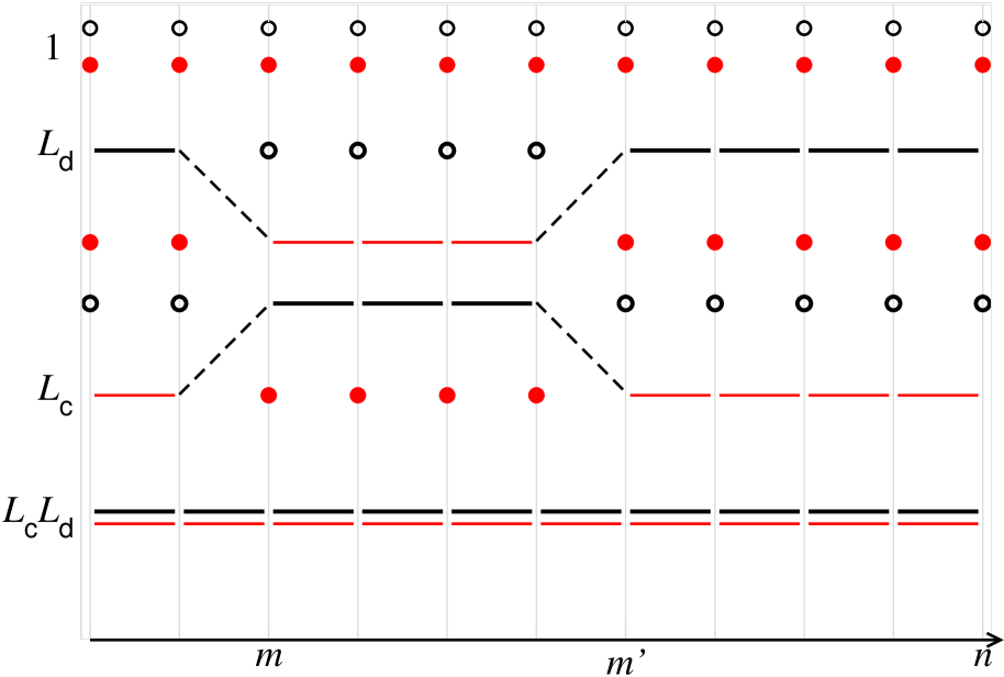
Figure 1: Typical world lines of a two-site system. Thick (thin) lines denote the elementary processes with the electron sitting on the impurity (“band”) site. Full (empty) circles denote the elementary processes with a hole sitting on the “band” (impurity) site. Dashed lines represent hopping processes. The horizontal axis runs with the time steps, while in the vertical direction different sites are displayed.

If we now return to our representation the contributions of the world lines to the partition function follow in a similar fashion, except for that i) the factor corresponding to hopping process at time step $m$ is given by $\delta Vx_{m}$, and ii) the particle line at time step $n$ corresponding to the electron sitting on the impurity site results in a factor $L_{n}$. Accordingly the contribution of the world line labeled by $L_{\rm c}$ in Fig. 1 to $\mbox{det}\left[S_{0}\right]$ is:

$$\left(\prod_{n=1}^{m-1}L_{\rm c}\right)\delta Vx_{m}\left(\prod_{n=m+1}^{m^{\prime}-1}L_{n}\right)\delta Vx_{m^{\prime}}\left(\prod_{n=m^{\prime}+1}^{N}L_{\rm c}\right),$$ (57)

while the world line labeled by $L_{\rm d}$ in Fig. 1 yields

$$\left(\prod_{n=1}^{m-1}L_{n}\right)\delta Vx_{m}\left(\prod_{n=m+1}^{m^{\prime}-1}L_{\rm c}\right)\delta Vx_{m^{\prime}}\left(\prod_{n=m^{\prime}+1}^{N}L_{n}\right).$$ (58)

3.1.2 Connecting with the hamiltonian language

We observe that the structure of Eq. (56) is not manifestly translationally invariant in time. For this reason, we proceed to bring Eq. (56) into a form where no particular time step is singled out. We note that the (row) column vector in Eq. (56) can be identified with the (rows) columns of the matrix blocks $\left[K^{(n)}\right]$ — disregarding the cancelling minus signs. Accordingly, we can rewrite Eq. (56) as:

$$\mbox{det}\left[S_{0}\right] =\sum_{\{\alpha_{2},\ldots,\alpha_{N}\}}~{}K^{(2),1}_{1\alpha_{2}}~{}K^{(3),1}_{\alpha_{2}\alpha_{3}}\ldots K^{(N),1}_{\alpha_{N-1}\alpha_{N}}K^{(1),1}_{\alpha_{N}1}$$ (59)

$$+\sum_{\{\alpha_{2},\ldots,\alpha_{N}\}}~{}K^{(2),2}_{1\alpha_{2}}~{}K^{(3),2}_{\alpha_{2}\alpha_{3}}\ldots K^{(N),2}_{\alpha_{N-1}\alpha_{N}}K^{(1),2}_{\alpha_{N}1}$$

$$+\sum_{\{\alpha_{2},\ldots,\alpha_{N}\}}~{}K^{(2),3}_{2\alpha_{2}}~{}K^{(3),3}_{\alpha_{2}\alpha_{3}}\ldots K^{(N),3}_{\alpha_{N-1}\alpha_{N}}K^{(1),3}_{\alpha_{N}2}$$

$$+\sum_{\{\alpha_{2},\ldots,\alpha_{N}\}}~{}K^{(2),4}_{1\alpha_{2}}~{}K^{(3),4}_{\alpha_{2}\alpha_{3}}\ldots K^{(N),4}_{\alpha_{N-1}\alpha_{N}}K^{(1),4}_{\alpha_{N}1},$$

since the matrices $\left[K^{(n)}\right]$ are block diagonal and symmetric. Observe that the first and last lower index in line three of Eq. (59) is not 1 but 2.

In Eq. (59), the first sum is equal to 1; the second and third sums are the diagonal elements of the matrix product $\prod_{n=1}^{N}\left(\begin{array}[]{cc}L_{\rm c}&\delta Vx_{n}\\ \delta Vx_{n}&L_{n}\end{array}\right)$, respectively. The last sum is equal to $L_{\rm c}^{N}\prod_{n=1}^{N}L_{n}$. Therefore Eq. (59) reduces to the trace of a 4$\times$4 matrix that is the product of the $N$ block diagonal matrices $\left[{\mathcal{K}}_{n}\right]$ whose elements are $\left[K^{(n),1}\right]$, $\left[K^{(n),2}\right]$ and $\left[K^{(n),4}\right]$, respectively:

$$\mbox{det}\left[S_{0}\right]=\mbox{Tr}\prod_{n=1}^{N}\left[{\mathcal{K}}_{n}\right],$$ (60)

where the matrix $\left[{\mathcal{K}}_{n}\right]$ is given by:

$$\left[{\mathcal{K}}_{n}\right]=\left(\begin{array}[]{cccc}1&{}\hfil&{}\hfil&{}\hfil\\ {}\hfil&L_{\rm c}&\delta Vx_{n}&{}\hfil\\ {}\hfil&\delta Vx_{n}&L_{n}&{}\hfil\\ {}\hfil&{}\hfil&{}\hfil&L_{\rm c}L_{n}\end{array}\right).$$ (61)

Here, it is of interest to note that we have established a direct link between the world line picture embodied in the 6$\times$6 matrices $\left[K^{(n)}\right]$ and the simpler description in terms of quantum states in the Fock space through the 4$\times$4 matrices $\left[{\mathcal{K}}_{n}\right]$. Indeed, when performing the world line expansion using Eq. (56), the propagation matrices $\left[K^{(n)}\right]$ acquire an involved structure following from the initial conditions attached to the world lines. This is best seen in the one-electron sub-space: at time-step one, the electron may either be on site c or on site d (see Fig. 1), and the corresponding dynamics is governed by the matrices $\left[K^{(n),2}\right]$ and $\left[K^{(n),3}\right]$. Summing up all these world lines yields the one-electron contribution to $\mbox{det}\left[S_{0}\right]$. Thus, one needs to handle two 2$\times$2 matrices, one in each case. In contrast, a single 2$\times$2 matrix needs to be treated on the level of Eq. (60).

In the above form of the fermionic determinant, Eq. (60), the time steps are decoupled, which greatly simplifies the projection onto the physical Hilbert space. Indeed, in terms of the matrix $\left[q\right]$ given by:

$$\left[q\right]\equiv{\mathcal{P}_{n}}\left(\left[{\mathcal{K}}_{n}\right]\right)=\left(\begin{array}[]{cccc}1&{}\hfil&{}\hfil&{}\hfil\\ {}\hfil&L_{\rm c}&\delta V&{}\hfil\\ {}\hfil&\delta V&L_{\rm d}&{}\hfil\\ {}\hfil&{}\hfil&{}\hfil&L_{\rm c}L_{\rm d}\end{array}\right),$$ (62)

we obtain the partition function ${\mathcal{Z}}_{0}$ as:

$${\mathcal{Z}}_{0}=\lim_{N\rightarrow\infty}\mbox{Tr}\prod_{n=1}^{N}\left[q\right]=\!\!\lim_{N\rightarrow\infty}\!\!\mbox{Tr}\left[1\mbox{I}_{4}\!\!-\!\delta\left(\begin{array}[]{cccc}0&{}\hfil&{}\hfil&{}\hfil\\ {}\hfil&\epsilon_{\rm c}-\mu&-V&{}\hfil\\ {}\hfil&-V&\epsilon_{\rm d}-\mu&{}\hfil\\ {}\hfil&{}\hfil&{}\hfil&\epsilon_{\rm c}+\epsilon_{\rm d}-2\mu\end{array}\right)\right]^{N}$$ (67)

Namely, we recover here the hamiltonian matrix in the Fock space. Therefore the expansion of $\mbox{det}\left[S_{0}\right]$ in minors together with the recurrence relations, Eq. (50), allows for a correspondence between the ensemble of the world lines and the hamiltonian matrix. It is apparent that the complexity of this interrelation depends on whether or not the system is in an eigenstate at time step one. If this is the case, there is one single straight world line, and the connection is obvious. Otherwise there is a proliferation of world lines, here controlled by the matrices $\left[K^{(n),2}\right]$ and $\left[K^{(n),3}\right]$, which recombine to yield the contribution resulting from the 2$\times$2 block of the matrix $\left[{\mathcal{K}}_{n}\right]$. A result equivalent to Eq. (67) was already obtained by Barnes BAR77 , though in a totally different fashion.

3.2 Hole density

In our path integral formalism, the expectation value of the amplitude of the slave boson field at time step $m$ is $\langle x_{m}\rangle$. It simply represents the hole density $1-n_{\rm d}$ which can be written as $\langle x_{m}\rangle=\langle b^{\dagger}_{m}b^{\phantom{\dagger}}_{m-1}\rangle$ where $b$ represents the original Barnes slave boson, and $\langle x_{m}\rangle$ is finite. In contrast the expectation values of the boson operators are zero: $\langle b^{\dagger}_{m}\rangle=\langle b_{m}\rangle=0$, for each time step because of the fluctuations of their respective phase factor, in agreement with Elitzur’s theorem. Note that expectation values of higher order moments of $x_{m}$ are also non zero: $\langle x^{a}_{m}\rangle=\langle x_{m}\rangle\neq 0$ for any real positive parameter $a$.

In the case of spinless fermions we calculate $\langle x_{m}\rangle$ as:

$${\mathcal{Z}}_{0}\langle x_{m}\rangle = \lim_{\begin{subarray}{c}N\rightarrow\infty\\ W\rightarrow\infty\end{subarray}}{\mathcal{P}_{1}}\ldots{\mathcal{P}_{N}}~{}\left(\mbox{det}\left[S_{0}\right]~{}x_{m}\right)$$

$$= \lim_{\begin{subarray}{c}N\rightarrow\infty\\ W\rightarrow\infty\end{subarray}}{\mathcal{P}_{1}}\ldots{\mathcal{P}_{N}}~{}\left(x_{m}\mbox{Tr}~{}\prod_{n=1}^{N}\left[{\mathcal{K}}_{n}\right]\right).$$

If we introduce the 4$\times$4 matrix $\left[{\mathcal{Q}}_{X}\right]\equiv{\mathcal{P}}_{n}(x_{n}\left[{\mathcal{K}}_{n}\right])$ for all $n$, and $\left[{\mathcal{Q}}\right]$ the 4$\times$4 diagonal matrix that satisfies $\left[q\right]=\left[U_{\mathcal{Q}}\right]\left[{\mathcal{Q}}\right]\left[{U}_{\mathcal{Q}}\right]^{\dagger}$, $\left[U_{\mathcal{Q}}\right]$ being the eigenvector matrix, Eq. (3.2) becomes:

$${\mathcal{Z}}_{0}\langle x_{m}\rangle=\lim_{N\rightarrow\infty}\mbox{Tr}\left(\left[{\mathcal{Q}}\right]^{N-1}\left[{U}_{\mathcal{Q}}\right]^{\dagger}\left[{\mathcal{Q}}_{X}\right]\left[U_{\mathcal{Q}}\right]\right).$$ (69)

Using Eqs. (8)–(10), and the $\delta\rightarrow 0$ limit, we obtain that the matrix $\left[{\mathcal{Q}}_{X}\right]$ reduces to the representation of the hole density operator on the impurity in the Fock space:

$$\left[{\mathcal{Q}}_{X}\right]_{i,j}=\delta_{i,1}~{}\delta_{j,1}+\delta_{i,2}~{}\delta_{j,2}.$$ (70)

Correspondingly, Eq. (69) expresses $\langle x_{m}\rangle$ as the averaged value of the hole density operator on the impurity, represented by its matrix elements in the basis of the eigenstates of the Hamiltonian ($\left[{U}_{\mathcal{Q}}\right]^{\dagger}\left[{\mathcal{Q}}_{X}\right]\left[U_{\mathcal{Q}}\right]$) and weighted by the Boltzmann factors $\frac{1}{{\mathcal{Z}}_{0}}\left[{\mathcal{Q}}\right]^{N-1}$. Therefore, in contrast to a Bose condensate, $\langle x_{m}\rangle$ is generically finite and may only vanish for zero hole concentration. Its numerical evaluation will be presented in a forthcoming paper OUE07 .

3.3 Density-density correlation function

To obtain further insight into the approach, it is of interest to compute dynamical correlation functions. Probably, the simplest one is provided by the hole density autocorrelation function on the impurity site. When expressed in terms of eigenstates of the Hamiltonian, it takes the form:

$$\langle\left(1-n_{\rm d}(m\delta)\right)\left(1-n_{\rm d}(\delta)\right)\rangle=\frac{\displaystyle 1}{\displaystyle{\mathcal{Z}}_{0}}~{}\sum_{\alpha,\alpha^{\prime}}e^{\delta(m-N)E_{\alpha}}e^{-m\delta E_{\alpha^{\prime}}}|\langle\psi_{\alpha}|1-n_{\rm d}|\psi_{\alpha^{\prime}}\rangle|^{2},$$ (71)

where the eigenvalues $E_{\alpha}$ can be obtained from the diagonalization of the Hamiltonian. The latter can be read from, e. g., Eq. (67).

In our path integral representation, the autocorrelation function $\langle x_{1}x_{m}\rangle$ may be written as:

$${\mathcal{Z}}_{0}\langle x_{1}x_{m}\rangle = \lim_{\begin{subarray}{c}N\rightarrow\infty\\ W\rightarrow\infty\end{subarray}}{\mathcal{P}_{1}}\ldots{\mathcal{P}_{N}}~{}\left(\mbox{det}\left[S_{0}\right]~{}x_{1}x_{m}\right)$$

$$= \lim_{\begin{subarray}{c}N\rightarrow\infty\\ W\rightarrow\infty\end{subarray}}{\mathcal{P}_{1}}\ldots{\mathcal{P}_{N}}~{}\left(x_{1}x_{m}\mbox{Tr}~{}\prod_{n=1}^{N}\left[{\mathcal{K}}_{n}\right]\right),$$

which reduces to

$${\mathcal{Z}}_{0}\langle x_{1}x_{m}\rangle=\lim_{N\rightarrow\infty}\mbox{Tr}\left(\left[{\mathcal{Q}}_{X}\right]\left[q\right]^{m-2}\left[{\mathcal{Q}}_{X}\right]\left[q\right]^{N-m}\right),$$ (73)

after application of the projectors, Eqs. (8)–(13). If we now introduce the eigenvalues and eigenvectors of the Hamiltonian, Eq. (73) can be recast into:

$${\mathcal{Z}}_{0}\langle x_{1}x_{m}\rangle=\lim_{N\rightarrow\infty}\mbox{Tr}\left(\left[{\mathcal{Q}}\right]^{N-m}\left[{U}_{\mathcal{Q}}\right]^{\dagger}\left[{\mathcal{Q}}_{X}\right]\left[U_{\mathcal{Q}}\right]\left[{\mathcal{Q}}\right]^{m-2}\left[{U}_{\mathcal{Q}}\right]^{\dagger}\left[{\mathcal{Q}}_{X}\right]\left[U_{\mathcal{Q}}\right]\right).$$ (74)

In this form we recognize the standard expression in Eq. (71). Indeed, the combination $\left[{U}_{\mathcal{Q}}\right]^{\dagger}\left[{\mathcal{Q}}_{X}\right]\left[U_{\mathcal{Q}}\right]$ represents the matrix elements of the hole density operator in the basis of the eigenstates of the Hamiltonian, and the factors $\left[{\mathcal{Q}}\right]$ the exponential factors in Eq. (71).

4 Spin 1/2 system

We turn now to the spinful case. In this section, we show how results obtained for the spinless system are relevant and useful to derive in a straightforward fashion the corresponding quantities of the spin 1/2 system.

4.1 Partition function

Since up- and down-spins are decoupled, and since the fermionic contribution to the action is identical for both of them, we can write the fermionic determinant as: det$\left[S\right]$ = det$\left[S_{0}\right]^{2}$. This allows to express the determinant as the product of the traces of the matrix products $\prod_{n=1}^{N}\left[{\mathcal{K}}_{n}\right]$. By making use of the mixed product property of the Kronecker product: $\left(\left[A\right]\left[C\right]\right)\otimes\left(\left[B\right]\left[D\right]\right)=\left(\left[A\right]\otimes\left[B\right]\right)\left(\left[C\right]\otimes\left[D\right]\right)$, we obtain:

$$\mbox{det}\left[S\right]=\mbox{Tr}\prod_{n=1}^{N}\left[{\mathcal{K}}_{n}\right]\otimes\left[{\mathcal{K}}_{n}\right].$$ (75)

The partition function is obtained by combining Eqs. (75) and (6). Since the time steps are decoupled, the evaluation of the integrals over the $x$ and $\lambda$ fields is straightforward. The tensorial products $\left[{\mathcal{K}}_{n}\right]\otimes\left[{\mathcal{K}}_{n}\right]$ yield 16$\times$16 matrices, which, after application of the projectors ${\mathcal{P}}_{1}\ldots{\mathcal{P}}_{N}$, become block diagonal with a $4\times 4$ zero block. They all reduce to the same 12$\times$12 real symmetric matrix $\left[k\right]$. The matrix $\left[k\right]$ represents the projection of the tensor product $\left[{\mathcal{K}}_{n}\right]\otimes\left[{\mathcal{K}}_{n}\right]$ for all $n$ as

$$\left[k\right]_{i,j}={\mathcal{P}}_{n}(\left[{\mathcal{K}}_{n}\right]_{i_{1},j_{1}}\left[{\mathcal{K}}_{n}\right]_{i2,j2})$$ (76)

with the convention

$$i=\begin{cases}4(i_{1}-1)+i_{2}&\text{if ($1\leq i_{1}\leq 2$ and $1\leq i_{2}\leq 4$)}\\ &\quad\text{ and ($i_{1}=3$ and $1\leq i_{2}\leq 2$)},\\ i=i_{2}+10&\text{if ($i_{1}=4$ and $1\leq i_{2}\leq 2$).}\end{cases}$$ (77)

and similarly for $j$. The remaining matrix elements of the $16\times 16$ matrix form a vanishing $4\times 4$ separate block and have been discarded in Eq. (76). Finally we obtain a simple expression for the partition function ${\mathcal{Z}}$ of the two-site single impurity Anderson model:

$${\mathcal{Z}}=\lim_{N\rightarrow\infty}\mbox{Tr}~{}\left[k\right]^{N}.$$ (78)

with

$$\left[k\right]=\left(\begin{array}[]{cccccccccccc}1&&&&&&&&&&&\\ &L_{\rm c}&\delta V&&&&&&&&&\\ &\delta V&L_{\rm d}&&&&&&&&&\\ &&&L_{\rm c}L_{\rm d}&&&&&&&&\\ &&&&L_{\rm c}&0&0&0&\delta V&0&0&0\\ &&&&0&L_{\rm c}^{2}&L_{\rm c}\delta V&0&0&L_{\rm c}\delta V&0&0\\ &&&&0&L_{\rm c}\delta V&L_{\rm c}L_{\rm d}&0&0&0&0&0\\ &&&&0&0&0&L_{\rm c}^{2}L_{\rm d}&0&0&0&0\\ &&&&\delta V&0&0&0&L_{\rm d}&0&0&0\\ &&&&0&L_{\rm c}\delta V&0&0&0&L_{\rm c}L_{\rm d}&0&0\\ &&&&0&0&0&0&0&0&L_{\rm c}L_{\rm d}&0\\ &&&&0&0&0&0&0&0&0&L_{\rm c}^{2}L_{\rm d}\end{array}\right).$$ (79)

When expanded to lowest order in $\delta$, the blocks of $\left[k\right]$ represent the hamiltonian matrix in the Fock space, in the same fashion as in Eq. (67). Diagonalizing these blocks yields the expected expression of the partition function ${\mathcal{Z}}$:

$${\mathcal{Z}} = 1+3\exp\left[-\beta\left(\epsilon_{\rm c}+\epsilon_{\rm d}-2\mu\right)\right]+2\exp\left[-\beta\left(2\epsilon_{\rm c}+\epsilon_{\rm d}-3\mu\right)\right]$$ (80)

$${}+2\sum_{j=\pm 1}\exp\left[-\beta\left(\frac{\displaystyle\epsilon_{\rm c}+\epsilon_{\rm d}}{\displaystyle 2}-\mu+j\sqrt{\left(\frac{\displaystyle\epsilon_{\rm c}-\epsilon_{\rm d}}{\displaystyle 2}\right)^{2}+V^{2}}\right)\right]$$

$${}+\sum_{j=\pm 1}\exp\left[-\beta\left(\frac{\displaystyle 3\epsilon_{\rm c}+\epsilon_{\rm d}}{\displaystyle 2}-2\mu+j\sqrt{\left(\frac{\displaystyle\epsilon_{\rm c}-\epsilon_{\rm d}}{\displaystyle 2}\right)^{2}+2V^{2}}\right)\right].$$

Through the exact calculation of the functional integrals we have recovered this result that can also be derived from the diagonalization of the Hamiltonian. Note that $V$ is multiplied by different coefficients in the one-particle and two-particle states. In contrast to the spinless case Eq. (67) the eigenvalues of the hamiltonian matrix entering Eq. (79) result from entangled states, the entanglement being achieved by the projection onto the physical Fock space in Eq. (76). Note that we here obtained the hamiltonian matrix without having explicitely used any basis of the Fock space. It naturally arose as the projected tensor product of the basis appropriate to the spinless case.

4.2 Hole density and autocorrelation function

In the spinful case, the hole density $\langle x_{m}\rangle$ is given by:

$${\mathcal{Z}}\langle x_{m}\rangle = \lim_{\begin{subarray}{c}N\rightarrow\infty\\ W\rightarrow\infty\end{subarray}}{\mathcal{P}_{1}}\ldots{\mathcal{P}_{N}}~{}\left(\mbox{det}\left[S\right]~{}x_{m}\right)$$

$$= \lim_{\begin{subarray}{c}N\rightarrow\infty\\ W\rightarrow\infty\end{subarray}}{\mathcal{P}_{1}}\ldots{\mathcal{P}_{N}}~{}\left(x_{m}\mbox{Tr}~{}\prod_{n=1}^{N}\left[{\mathcal{K}}_{n}\right]\otimes\left[{\mathcal{K}}_{n}\right]\right)$$

For the spin 1/2 case, the counterpart of the matrix $\left[{\mathcal{Q}}_{X}\right]$ is the matrix $\left[{\mathcal{K}}_{X}\right]\equiv{\mathcal{P}}_{n}(x_{n}\left[{\mathcal{K}}_{n}\right]\otimes\left[{\mathcal{K}}_{n}\right])$. It is a 12$\times$12 matrix, the elements of which may be expressed as:

$$\left[{\mathcal{K}}_{X}\right]_{i,j}=\delta_{i,1}~{}\delta_{j,1}+\delta_{i,2}~{}\delta_{j,2}+\delta_{i,5}~{}\delta_{j,5}+\delta_{i,6}~{}\delta_{j,6},$$ (82)

using Eqs. (8)–(13), in the $\delta\rightarrow 0$ limit. In this form it represents the hole density operator on the impurity site in the Fock space. Thus Eq. (4.2) becomes

$${\mathcal{Z}}\langle x_{m}\rangle=\lim_{N\rightarrow\infty}\mbox{Tr}\left(\left[{\mathcal{K}}_{X}\right]\left[k\right]^{N-1}\right),$$ (83)

which has exactly the same form as for the spinless case and a similar interpretation applies.

As for autocorrelation functions such as $\langle x_{1}x_{m}\rangle$, we can adopt the same procedure to obtain

$${\mathcal{Z}}\langle x_{1}x_{m}\rangle=\lim_{N\rightarrow\infty}\mbox{Tr}\left(\left[{\mathcal{K}}_{X}\right]\left[k\right]^{m-2}\left[{\mathcal{K}}_{X}\right]\left[k\right]^{N-m}\right),$$ (84)

which, when again introducing the eigenstates of the Hamiltonian, can also be identified to the ordinary expression in Eq. (71). On the formal level, the use of the slave boson representation in the radial gauge greatly simplifies the evaluation of the dynamical correlation functions of the operators that can be represented by the radial slave bosons.

5 Green’s function

We turn to the impurity Green’s function $G_{\sigma}(q-p)$. When expressed in terms of the eigenvalues of the Hamiltonian, $E_{\alpha}$ — which can be read from, e. g., Eq. (80) for spin 1/2 — it reads:

$${\mathcal{Z}}G_{\sigma}(q-p)=-\sum_{\alpha,\alpha^{\prime}}e^{\delta(q-N-p)E_{\alpha}}\langle\psi_{\alpha}|d_{\sigma}|\psi_{\alpha^{\prime}}\rangle e^{\delta(p-q)E_{\alpha^{\prime}}}\langle\psi_{\alpha^{\prime}}|d^{\dagger}_{\sigma}|\psi_{\alpha}\rangle,$$ (85)

In the radial gauge the creation and annihilation operators are expressed in terms of auxiliary fields as given in Eqs. (2) and (3). We obtain $G_{\sigma}(q-p)$ as follows:

$${\mathcal{Z}}G_{\sigma}(q-p)=-\lim_{\begin{subarray}{c}N\rightarrow\infty\\ W\rightarrow\infty\end{subarray}}\prod_{n=1}^{N}\int \prod_{\sigma^{\prime}=\downarrow,\uparrow}D[f_{n,\sigma^{\prime}},f^{\dagger}_{n,\sigma^{\prime}}]D[c_{n,\sigma^{\prime}},c^{\dagger}_{n,\sigma^{\prime}}]$$

$$\times \int_{-\infty}^{\infty}\frac{\displaystyle\delta{\rm d}\lambda_{n}}{\displaystyle 2\pi}\int_{-\infty}^{\infty}{\rm d}x_{n}~{}e^{-S}f^{\phantom{\dagger}}_{q,\sigma}f^{\dagger}_{p,\sigma}x_{q+1}x_{p},$$

in the language of functional integrals. Note that the three other Green’s functions involving the three expectation values: $\langle d^{\phantom{\dagger}}_{q,\sigma}c^{\dagger}_{p,\sigma}\rangle$, $\langle c^{\phantom{\dagger}}_{q,\sigma}d^{\dagger}_{p,\sigma}\rangle$ and $\langle c^{\phantom{\dagger}}_{q,\sigma}c^{\dagger}_{p,\sigma}\rangle$, can be calculated in the same fashion, except that they are simpler to evaluate since they contain at most one amplitude of the slave bosonic field, $x$, unlike the one we chose to study.

5.1 Derivation of the pseudofermion Green’s function

Following standard procedures (see, e. g., Negele and Orland NEG88 ), we cast Eq. (5) into the form:

$${\mathcal{Z}}G_{\sigma}(q-p)=-\lim_{\begin{subarray}{c}N\rightarrow\infty\\ W\rightarrow\infty\end{subarray}}{\mathcal{P}_{1}}\ldots{\mathcal{P}_{N}}~{}\left(\mbox{det}\left[S_{0}\right]{\mathcal{G}}_{p,q}~{}x_{p}x_{q+1}\right),$$ (87)

where ${\mathcal{G}}_{p,q}$ is the minor of one of the matrix elements of the 2$\times$2 block that shares the same row labels as $\left[{\mathcal{L}}_{p}\right]$ and column labels as $\left[{\mathcal{L}}_{q+1}\right]$ in the matrix $\left[S_{0}\right]$ as defined in Eq. (18) (if $q=N$ then the block to be considered is $\left[{\mathcal{L}}_{1}\right]$). The minor ${\mathcal{G}}_{p,q}$ is the unprojected pseudofermion Green’s function.

For the subsequent calculations we set $p=N-m+1$ and $q=N$. The minor ${\mathcal{G}}_{N-m+1,N}$ can be calculated as:

$${\mathcal{G}}_{N-m+1,N}=\frac{\displaystyle\partial}{\displaystyle\partial a}~{}\mbox{det}\left[S(a;m)\right],$$ (88)

where $\left[S(a;m)\right]$ is given by:

$$\left[S(a;m)\right]_{i,j}=\left[S_{0}\right]_{i,j}+a\delta_{i,2(N-m+1)}\delta_{j,2N}.$$ (89)

To calculate $\mbox{det}\left[S(a;m)\right]$, we find it convenient to move the last two columns to the left in the matrix $\left[S(a;m)\right]$ in Eq. (89). In the same fashion as for $\mbox{det}\left[S_{0}\right]$, we expand $\mbox{det}\left[S(a;m)\right]$ along the first two columns. Once the derivative of $\mbox{det}\left[S(a;m)\right]$ with respect to $a$ is calculated we obtain the three contributions:

$$\frac{\displaystyle\partial}{\displaystyle\partial a}~{}\mbox{det}\left[S(a;m)\right]=-1\times{\mathcal{M}}_{1,a}^{\overline{1}}+L_{\rm c}{\mathcal{M}}_{L_{\rm c},a}^{\overline{1}}+\delta Vx_{1}{\mathcal{M}}_{\delta,a}^{\overline{1}},$$ (90)

where the three minors ${\mathcal{M}}_{1,a}^{\overline{1}}$, ${\mathcal{M}}_{L_{\rm c},a}^{\overline{1}}$ and ${\mathcal{M}}_{\delta,a}^{\overline{1}}$ are defined in the appendix. They can be expressed as linear combinations of ${\mathcal{M}}_{1,a}^{\overline{2}}$, $M_{L_{\rm c},a}^{\overline{2}}$ and ${\mathcal{M}}_{\delta,a}^{\overline{2}}$ in the same fashion as for the minors defined in the previous sections. They also follow a recurrence relation that reads:

$$\left(\begin{array}[]{c}{\mathcal{M}}^{\overline{n}}_{1,a}\\ {\mathcal{M}}^{\overline{n}}_{L_{\rm c},a}\\ {\mathcal{M}}^{\overline{n}}_{\delta,a}\end{array}\right)=\left(\begin{array}[]{ccc}1&0&0\\ 0&L_{\rm c}&\delta Vx_{n+1}\\ 0&\delta Vx_{n+1}&L_{n+1}\end{array}\right)\left(\begin{array}[]{c}{\mathcal{M}}^{\overline{n+1}}_{1,a}\\ {\mathcal{M}}^{\overline{n+1}}_{L_{\rm c},a}\\ {\mathcal{M}}^{\overline{n+1}}_{\delta,a}\end{array}\right),$$ (100)

up to time step $n=N-m$. Here we recognize the blocks defined in Eqs. (51) and (54) entering the matrix $[K^{(n+1)}]$ which we encountered during the evaluation of the partition function. Then, ${\mathcal{M}}_{1,a}^{\overline{N-m}}$, ${\mathcal{M}}_{L_{\rm c},a}^{\overline{N-m}}$ and ${\mathcal{M}}_{\delta,a}^{\overline{N-m}}$ are linear combinations of the minors ${\mathcal{M}}_{1,4}^{\overline{N-m+1}}$ and ${\mathcal{M}}_{3,4}^{\overline{N-m+1}}$:

$$\left(\begin{array}[]{c}{\mathcal{M}}^{\overline{N-m}}_{1,a}\\ {\mathcal{M}}^{\overline{N-m}}_{L_{\rm c},a}\\ {\mathcal{M}}^{\overline{N-m}}_{\delta,a}\end{array}\right)=\left(\begin{array}[]{cc}-1&0\\ 0&L_{\rm c}\\ 0&\delta Vx_{N-m+1}\end{array}\right)\left(\begin{array}[]{c}{\mathcal{M}}^{\overline{N-m+1}}_{1,4}\\ {\mathcal{M}}^{\overline{N-m+1}}_{3,4}\end{array}\right).$$ (109)

The minors ${\mathcal{M}}_{1,4}^{\overline{n}}$ and ${\mathcal{M}}_{3,4}^{\overline{n}}$ are tightly related to $M_{1,4}^{\overline{n}}$ and $M_{3,4}^{\overline{n}}$: they are also built on a matrix similar to $\left[S_{0}\right]$, but with the difference that only the time steps $m$ with $m>n$ are included. ${\mathcal{M}}_{i,j}^{\overline{n}}$ is a minor of this matrix, where the first two columns and both the $i$-th and $j$-th rows are removed. Accordingly, the recurrence relations for ${\mathcal{M}}_{1,4}^{\overline{N-m+1}}$ and ${\mathcal{M}}_{3,4}^{\overline{N-m+1}}$ are also given in Eq. (50) and hence we also need to introduce the minor ${\mathcal{M}}_{1,3}^{\overline{N-m+1}}$. Thus, their evaluation involves the blocks of Eqs. (54) and (55), which enter the matrix $[K^{(n+1)}]$ jointly with the last three components of the column vector in Eq. (56), taken at time step $N$. Therefore, to calculate ${\mathcal{G}}_{N-m+1,N}$ as defined above we have to consider the following set of six minors: ${\mathcal{M}}_{1,a}$, ${\mathcal{M}}_{L_{\rm c},a}$, ${\mathcal{M}}_{\delta,a}$ for time steps $1\leq n\leq N-m$, and ${\mathcal{M}}_{1,3}$, ${\mathcal{M}}_{1,4}$ and ${\mathcal{M}}_{3,4}$ for time steps $N-m+2\leq n\leq N$.

Combining the above steps, we can write the unprojected pseudofermion Green’s function as:

$${\mathcal{G}}_{N-m+1,N}= \mbox{Tr}\left[\left[K^{(N)}_{f}\right]\times\left(\prod_{n=N-1}^{N-m+2}\left[K^{(n)}_{>}\right]\right)\right.$$

$$~{}~{}~{}~{}\times\left.\left[K^{(N-m+1)}_{f^{\dagger}}\right]\times\left(\prod_{n=N-m}^{1}\left[K^{(n)}_{<}\right]\right)\right],$$

where the time steps enter in decreasing order. The 6$\times$6 matrices $\left[K^{(N)}_{f}\right]$ $\left(\left[K^{(N-m+1)}_{f^{\dagger}}\right]\right)$ representing the annihilation (creation) of a fermion in the world line language are given by

$$\left[K^{(N)}_{f}\right]_{i,j} = \delta Vx_{N}~{}\delta_{i,1}~{}\delta_{j,4}+L_{N}~{}\delta_{i,2}~{}\delta_{j,5}+L_{\rm c}L_{N}~{}\delta_{i,2}~{}\delta_{j,6}$$

$$\left[K^{(N-m+1)}_{f^{\dagger}}\right]_{i,j} = 1~{}\delta_{i,5}~{}\delta_{j,1}+L_{\rm c}~{}\delta_{i,6}~{}\delta_{j,2}+\delta Vx_{N-m+1}~{}\delta_{i,6}~{}\delta_{j,3}~{}.$$ (111)

In Eq. (5.1), $\left[K^{(n)}_{<}\right]$ is a 6 $\times$ 6 block diagonal matrix the non zero elements of which are the two blocks $\left[K^{(n),1}\right]$ and $\left[K^{(n),2}\right]$ defined in Eqs. (51) and (54). The matrix $\left[K^{(n)}_{>}\right]$ is also 6 $\times$ 6 block diagonal matrix determined by

$$\left[K^{(n)}_{>}\right]=\left[K^{(n)}\right]-\left[K^{(n)}_{<}\right].$$ (112)

Equation (5.1) can also be interpreted on the basis of Fig. 1. In fact, computing $\langle d^{\phantom{\dagger}}_{N,\sigma}d^{\dagger}_{N-m+1,\sigma}\rangle$ can be visualized as the resummation of particular subsets of world lines. They are naturally split into sets involving $L_{\rm d}$ for $N-m+2<n<N-1$, in which case $\left[K^{(n)}_{>}\right]$ is controlling the dynamics of the world lines; and sets excluding $L_{\rm d}$ for $1<n<N-m$, in which case $\left[K^{(n)}_{<}\right]$ controls the dynamics. The transition from the first (second) subset to the second (first) is taken care of by the matrix $\left[K^{(N-m+1)}_{f^{\dagger}}\right]$ $\left(\left[K^{(N)}_{f}\right]\right)$.

This expression for the Green’s function in the world line language can also be related to its counterpart in the hamiltonian language. Indeed, the trace of the matrix product in Eq. (5.1) can be written in terms of 4$\times$4 matrices:

$${\mathcal{G}}_{N-m+1,N}=\mbox{Tr}\left(\left[F_{N}\right]\times\left(\prod_{n=N-1}^{N-m+2}\left[{\mathcal{K}}^{>}_{n}\right]\right)\times\left[\Phi_{N-m+1}\right]\times\left(\prod_{n=N-m}^{1}\left[{\mathcal{K}}^{<}_{n}\right]\right)\right),$$ (113)

where

$$\left[\Phi_{N-m+1}\right]=\left(\begin{array}[]{cccc}0&0&0&0\\ 0&0&0&0\\ 1&0&0&0\\ 0&L_{\rm c}&\delta Vx_{N-m+1}&0\end{array}\right)~{}~{}~{}~{}\mbox{and}~{}~{}~{}~{}\left[F_{N}\right]=\left(\begin{array}[]{cccc}0&\delta Vx_{N}&L_{N}&0\\ 0&0&0&L_{\rm c}L_{N}\\ 0&0&0&0\\ 0&0&0&0\end{array}\right),$$ (114)

characterize the creation and annihilation of an electron, respectively. The matrices $\left[{\mathcal{K}}^{<}_{n}\right]$ and $\left[{\mathcal{K}}^{>}_{n}\right]$ result from $\left[{\mathcal{K}}_{n}\right]$ as:

$$\left[{\mathcal{K}}^{<}_{n}\right]_{i,j} = \left[{\mathcal{K}}^{n}\right]_{i,j}-L_{\rm c}L_{n}~{}\delta_{i,4}~{}\delta_{j,4}\;,$$

$$\left[{\mathcal{K}}^{>}_{n}\right]_{i,j} = \left[{\mathcal{K}}^{n}\right]_{i,j}-\delta_{i,1}~{}\delta_{j,1}~{}.$$ (115)

5.2 Spinless case

Now that the unprojected pseudofermion Green’s function has been converted to a compact form, we can evaluate the physical Green’s function which, in the spinless case, reads:

$${\mathcal{Z}}_{0}G_{0}(q-p) = -\lim_{\begin{subarray}{c}N\rightarrow\infty\\ W\rightarrow\infty\end{subarray}}{\mathcal{P}_{1}}\ldots{\mathcal{P}_{N}}~{}\mbox{Tr}\left[x_{1}x_{N-m+1}\left[F_{N}\right]\times\left(\prod_{n=N-1}^{N-m+2}\left[{\mathcal{K}}^{>}_{n}\right]\right)\right.$$ (116)

$$\times \left.\left[\Phi_{N-m+1}\right]\times\left(\prod_{n=N-m}^{1}\left[{\mathcal{K}}^{<}_{n}\right]\right)\right].$$

With the application of the projectors ${\mathcal{P}_{1}}\ldots{\mathcal{P}_{N}}$, we obtain:

$${\mathcal{Z}}_{0}G_{0}(q-p)=-\lim_{N\rightarrow\infty}\mbox{Tr}\left(\left[{\mathcal{Q}}_{X}\right]\left[{\mathcal{F}}\right]\left[q^{>}\right]^{m-2}\left[\phi\right]\left[q^{<}\right]^{N-m-1}\right),$$ (117)

where $\left[{\mathcal{Q}}_{X}\right]$ is given by Eq. (70). The matrices $\left[\phi\right]$ and $\left[{\mathcal{F}}\right]$ are defined as $\left[\phi\right]\equiv{\mathcal{P}}_{N-m+1}\left(x_{N-m+1}\left[\Phi_{N-m+1}\right]\right)$ and $\left[{\mathcal{F}}\right]\equiv{\mathcal{P}}_{N}\left(\left[F_{N}\right]\right)$ respectively. They can be read off from Eq. (114) if $x$ is replaced by 1, and $L_{n}$ by $L_{\rm d}$. Note that $\left[\phi\right]=\left[{\mathcal{F}}\right]^{\dagger}$ only in the limit $\delta\rightarrow 0$ when $L_{\rm c}\rightarrow 1$ and $L_{\rm d}\rightarrow 1$. In the limit $\delta\rightarrow 0$, they coincide with the matrix representations of the operators $f^{\dagger}$ and $f$ respectively. The matrices $\left[q^{<}\right]$ and $\left[q^{>}\right]$ are given by $\left[q^{<}\right]\equiv{\mathcal{P}}_{n}(\left[{\mathcal{K}}^{<}_{n}\right])$ and $\left[q^{>}\right]\equiv{\mathcal{P}}_{n}(\left[{\mathcal{K}}^{>}_{n}\right])$ respectively, and are easily related to $\left[q\right]$:

$$\left[q^{<}\right]_{i,j} = \left[q\right]_{i,j}-L_{\rm c}L_{\rm d}~{}\delta_{i,4}~{}\delta_{j,4}$$

$$\left[q^{>}\right]_{i,j} = \left[q\right]_{i,j}-~{}\delta_{i,1}~{}\delta_{j,1}.$$ (118)

we can now reshape Eq. (117) into the form:

$${\mathcal{Z}}_{0}G_{0}(q-p) = -\lim_{N\rightarrow\infty}\mbox{Tr}\left[\left[{\mathcal{Q}}^{<}\right]^{N-m-1}\left(\left[U_{\mathcal{Q}}\right]^{\dagger}\left[{\mathcal{Q}}_{X}\right]\left[{\mathcal{F}}\right]\left[U_{\mathcal{Q}}\right]\right)\right.$$

$$~{}~{}~{}~{}~{}~{}~{}~{}~{}~{}~{}~{}~{}~{}\times\left.\left[{\mathcal{Q}}^{>}\right]^{m-2}\left(\left[U_{\mathcal{Q}}\right]^{\dagger}\left[\phi\right]\left[U_{\mathcal{Q}}\right]\right)\right],$$

where $\left[{\mathcal{Q}}^{<}\right]$ and $\left[{\mathcal{Q}}^{>}\right]$ are obtained from the diagonalization of $\left[q^{<}\right]$ and $\left[q^{>}\right]$, respectively. Note that the same matrix $\left[U_{\mathcal{Q}}\right]$ diagonalizes the matrices $\left[q\right],~{}\left[q^{<}\right]$, and $\left[q^{>}\right]$.

In Eq. (5.2), the product $\left[U_{\mathcal{Q}}\right]^{\dagger}\left[{\mathcal{Q}}_{X}\right]\left[{\mathcal{F}}\right]\left[U_{\mathcal{Q}}\right]$ is the representation of the annihilation operator $d$ in the basis of the eigenstates of the Hamiltonian, while $\left[U_{\mathcal{Q}}\right]^{\dagger}\left[\phi\right]\left[U_{\mathcal{Q}}\right]$ represents $d^{\dagger}$, as can be easily verified explicitly in the limit $\delta\rightarrow 0$. The factors $\left[{\mathcal{Q}}^{>}\right]$ and $\left[{\mathcal{Q}}^{<}\right]$ determine the time evolution. Therefore Eq. (5.2) can be easily identified with Eq. (85). Note that all eigenvalues seem to contribute to the Green’s function in Eq. (85), and only the matrix elements of the creation (annihilation) operators restrict the set of eigenvalues that effectively contribute to the Green’s function. In contrast, in Eq. (5.2) some of these restrictions are contained in the factors $\left[{\mathcal{Q}}^{>}\right]$ and $\left[{\mathcal{Q}}^{<}\right]$ which replace the full set of eigenvalues, that would be contained in the matrix $\left[{\mathcal{Q}}\right]$.

It is tempting to compare the physical electron Green’s function (including the factors $x$) to the projected pseudo-fermion Green’s function (without the factors $x$). Straightforward algebra yields:

$$\lim_{\delta\rightarrow 0}~{}{\mathcal{P}}_{N-m+1}\left(x_{N-m+1}\left[\Phi_{N-m+1}\right]\right)=\lim_{\delta\rightarrow 0}~{}{\mathcal{P}}_{N-m+1}\left(\left[\Phi_{N-m+1}\right]\right),$$ (120)

and

$$\lim_{\delta\rightarrow 0}~{}{\mathcal{P}}_{1}{\mathcal{P}}_{N}\left(x_{1}\left[K_{1}^{<}\right]\left[F_{N}\right]\right)=\lim_{\delta\rightarrow 0}~{}{\mathcal{P}}_{1}{\mathcal{P}}_{N}\left(\left[K_{1}^{<}\right]\left[F_{N}\right]\right).$$ (121)

Therefore, as a particularity of the spinless case, the factors $x$ in Eq. (116) play no role, and both Green’s functions coincide. Consequently the same result for the physical electron Green’s function would have been obtained by substituting $x$ by 1 in Eqs. (2) and (3), and accordingly in the fermionic contribution to the action $S_{f}$. Incidentally, such a procedure is in complete agreement with the original suggestion by Kotliar and Ruckenstein KOT86 to modify the expression of the physical electron operator by introducing square root factors, when extended to the spinless case.

5.3 Spin 1/2 system

Again, as shown below, results obtained for the spinless system can be immediately applied to derive the Green’s function in the spinful case. Inserting Eq. (5.1) into Eq. (87) yields:

$${\mathcal{Z}}G_{\sigma}(q-p) = -\lim_{\begin{subarray}{c}N\rightarrow\infty\\ W\rightarrow\infty\end{subarray}}{\mathcal{P}_{1}}\ldots{\mathcal{P}_{N}}~{}x_{1}x_{N-m+1}$$

Tr $$\left[\left(\left[{\mathcal{K}}_{N}\right]\otimes\left[F_{N}\right]\right)\times\left(\prod_{n=N-1}^{N-m+2}\left[{\mathcal{K}}_{n}\right]\otimes\left[{\mathcal{K}}^{>}_{n}\right]\right)\right.$$

$$\times \left.\left(\left[{\mathcal{K}}_{N-m+1}\right]\otimes\left[\Phi_{N-m+1}\right]\right)\times\left(\prod_{n=N-m}^{1}\left[{\mathcal{K}}_{n}\right]\otimes\left[{\mathcal{K}}^{<}_{n}\right]\right)\right],$$

which after application of the projectors ${\mathcal{P}_{1}}\ldots{\mathcal{P}_{N}}$ becomes:

$${\mathcal{Z}}G_{\sigma}(q-p)=-\lim_{N\rightarrow\infty}\mbox{Tr}\left(\left[{\mathcal{K}}_{X}\right]\left[\xi\right]\left[k^{>}\right]^{m-2}\left[\varphi\right]\left[k^{<}\right]^{N-m-1}\right),$$ (123)

with the matrices $\left[\varphi\right]={\mathcal{P}}_{N-m+1}\left(x_{N-m+1}\left[{\mathcal{K}}_{N-m+1}\right]\otimes\left[\Phi_{N-m+1}\right]\right)$ and $\left[\xi\right]={\mathcal{P}}_{N}\left(\left[{\mathcal{K}}_{N}\right]\otimes\left[F_{N}\right]\right)$. Leaving out entries which do not contribute in the limit $N\rightarrow\infty$ they read:

$$\left[\varphi\right]_{i,j} = 1~{}\delta_{i,3}~{}\delta_{j,1}+L_{\rm c}(\delta_{i,4}~{}\delta_{j,2}+\delta_{i,7}~{}\delta_{j,5})+L_{\rm c}^{2}~{}\delta_{i,8}~{}\delta_{j,6}$$

$$\left[\xi\right]_{i,j} = L_{\rm c}~{}\delta_{i,1}~{}\delta_{j,3}+L_{\rm c}L_{\rm d}(\delta_{i,2}~{}\delta_{j,4}+\delta_{i,5}~{}\delta_{j,7})+L_{\rm c}^{2}L_{\rm d}~{}\delta_{i,6}~{}\delta_{j,8}~{}.$$ (124)

The matrices $\left[k^{<}\right]$ and $\left[k^{>}\right]$ are given by $\left[k^{<}\right]\equiv{\mathcal{P}}_{n}(\left[{\mathcal{K}}_{n}\right]\otimes\left[{\mathcal{K}}^{<}_{n}\right])$ and $\left[k^{>}\right]\equiv{\mathcal{P}}_{n}(\left[{\mathcal{K}}_{n}\right]\otimes\left[{\mathcal{K}}^{>}_{n}\right])$ respectively. The asymmetry in the representation of the physical electron creation and annihilation operators (Eqs. (2) and (3)) is also apparent in Eq. (123). Indeed the operator $d^{\dagger}_{\sigma}$ is represented by the matrix $\left[\varphi\right]$, and $d^{\phantom{\dagger}}_{\sigma}$ by the product of the matrices $\left[{\mathcal{K}}_{X}\right]\left[\xi\right]$. In contrast to the spinless case the factors $x$ in Eq. (5.3) play a role, and the projected pseudofermion Green’s function and physical electron Green’s function differ.

6 Conclusion

In summary we have established a new scheme which provides a fundamental connection between the representation of expectation values and dynamical correlation functions in the hamiltonian language and their counterpart in the slave-boson path integral formulation. This has been achieved for the $U=\infty$ spin-1/2 single impurity Anderson model through their exact evaluation for a two site cluster. The new scheme allowed us to compute the partition function and the hole density, expressed as the expectation value of the radial slave field $x$. Moreover the Green’s function and the hole auto-correlation function were evaluated within this scheme.

We verified that the exact expectation value of the slave boson amplitude field $x$ is finite, as postulated in mean-field calculations, even in this extreme quantum case. It is therefore not related to the condensation of a boson, which would necessarily vanish in such a calculation. The suppression of the condensation originates in the use of the radial representation, where the phase of the boson is integrated out in the first place. We note that higher slave boson correlation functions such as $\langle x^{n}(\tau)x^{m}(0)\rangle$ reduce to $\langle x(\tau)x(0)\rangle$. Therefore the field $x$ bears little resemblance to ordinary complex bosonic fields. The corresponding calculations follow a similar scheme as those for the partition function.

Through an independent calculation we obtained both the physical electron and pseudofermion Green’s functions. In the spinless case, the projected pseudofermion Green’s function is finite, and it is identical to the one of the physical electron. Therefore a “perturbation theory”-like factorization of the latter as a product of the boson and pseudofermion Green’s functions does not appear appropriate in general, but it may still be valid in particular frequency ranges, such as the low frequency domain. In the latter case, a mean-field decoupling looks more appropriate. It is likely to provide a better agreement with the exact result if the square root factors, originally proposed in KOT86 , are introduced.

It is also of great importance to understand that our formalism allows immediate and straightforward use of results, which were obtained for the spinless system, in order to derive those of the spinful case: the proposed scheme first treats the coherent states of fermions in the two spin sectors (up and down spin) separately. The world lines of particles with different spin projection evolve independently. Only in a final step, when the full fermionic determinant is built from the product of the determinants of the two spin species, the projection onto the physical space with no double occupancies is straightforwardly achieved through the projection rules, Eqs. (8)–(13), applied to the entries of the determinant. Here, the projection is easily accomplished in the Fock space which, when directly enforced for the world lines, produces a complicated entanglement of coherent states. For larger systems the exact resummation of the world lines and their respective projection — as presented in, e.g., Eqs. (73), (84) and (117) — is difficult on the analytical level, but probably not on the numerical level. As an alternative to the exact calculation one may consider a plain saddle point approximation scheme when tackling spatially extended systems. Unfortunately the latter fails to reproduce the exact result even for the two-site problem, and it will be necessary to determine appropriate quasiparticle weight factors from the two-site solution within an effective slave boson approach, similar to the Kotliar-Ruckenstein scheme KOT86 . This challenge will be addressed in future work Fre07 .

The extension of the above scheme to the spin rotation invariant formulation of the $t$-$J$ model where the phases of all the bosonic fields can be gauged away is desirable FRE92 . Work along this line is in progress.

One may wish to extend such a calculation to other representations of this model, such as the ones based on Hubbard X-operators Tue95 . This unfortunately poses another challenge, since the “angular part” of the respective action is intrinsically off diagonal in time, which makes the integral over the angular variables significantly more difficult. This also holds true for the Kotliar-Ruckenstein representation where one of the bosonic fields is complex FRE92 ; KOT86 ; JOL91 . Alternatively one may also consider weak-coupling approaches, such as the Hubbard-Stratanovich decoupling of the interaction term in the charge channel. Even if it were possible to evaluate the partition function exactly, using the corresponding form of Eqs. (6), (7) and (75), it would still require a major effort to obtain dynamical response functions. Nevertheless such a calculation deserves further study.

Appendix A Expression of the minors ${\mathcal{M}}_{1,a}^{\overline{1}}$, ${\mathcal{M}}_{L_{\rm c},a}^{\overline{1}}$ and ${\mathcal{M}}_{\delta,a}^{\overline{1}}$

The minors ${\mathcal{M}}_{1,a}^{\overline{1}}$, ${\mathcal{M}}_{L_{\rm c},a}^{\overline{1}}$ and ${\mathcal{M}}_{\delta,a}^{\overline{1}}$ in Eq. (90) are obtained from the expansion of $\mbox{det}\left[S(a;m)\right]$ given below for $p=N-m+1$. Their definition follows as:

• ${\mathcal{M}}_{1,a}^{\overline{1}}$ by expanding $\mbox{det}\left[S(a;m)\right]$ along the two first columns and eliminating the $(2N-1)$th and $2p$th lines.

• ${\mathcal{M}}_{\delta,a}^{\overline{1}}$ by expanding $\mbox{det}\left[S(a;m)\right]$ along the two first columns and eliminating the second and $2p$th lines.

• ${\mathcal{M}}_{L_{\rm c},a}^{\overline{1}}$ by expanding $\mbox{det}\left[S(a;m)\right]$ along the two first columns and eliminating the first and $2p$th lines.

In the expansion of $\mbox{det}\left[S(a;m)\right]$ ${\mathcal{M}}_{1,a}^{\overline{1}}$ is multiplied by $\left[S(a;m)\right]_{2N-1,1}=1$ and $-\left[S(a;m)\right]_{2p,2}=-a$, ${\mathcal{M}}_{\delta,a}^{\overline{1}}$ is multiplied by $-\left[S(a;m)\right]_{2,1}=\delta Vx_{1}$ and $\left[S(a;m)\right]_{2p,2}=a$, and ${\mathcal{M}}_{L_{\rm c},a}^{\overline{1}}$ is multiplied by $\left[S(a;m)\right]_{1,1}=L_{\rm c}$ and $\left[S(a;m)\right]_{2p,2}=a$. The three minors above satisfy a recurrence relation given in Eqs. (100) and (109), while $\mbox{det}\left[S(a;m)\right]$ reads:

$$\mbox{det}\left[S(a;m)\right]=$$ (125)

$$\left|\begin{array}[]{cccccccccccccc}L_{\rm c}&-\delta Vx_{1}&1&0&&&&&&&&&\\ -\delta Vx_{1}&L_{1}&0&1&&&&&&&&&&\\ &&-L_{\rm c}&\delta Vx_{2}&&&&&&&&&&\\ &&\delta Vx_{2}&-L_{2}&&&&&&&&&&\\ &&&&&&&&&&&&&\\ &&&&\ddots&\ddots&&&&&&&&\\ &&&&&&&&&&&&&\\ 0&0&\ldots&&&&-L_{\rm c}&\delta Vx_{p}&1&0&&&&\\ 0&a&\ldots&&&&\delta Vx_{p}&-L_{p}&0&1&&\\ &&&&&&&&-L_{\rm c}&\delta Vx_{p+1}&&&\\ &&&&&&&&\delta Vx_{p+1}&-L_{p+1}&&&&\\ &&&&&&&&&&&&&\\ &&&&&&&&&\ddots&\ddots&&&\\[-40.00006pt] &&&&&&&&&&&&1&0\\ &&&&&&&&&&&&0&1\\ 1&0&&&&&&&&&&&-L_{\rm c}&\delta Vx_{N}\\ 0&1&&&&&&&&&&&\delta Vx_{N}&-L_{N}\end{array}\right|$$ (143)

References

• [1] S. Pairault, D. Sénéchal, A.-M. S. Tremblay, Eur. Phys. J. B 16 (2000) 85; Phys. Rev. Lett. 80 (1998) 5389.
• [2] P.W. Anderson, J. Phys. C – Solid State Phys. 3 (1970) 2346.
• [3] P. Nozières, J. Low. Temp. Phys. 17 (1974) 31.
• [4] K.G. Wilson, Rev. Mod. Phys. 47 (1975) 773.
• [5] N. Andrei, Phys. Rev. Lett. 45 (1980) 379.
• [6] P.B. Wiegmann, Sov. Phys. JETP Lett. 31 (1980) 392.
• [7] A. Georges, G. Kotliar, Phys. Rev. B 45 (1992) 6479.
• [8] A. Georges, G. Kotliar, W. Krauth, M. J. Rozenberg, Rev. Mod. Phys. 68 (1996) 13.
• [9] W. Metzner, D. Vollhardt, Phys. Rev. Lett. 62 (1989) 324.
• [10] T. Maier, M. Jarrell, Th. Pruschke, M. H. Hettler, Rev. Mod. Phys. 77 (2005) 1027.
• [11] G. Kotliar, S.Y. Savrasov, G. Palsson, G. Biroli, Phys. Rev. Lett. 87 (2001) 186401.
• [12] G. Biroli, G. Kotliar, Phys. Rev. B 65 (2002) 155112.
• [13] M. Potthoff, Adv. Solid State Phys. 45 (2005) 135.
• [14] B. Kyung, S. S. Kancharla, D. Sénéchal, A.-M. S. Tremblay, M. Civelli, G. Kotliar, Phys. Rev. B 73 (2006) 165114.
• [15] S. E. Barnes, J. Phys. F: Metal Phys. 6 (1976) 1375.
• [16] P. Coleman, Phys. Rev. B 29 (1984) 3035.
• [17] G. Kotliar, A. E. Ruckenstein, Phys. Rev. Lett. 57 (1986) 1362.
• [18] R. Frésard, P. Wölfle, Int. J. Mod. Phys. B 6 (1992) 685; Erratum, Int. J. Mod. Phys. B 6 (1992) 3087.
• [19] R. Frésard, G. Kotliar, Phys. Rev. B 56 (1997) 12909; H. Hasegawa, ibid. 56 (1997) 1196.
• [20] R. Frésard, M. Dzierzawa, P. Wölfle, Europhys. Lett. 15 (1991) 325.
• [21] W. Zimmermann, R. Frésard, P. Wölfle, Phys. Rev. B 56 (1997) 10097.
• [22] S. Florens, A. Georges, G. Kotliar, O. Parcollet, Phys. Rev. B 66 (2002) 205102.
• [23] S. Elitzur, Phys. Rev. D 12 (1975) 3978.
• [24] J. Kroha, P. Wölfle, T.A. Costi, Phys. Rev. Lett. 79 (1997) 261.
• [25] S. Kirchner, J. Kroha, P. Wölfle, Phys. Rev. B 70 (2004) 165102.
• [26] K. Baumgartner, H. Keiter, phys stat sol (b) 242 (2005) 377.
• [27] N. Read, D. M. Newns, J. Phys. C 16 (1983) 3273.
• [28] R. Frésard, T. Kopp, Nucl. Phys. B 594 (2001) 769.
• [29] H. Ouerdane, R. Frésard, T. Kopp, unpublished.
• [30] J. W. Negele, H. Orland, Quantum Many-Particle Systems (Addison-Wesley, 1988).
• [31] S. E. Barnes, J. Phys. F: Metal Phys. 7 (1976) 2637.
• [32] E. O. Tüngler, T. Kopp, Nucl. Phys. B 443 (1995) 516.
• [33] Th. Jolicœur, J. C. Le Guillou, Phys. Rev. B 44 (1991) 2403.
• [34] R. Frésard et al., unpublished.