Current address: ] Department of Physics, University of Toronto, Toronto, ON, Canada M5S 3E3

Mesoscopic phase statistics of diffuse ultrasound in dynamic matter

Abstract

Temporal fluctuations in the phase of waves transmitted through a dynamic, strongly scattering, mesoscopic sample are investigated using ultrasonic waves, and compared with theoretical predictions based on circular Gaussian statistics. The fundamental role of phase in Diffusing Acoustic Wave Spectroscopy is revealed, and phase statistics are also shown to provide a sensitive and accurate way to probe scatterer motions at both short and long time scales.

For all waves, phase is irrefutably the most fundamental property. On macroscopic scales, however, phase is randomized by multiple scattering or obscured by decoherence. It is now generally accepted that a mesoscopic regime exists where wave phenomena persist on even hydrodynamic scales. Mesoscopic fluctuations can sometimes be long-range and non-Gaussian rev ; book . The universal conductance fluctuations are best known, originally discovered for electrons electrons , and later also observed with visible light lightC3 and microwaves microwaveC3 . In the optics of soft condensed matter, the existence of dynamic mesoscopic fluctuations has led to a new technique called diffusing wave spectroscopy (DWS) dws . In the acoustic counterpart, diffusing acoustic wave spectroscopy (DAWS) daws , the fluctuations of the scattered wave field are measured directly to probe the dynamics of disordered media. In seismology, the closely related technique of Coda Wave Interferometry CWI is extending the range of applications being studied.

For acoustic, seismic or radio waves, the phase can be easily extracted. While many applications, including interferometric techniques such as InSAR insar , make use of phase for precise measurements, the phase of multiply scattered waves has often been neglected, since it is generally more challenging to extract useful information from phase in multiple-scattering systems. Mesoscopic studies have revealed the fundamental relation of phase to the screening of zeros of random fields zero , but most of the literature has focussed on quantities such as the probability distribution functions of intensity, transmission or conductance rev , and does not address the phase directly. Recent studies with microwaves genackphase , infrared light lagendijkphase and Terahertz radiation thz have explored frequency correlations of the phase. In this Letter, we study time-dependent phase fluctuations of ultrasound in a dynamic, strongly scattering medium, and examine the statistics of both the wrapped and cumulative phase evolution. This combination of theory and experiment reveals a deeper insight into the mesoscopic physics of multiply scattered waves, and explicitly shows the relationship between the average phase evolution of a typical multiple scattering path - a crucial concept in D(A)WS modelling dws ; daws - and the measured phase evolution of the transmitted waves. We also find that phase statistics can sometimes provide a more accurate method of measuring the dynamics than the field autocorrelation method that is used in D(A)WS. In our materials, the temporal phase fluctuations are too complex for traditional Doppler ultrasound analysis. This Letter may be viewed as a way of overcoming these complications.

The ability of ultrasonic piezoelectric transducers to detect the wave field allows the phase of the scattered ultrasound to be measured directly. In our experiments, we used a pulsed technique, so that the phase of multiply scattered waves along paths spanning a narrow range of path lengths could be investigated. For most of the experiments, the sample was a 12.2-mm-thick fluidized bed, containing 1-mm-diameter glass spheres suspended at a volume fraction of 40% by an upward flowing solution of 60% glycerol and 40% water. A miniature hydrophone was used to capture the field transmitted through the sample in a single near-field speckle spot. The input pulses had a central frequency of $2.25$ MHz ($\lambda=0.71$ mm), were roughly 5 periods wide, and were repeated every $2\,$ms. Since the beads were in constant motion, the scattered signal was different for each input pulse, allowing the phase to be measured as a function of the evolution time $T$ of the sample and the propagation time $t$ of the waves. Since the sample hardly changed during the propagation time, the system appeared “frozen” to the individual pulses. At a fixed lapse time after each pulse input pulse, a short segment (about 4.5 periods) of the transmitted waveform was recorded. Using a simple numerical technique cargese , the wrapped phase $\Phi(t)\in(-\pi:\pi]$ and the amplitude $A(t)>0$ in each segment were determined as a function of time from the digitized field data. This technique is equivalent to taking a Hilbert transform to produce the complex analytic signal $A(t)\exp[\mathrm{i}(\omega t+\Phi(t))]$, where $\omega$ is the central frequency of the pulse. To achieve good statistical accuracy, 10 sets of 8300 consecutive pulses were recorded.

In order to gain insight into the temporal phase fluctuations of the multiply scattered waves, we examine the statistics of the phase evolution and its derivatives with time. The wrapped phase probability distribution $P(\Phi)$, which gives the probability of measuring a phase $\Phi$ at acoustic propagation time $t$ and evolution time $T$, was found experimentally to be constant within statistical error, consistent with a complex random wave field described by Circular Gaussian Statistics (CGS) goodman . We have extended the theory of the phase within CGS genackphase to deal with the statistics of phase evolution, which involves the change in phase, or phase shift, with time. The joint probability distribution of $N$ complex acoustic fields recorded at evolution times $T_{i}$ of the sample is,

$$P(\psi_{T_{1}}\cdots\psi_{T_{N}})=\frac{1}{\pi^{N}\det\textbf{C}}\exp\left[-\sum_{i,j}^{N}\psi_{T_{i}}^{*}\textbf{C}_{ij}^{-1}\psi_{T_{j}}\right]$$ (1)

where $\textbf{C}_{ij}=\langle\psi_{T_{i}}\psi_{T_{j}}^{*}\rangle$ is the covariance matrix goodman . It is convenient to use normalized fields so that $\textbf{C}_{ii}=1$. Then, the off-diagonal elements of $\textbf{C}_{ij}$ are equal to the field autocorrelation function used in DAWS daws : $\textbf{C}_{i\neq j}=g_{1}(T_{i}-T_{j})$. For $N=2$, two wave amplitudes and one phase can be integrated out from Eq. (1) at constant phase difference $\Delta\Phi(\tau)=\Phi(T+\tau)-\Phi(T)$. If we rewrap the phase difference into the interval $(-\pi:\pi]$, we get for the probability distribution of phase evolution

$$P(\Delta\Phi)=\frac{1}{2\pi}\left[\frac{1-g_{1}^{2}}{1-F^{2}}\right]\left[1+\frac{F\cos^{-1}F}{\sqrt{1-F^{2}}}\right],$$ (2)

where $F\equiv g_{1}\cos\Delta\Phi$. As the scatterers move for time $\tau$, the acoustic fields $\psi_{T}$ and $\psi_{T+\tau}$ decorrelate. This process strongly affects the statistics of the temporal phase evolution $\Delta\Phi(\tau)$, with $P(\Delta\Phi(\tau))$ finally approaching the flat distribution for large time differences ($g_{1}=0$).

The phase dynamics can be described quantitatively in terms of the variance of the change in phase along one typical path taken by the waves, $\langle\Delta\phi^{2}_{\mathrm{path}}(\tau)\rangle$, which we call simply the “path phase variance” footnoteAveragePhi . The DAWS auto-correlation function daws is related directly to this variance according to $g_{1}(\tau)\approx\exp[-\frac{1}{2}\langle\Delta\phi^{2}_{\mathrm{path}}(\tau)\rangle]$. From Eq. (2) we can establish that the path phase variance is significantly different to the wrapped phase shift variance $\langle\Delta\Phi^{2}(\tau)\rangle$. The latter is associated with the superposition of the waves from all paths at the detector that, for the phase, implies a highly nonlinear transformation. Yet, a universal relation $\left\langle\Delta\Phi^{2}\right\rangle=f(\langle\Delta\phi^{2}_{\mathrm{path}}\rangle)$ is predicted, with no parameter that depends on the details of the dynamics. We exploit this universality below to find $\langle\Delta\phi^{2}_{\mathrm{path}}(\tau)\rangle$ directly from the wrapped phase shift variance. Quite surprisingly, we will see later that unwrapping the phase destroys this universality.

The path phase variance can be related to the particle motion according to daws $\langle\Delta\phi^{2}_{\mathrm{path}}(\tau)\rangle\simeq\ \frac{1}{3}nk^{2}\langle\Delta r^{2}_{\mathrm{rel}}(\tau,\ell^{*})\rangle$. Here $k$ is the wave vector, $n$ is the average number of scattering events and $\langle\Delta r^{2}_{\mathrm{rel}}(\tau,\ell^{*})\rangle$ is the relative mean square displacement of two scatterers separated by the transport mean free path $\ell^{*}$ of the sound. At early times we expect ballistic motion, $\left\langle\Delta r^{2}_{\mathrm{rel}}(\tau)\right\rangle=\left\langle\Delta V^{2}_{\mathrm{rel}}\right\rangle\tau^{2}$, and it is convenient to write $\langle\Delta\phi^{2}_{\mathrm{path}}(\tau)\rangle=\frac{1}{3}\tau^{2}/\tau^{2}_{\mathrm{DAWS}}$, where $\tau_{\mathrm{DAWS}}=1/\sqrt{nk^{2}\left\langle\Delta V_{rel}^{2}\right\rangle}$ is the characteristic time scale beyond which the particle motion destroys the correlation of the acoustic field.

At short times and small $\Delta\Phi$, Eq. (2) simplifies to $P(\Delta\Phi)=\frac{1}{2}\langle\Delta\phi^{2}_{\mathrm{path}}\rangle/[\langle\Delta\phi^{2}_{\mathrm{path}}\rangle+\Delta\Phi^{2}]^{3/2}$, showing directly its dependence on $\langle\Delta\phi^{2}_{\mathrm{path}}(\tau)\rangle$, and hence $\langle\Delta r^{2}_{\mathrm{rel}}(\tau,\ell^{*})\rangle$. This expression has the same form as the probability distribution of the phase derivative $\Phi^{\prime}$ with evolution time, $P(\Phi^{\prime})=\frac{1}{2}Q/[Q+\Phi^{\prime 2}]^{3/2}$, where $Q=\lim_{\tau\rightarrow 0}\langle\Delta\phi^{2}_{\mathrm{path}}(\tau)\rangle/\tau^{2}=(3\tau^{2}_{\mathrm{DAWS}})^{-1}$.

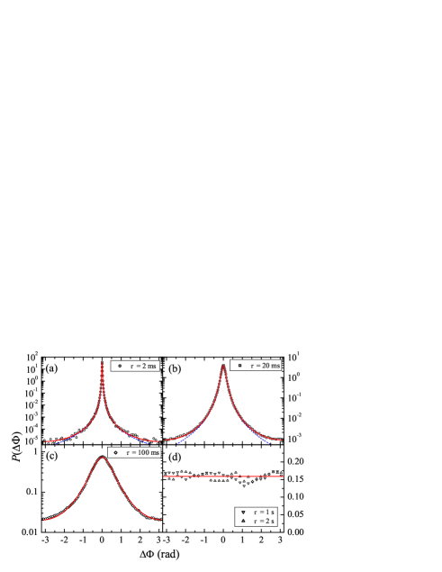
Figure 1: (color online) The observed probability distribution of the wrapped phase evolution at five different time intervals $\tau$ (symbols) and the corresponding theoretical predictions (solid curves). The dashed curves in (a) and (b) are the small $\tau$, small $\Delta\Phi$ predictions (see text). The only fitting parameter (via the dependence of $P(\Delta\Phi)$ on $g_{1})$) is the path phase variance $\langle\Delta\phi_{\mathrm{path}}^{2}\rangle$ at time $\tau$, which gives $\tau_{\mathrm{DAWS}}=89$ ms. For these data, the number of scattering events $n=34\pm 2$. Note the wide variation in vertical scales from (a) to (d).

Figure 1 shows our experimental data for $P(\Delta\Phi)$ at five values of $\tau$, along with fits to Eq. (2). The early times show a narrow peak centered at $\Delta\Phi=0$, which broadens as the particles move further from their original positions. As $\tau$ gets larger, the probability distribution is indeed seen to approach the flat distribution [Fig. 1(d)]. The agreement between theory and experiment is excellent over the entire range of phases and times, and for $P(\Delta\Phi)$ spanning nearly seven orders of magnitude. The fits provide accurate measurements of $\langle\Delta\phi^{2}_{\mathrm{path}}(\tau)\rangle$ and hence of the relative mean square displacement of the particles. Alternatively, by using the universal relationship $\left\langle\Delta\Phi^{2}\right\rangle=f(\langle\Delta\phi^{2}_{\mathrm{path}}\rangle)$ (Fig. 2(a)), $\langle\Delta\phi^{2}_{\mathrm{path}}(\tau)\rangle$ can directly be determined from the measured variance $\left\langle\Delta\Phi^{2}\right\rangle$ - a simpler procedure than fitting $P(\Delta\Phi)$. Both methods work well so long as $\left\langle\Delta\Phi^{2}\right\rangle$ is less than its upper limit of $\pi^{2}/3$ when the phase difference distribution has become flat. In Fig. 2(b), $\left\langle\Delta r^{2}_{\mathrm{rel}}\right\rangle$ measured from the wrapped phase fluctuations and the conventional field autocorrelation are compared. The agreement between the two methods is excellent, giving direct experimental confirmation of the universal relationship shown by the solid curve in Fig 2(a).

In cases where the noise in the measured signals affects the amplitude rather than the phase (eg. gain or DC offset fluctuations), the phase method is more robust for small $\tau$. This is illustrated in the inset to Fig. 2(b), which shows the effect of 2$\%$ random gain fluctuations in the field data; this amplitude noise clearly degrades the measurement of $\langle\Delta r^{2}_{\mathrm{rel}}\rangle$ from $g_{1}$, but does not affect the phase measurement.

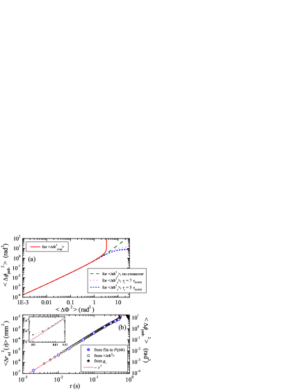
Figure 2: (color online) (a) The universal relationship (solid curve), calculated from Eq. 2, between the variance of the phase shift along one path ($y$-axis), and the measured phase of the transmitted field ($x$-axis). Dashed and dotted lines apply when the phase is unwrapped, making the relation explicitly depend on the motion of the particles. (b) The relative mean square displacement of the particles, $\left\langle\Delta r^{2}_{\mathrm{rel}}(\tau)\right\rangle$ (left axis), determined from the wrapped phase via the corresponding $\langle\Delta\phi_{\mathrm{path}}^{2}\rangle$ (right axis). We compare the results from the wrapped phase shift distribution (${\bigodot}$) and variance ($\square$) with traditional DAWS measurements ($\star$). The inset shows the effect of amplitude noise (see text).

By considering the joint probability distribution of $N=4$ fields in Eq. (1) and by integrating out one phase and four amplitudes, we have obtained an analytic expression for the joint probability distribution of the first three phase derivatives with evolution time $P(\Phi^{\prime},\Phi^{\prime\prime},\Phi^{\prime\prime\prime})$ webpage , from which the individual distribution functions $P(\Phi^{\prime})$, $P(\Phi^{\prime\prime})$ and $P(\Phi^{\prime\prime\prime})$ can be computed. They depend on three parameters $Q,R$ and $S$, that in turn relate to time derivatives of the field correlation function $g_{1}(\tau)$ at $\tau=0$: $Q=-g_{1}^{\prime\prime}(0)$, $R=-[{g_{1}^{(4)}(0)-g_{1}^{\prime\prime}(0)^{2}}]/g_{1}^{\prime\prime}(0)$, and $S=\left[{-g_{1}^{(6)}(0)+\left(g_{1}^{(4)}(0)^{2}/{g_{1}^{\prime\prime}(0)}\right)}\right]/\left[{g_{1}^{(4)}(0)-g_{1}^{\prime\prime}(0)^{2}}\right]$. The fits to the three distributions give the values of $Q$, $S$ and $R$. (Fig. 3). These in turn provide a sensitive probe of the early time behavior of the particle motion, $\langle\Delta r^{2}_{\mathrm{rel}}\rangle$ in powers of $x=\tau/\tau_{\mathrm{DAWS}}$: $\left\langle\Delta r^{2}_{\mathrm{rel}}\right\rangle=324x^{2}-57x^{4}-3.3x^{6}$ $\mu\mathrm{m}^{2}$. We emphasize that, by using this method, details about the motion up to the 6^th power in time can be retrieved, which would be impossible from the conventional DAWS method. Figure 3 also shows that both theoretical and experimental distributions follow an asymptotic power law decay with exponents $-3$, $-2$, $-\frac{5}{3}$ (which suggests $-(1+\frac{2}{n})$ for the $n^{th}$ derivative). These slopes provide a fit-independent test for CGS.

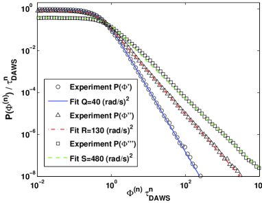
Figure 3: (color online) Comparison of theory and experiment for the phase derivative distribution functions $P(\Phi^{(n)})$, where $n=1,2$ or $3$ denotes the $n^{th}$ derivative of $\Phi$ with respect to evolution time $T$. From $Q$ = 40 rad²/s^-2, we find $\tau_{\mathrm{DAWS}}$ = 91 ms.

To investigate the evolution of the phase over longer times, we study the cumulative (unwrapped) phase $\Phi_{c}(T)$, which can be obtained by adding or subtracting $2\pi$ whenever there is a jump of $\pm 2\pi$ in the wrapped phase. The cumulative phase can be defined as $\Phi_{c}(T)=\int_{0}^{T}\Phi^{\prime}(\tilde{T})\,\mathrm{d}\tilde{T}$, and is, by construction, a continuous random variable that is no longer constrained to the interval $(-\pi,\pi]$. Its ensemble-average vanishes for fields described by CGS. For sufficiently long time intervals, we expect the cumulative phase shift $\Delta\Phi_{c}(\tau)$ to approach the normal distribution with zero mean patrick . Its variance is related to the cumulative phase derivative correlation function, $C_{\Phi^{\prime}}(\tau)\equiv\left\langle\Phi^{\prime}(T-\frac{1}{2}\tau)\Phi^{\prime}(T+\frac{1}{2}\tau)\right\rangle$, which in CGS has the simple analytic form $C_{\Phi^{\prime}}(\tau)=\frac{1}{2}(\ln g_{1})^{\prime\prime}\ln(1-g_{1}^{2})$ anacheEPL . Fig. 4(a) compares theory and experiment for $C_{\Phi^{\prime}}$, where predictions based on a simple empirical crossover model for the particle dynamics are also included daws , for which $\left\langle\Delta r^{2}_{\mathrm{rel}}(\tau)\right\rangle=\left\langle\Delta V^{2}_{\mathrm{rel}}\right\rangle\tau^{2}/\left(1+\tau^{2}/\tau_{c}^{2}\right)$. The best fit is obtained for $\tau_{c}=7\tau_{\mathrm{DAWS}}$, showing that both $\tau_{\mathrm{DAWS}}$ and $\tau_{c}$ can be determined from $C_{\Phi^{\prime}}$.

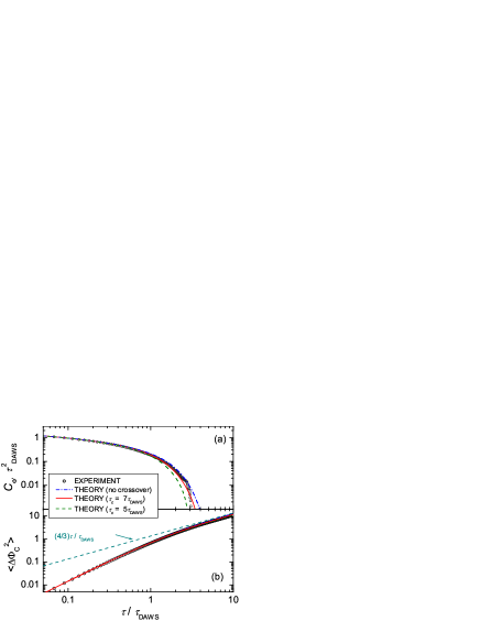
Figure 4: (color online) Comparison of theory and experiment for (a) the phase derivative correlation function $C_{\Phi^{\prime}}$, (b) the cumulative phase shift variance $\left\langle\Delta\Phi^{2}_{c}(\tau)\right\rangle$.

The cumulative phase shift variance can be calculated from $C_{\Phi^{\prime}}$ since $\left\langle\Delta\Phi^{2}_{c}(\tau)\right\rangle=2\int_{0}^{\tau}d\nu(\tau-\nu)C_{\Phi^{\prime}}(\nu)$ anacheEPL . Recalling the expression for $C_{\Phi^{\prime}}(\tau)$ reveals that the variance of cumulative phase evolution is determined by $g_{1}$ and its first two derivatives. This destroys the universal relation with the path phase variance, but at the same time this increases the sensitivity to details in particle motion at long times (see Fig. 2(a)). At short times, the cumulative phase variance increases as a power law with a logarithmic correction, $\left\langle\Delta\Phi^{2}_{c}(\tau)\right\rangle=\frac{1}{3}\tau^{2}/\tau_{\mathrm{DAWS}}^{2}[1.5-\ln(\tau/\sqrt{3}\,\tau_{\mathrm{DAWS}})]$, while at long times, the cumulative phase shift evolves as a 1D random process with finite diffusion constant: $\left\langle\Delta\Phi^{2}_{c}(\tau)\right\rangle\rightarrow D_{\Delta\Phi}\,\tau$ (Fig. 4(b)). For $\tau_{c}\gg\tau_{\mathrm{DAWS}}$, we find $D_{\Delta\Phi}=\frac{4}{3}\tau_{\mathrm{DAWS}}$. The cumulative phase variance is quite different from the path phase variance $\langle\Delta\phi_{\mathrm{path}}^{2}\rangle$, which has a finite diffusion constant only if the particles undergo Brownian motion, which they do not here. By comparing measured and theoretical $\left\langle\Delta\Phi_{c}^{2}(\tau)\right\rangle$ in Fig. 4(b), the accurate value of $\tau_{\mathrm{DAWS}}=89$ ms was deduced from an appropriate translation along the $x$ direction.

We have studied the phase evolution of ultrasonic waves in strongly scattering, dynamic media. It is important to discriminate the random phase evolution along one scattering path, usually studied in D(A)WS, from the observed phase evolution in a single speckle spot. Our experiments are extremely well modelled by circular Gaussian statistics. This theory accurately predicts the behavior of the wrapped phase difference probability distribution, the variance of both the wrapped and cumulative phase shifts, and the phase derivative distributions and correlation function. The excellent agreement of theory and experiment has allowed us to relate the observed fluctuations in phase evolution to the relative mean square displacement of the scatterers. The phase statistics are sensitive probes of the particle motion on both short and long time scales, and can provide more accurate information than the more traditional field fluctuation measurements.

We wish to thank NSERC for its support, and T. Norisuye for assisting with some of the data analysis.

References

- (1) For a review see: R. Berkovits and S. Feng, Phys. Rep. 238, 135 (1994); A.Z. Genack in: Scattering and Localization of Classical waves in Random Media, edited by Ping Sheng (World Scientific, Singapore, 1990).
- (2) Wave Scattering in Complex Media, edited by B.A. van Tiggelen and S.E. Skipetrov (Kluwer, Dordrecht 2003)
- (3) P.A. Lee and A.D. Stone, Phys. Rev. Lett. 55, 1622 (1986).
- (4) S. Feng et al., Phys. Rev. Lett. 61, 834 (1988); F. Scheffold and G. Maret, Phys. Rev. Lett. 81, 5800 (1998).
- (5) A.A. Chabanov et al., Phys. Rev. Lett. 92, 173901 (2004).
- (6) G. Maret, and P.E. Wolf, Z. Phys. B. 65, 409 (1987); D.J. Pine, D.A. Weitz, P.M. Chaikin and E. Herbolzheimer, Phys. Rev. Lett. 60, 1134 (1988).
- (7) M.L. Cowan et al., Phys. Rev. Lett. 85, 453 (2000); M.L. Cowan et al., Phys. Rev. E 65, 066605 (2002).
- (8) R. Snieder et al., Science 295, 22553 (2002).
- (9) C. Wicks et al., Science 282, 458 (1998) ; C. Wicks et al., Nature 440, 72 (2006).
- (10) M.V. Berry and M.R. Dennis, Proc. R. Soc. London Ser. A 456 2059 (2000); I. Freund and M. Wilkinson, J.Opt.Soc. Am. A 15, 2892 (1998); M. Wilkinson J. Phys. A: Math Gen. 37, 6763 (2004).
- (11) A.Z. Genack et al., Phys. Rev. Lett. 82, 715 (1999); B.A. van Tiggelen et al., Phys. Rev. E 59, 7166 (1999); A.Z. Genack et al. in Ref. book ; A.A. Chabanov and A.Z. Genack, Phys. Rev. Lett. 87, 233903 (2001); H. Schomerus, Phys. Rev. E 64, 026606 (2001).
- (12) I. M. Vellekoop, P. Lodahl, and A. Lagendijk, Phys. Rev. E 71, 056604 (2005).
- (13) J. Pearce, Z. Jian, and D. M. Mittleman, Phys. Rev. Lett. 91, 043903 (2003)
- (14) J.H. Page et al. in Ref. book , p. 151.
- (15) J.W. Goodman, Statistical Optics (Wiley, N.Y., 1985).
- (16) Since our samples do not undergo any uniform dilation, such as could arise from changes in wave velocity due to temperature changes, the average phase is zero, and the variance characterizes the dynamics.
- (17) See EPAPS Document No. [ ] for formulae. This document can be reached through a direct link in the online article’s HTML reference section or via the EPAPS homepage (http://www.aip.org/pubservs/epaps.html).
- (18) P. Sebbah et al., Phys. Rev. E 56, 3619 (1997).
- (19) B.A. van Tiggelen, D. Anache and A. Ghysels, Europhys. Lett. 74, 999 (2006).