Central limit behavior of deterministic dynamical systems

Abstract

We investigate the probability density of rescaled sums of iterates of deterministic dynamical systems, a problem relevant for many complex physical systems consisting of dependent random variables. A Central Limit Theorem (CLT) is only valid if the dynamical system under consideration is sufficiently mixing. For the fully developed logistic map and a cubic map we analytically calculate the leading-order corrections to the CLT if only a finite number of iterates is added and rescaled, and find excellent agreement with numerical experiments. At the critical point of period doubling accumulation, a CLT is not valid anymore due to strong temporal correlations between the iterates. Nevertheless, we provide numerical evidence that in this case the probability density converges to a $q$-Gaussian, thus leading to a power-law generalization of the CLT. The above behavior is universal and independent of the order of the maximum of the map considered, i.e. relevant for large classes of critical dynamical systems.

The Central Limit Theorem (CLT) is an extremely important concept in probability theory and it also lies at the heart of statistical physics vKa ; khinchin . It basically says that the sum of $N$ independent identically distributed (IID) random variables, rescaled with a factor $1/\sqrt{N}$, has a Gaussian distribution in the limit $N\to\infty$. The CLT plays a crucial role in explaining why many stochastic processes that are of relevance in physics, chemistry, biology, economics, etc. are Gaussian, provided they consist of a sum of many independent or nearly independent contributions. CLTs are also of fundamental importance to ‘derive’ statistical mechanics from first principles: If a CLT is valid for the driving forces in a many-body system, it is easy to proceed to the formalism of statistical mechanics via the Langevin and Fokker-Planck approaches.

What is less known in the physics community but well-known in the mathematics community is the fact that there are also CLTs for the iterates of deterministic dynamical systems. The iterates of a deterministic dynamical system can never be completely independent, since they are generated by a deterministic algorithm. However, if the assumption of IID is replaced by the weaker property that the dynamical system is sufficiently strongly mixing, then various versions of CLTs can be proved for deterministic dynamical systems bill ; kac ; chernov ; keller ; beck ; roep ; michael . It should be kept in mind that the mixing property just means asymptotic statistical independence for large time differences.

In this letter we investigate in detail the central limit behavior of deterministic systems. We are interested in two questions that are of fundamental importance for the foundations of statistical mechanics: a) Suppose a CLT is valid for a deterministic dynamical system for $N\to\infty$, what are the leading-order corrections to the CLT for large but finite $N$? b) Suppose the dynamical system does not satisfy a CLT because it is not sufficiently mixing, what are typical probability distributions that one obtains for these types of systems in the limit $N\to\infty$?

The above questions are very relevant to understand the physics of complex systems in general. First of all, any physical system always consists of a finite number $N$ of constituents rather than an infinite one. Hence finite-$N$ corrections to the CLT can be potentially important for small systems. Secondly, the dynamics of critical systems usually exhibits strong correlations. These imply that an ordinary CLT cannot be valid. In such cases it is important to know what type of distributions replace the usual Gaussian limit distributions.

In full generality, the above two problems are very difficult to deal with. Hence there is the need to start with simple model systems where some statements can be rigorously proved. Our main example in the following is the logistic map. For the fully developed chaotic state of this map, a CLT has been proved bill . We will explicitly calculate leading-order corrections to the Gaussian limit case if a finite number $N$ of iterates is added and rescaled with $1/\sqrt{N}$. Moreover, we will provide evidence that at the critical point of period doubling accumulation, where a CLT is not valid due to strong correlations between the iterates, a suitably rescaled sum of iterates appears to generate distributions with power law tails, which are well approximated by $q$-Gaussians. These distributions are known to play an important role in generalized versions of statistical mechanics tsa1 ; tsa2 ; tsa3 . Although our results are derived for the special example of the logistic map, we will show that they are universal, i.e., applicable to entire classes of deterministic dynamical systems.

To start with, let us consider a $d$-dimensional mapping of the form

$$x_{i+1}=T(x_{i})$$ (1)

on some $d$-dimensional phase space $X$. If $T$ is sufficiently strongly mixing (see bill ; roep ; chernov ; michael for technical details), one can prove the existence of a CLT. This means the probability distribution of

$$y:=\frac{1}{\sqrt{N}}\sum_{i=1}^{N}f(x_{i}),$$ (2)

becomes Gaussian for $N\to\infty$, regarding the initial value $x_{1}$ as a random variable. Here $f:{\cal R}^{d}\to{\cal R}^{k}$ is a suitable smooth function with vanishing average which projects from the $d$-dimensional phase space to a $k$-dimensional subspace. If $d=k=1$, the variance $\sigma^{2}$ of this Gaussian is given by roep

$$\sigma^{2}=\langle f(x_{0})^{2}\rangle+2\sum_{i=1}^{\infty}\langle f(x_{0})f(x_{i})\rangle.$$ (3)

Here $\langle\cdots\rangle$ denotes an expectation formed with the natural invariant density of the map $T$.

Figure 1: (Color online) Probability density of rescaled sums of iterates of the logistic map with $a=2$ as given by eq. (8), $N=2\times 10^{6}$ and $N=100$. The number of initial values contributing to the histogram is $n_{ini}=2\times 10^{6}$, respectively $n_{ini}=10^{7}$. The solid lines correspond to eq. (9).

As an example to illustrate these general results, let us consider the logistic map

$$x_{i+1}=T(x_{i})=1-ax_{i}^{2}$$ (4)

on the interval $X=[-1,1]$. For $a=2$ the system is (semi)conjugated to a Bernoulli shift and strongly mixing. The natural invariant density is

$$\rho_{x}(x)=\frac{1}{\pi\sqrt{1-x^{2}}}.$$ (5)

Ergodic averages of arbitrary observables $A$ are given by

$$\langle A(x)\rangle=\int_{-1}^{1}\rho(x)A(x)dx.$$ (6)

The average $\langle x\rangle$ vanishes. For the correlation function one has

$$\langle x_{i_{1}}x_{i_{2}}\rangle=\frac{1}{2}\delta_{i_{1},i_{2}}.$$ (7)

Due to the strong mixing property, the conditions for the validity of a CLT are satisfied for $a=2$. This means the distribution of the quantity

$$y:=\frac{1}{\sqrt{N}}\sum_{i=1}^{N}(x_{i}-\langle x\rangle)$$ (8)

becomes Gaussian for $N\to\infty$, regarding the initial value $x_{1}$ as a random variable with a smooth probability distribution. For the variance of this Gaussian we obtain from eq. (3) and (7) the value $\sigma^{2}=\frac{1}{2}$ (choosing $f(x)=x$). The above CLT result is highly nontrivial, since there are complicated higher-order correlations between the iterates of the logistic map for $a=2$ (see nonli for details). This means the ordinary CLT, which is only valid for independent $x_{i}$ cannot be directly applied, an extension of the CLT for mixing systems is necessary bill .

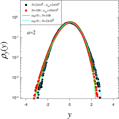
For physical and practical applications, the number $N$ is always finite, hence it is important to know what the finite-$N$ corrections are for a given dynamical system. This problem can be solved for our example, the map $T(x)=1-2x^{2}$, by applying the general graph-theoretical methods developed in nonli ; hilgers . Our final result is that for finite but large $N$ the probability density of $y$ is given by

$$\rho_{y}(y)=\frac{1}{\sqrt{\pi}}e^{-y^{2}}\Big{[}1+\frac{1}{\sqrt{N}}y\left(\frac{3}{2}-y^{2}\right)+O\left(\frac{1}{N}\right)\Big{]}.$$ (9)

This result is in excellent agreement with numerical experiments (Fig. 1).

Figure 2: (Color online) Probability density of rescaled sums of iterates of the cubic map (10) for $N=10^{7}$ and $N=10$. The number of initial values is $n_{ini}=10^{6}$, respectively $n_{ini}=5\times 10^{6}$. The solid lines correspond to eq. (11).

We should mention at this point that the finite-$N$ corrections are non-universal, i.e. different mappings have different finite-$N$ corrections. For example, by applying the techniques of nonli ; hilgers to the cubic map

$$x_{i+1}=4x_{i}^{3}-3x_{i},$$ (10)

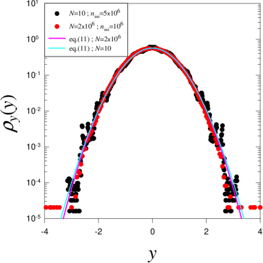
which has the same invariant density (5) as the logistic map with $a=2$ but different higher-order correlations, we obtain in leading order

$$\rho_{y}(y)=\frac{1}{\sqrt{\pi}}e^{-y^{2}}\Big{[}1+\frac{1}{N}\left(\frac{1}{12}y^{4}-\frac{1}{4}y^{2}+\frac{1}{16}\right)\Big{]}.$$ (11)

Note that in this case the leading-order corrections are of order $1/N$, rather than of order $1/\sqrt{N}$. Again our analytical result is in good agreement with the numerics, see Fig. 2.

Apparently the finite-$N$ corrections to the asymptotic Gaussian behavior of dynamical systems satisfying a CLT are non-universal and can be used to obtain more information on the underlying deterministic dynamics. This is certainly important from a general physical point of view if the dynamics underlying a CLT is a priori unknown.

We may also look at distributions of the variable $y$ obtained for ‘typical’ parameter values in the chaotic regime of the logistic map, such as $a=1.7,1.8,1.9$. A CLT has not been rigorously proved in this case, but nevertheless we again observe Gaussian limit behavior. This is shown in Fig. 3. It is a well-known fact that for $a<2$ the average $\langle x\rangle$ does not vanish anymore. The Gaussians observed in Fig. 3 have smaller variance $\sigma^{2}$ as compared to the case $a=2$. This can be understood in a quantitative way from eq. (3). The fits in Fig. 3 show Gaussians with variance parameter $\sigma^{2}$ directly determined from eq. (3) using $f(x)=x-\langle x\rangle$ (the averages $\langle\dots\rangle$ are calculated as time averages). Note that for $a=1.7,1.8,1.9$ the correlation function is not $\delta$-correlated anymore.

Figure 3: (Color online) Probability density of rescaled sums of iterates of the logistic map as given by eq. (8) for $a=1.7,1.8,1.9$ and $N=2\times 10^{6}$, $n_{ini}=10^{6}$. The solid lines show Gaussians $e^{-y^{2}/(2\sigma^{2})}/\sqrt{2\pi\sigma^{2}}$ with variance parameter $\sigma^{2}$ determined from eq. (3).

Next, let us investigate the behavior of deterministic dynamical systems where the conditions for a CLT are not satisfied. As a particularly interesting example, we choose the logistic map at the accumulation point of period doublings (i.e., at the edge of chaos). The corresponding parameter value is denoted by $a_{c}$. For $a=a_{c}$ the logistic map is not sufficiently strongly mixing and a CLT is not valid. Still one can ask the question if there is a universal limit distribution for suitably rescaled sums of iterates. We investigated this question numerically and looked at rescaled sums of the form

$$y=N^{\gamma}\sum_{i=1}^{N}(x_{i}-\langle x\rangle).$$ (12)

Eq. (12) is a generalization of eq. (8) with a more general rescaling exponent $\gamma$. The notation $\langle\cdots\rangle$ means an average over a large number $N$ of iterations and a large number $n_{ini}$ of randomly chosen initial values $x_{1}^{(j)}$. Numerically we calculate

$$\langle x\rangle=\frac{1}{n_{ini}}\frac{1}{N}\sum_{j=1}^{n_{ini}}\sum_{i=1}^{N}x_{i}^{(j)}.$$ (13)

Due to the fact that the system is not necessarily ergodic anymore, the average over initial conditions is an important ingredient.

Figure 4: (Color online) Probability density of the quantity $y/\sigma$ at the critical point $a_{c}$ for $z=2$, $N=2^{14}$ and $N=2^{15}$.

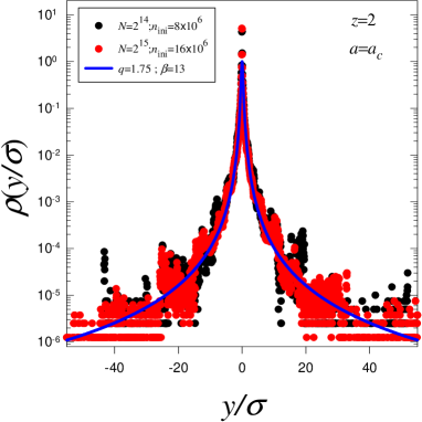
In our numerical experiment, a large number of initial values $x_{1}$ were randomly chosen and the corresponding values of the sum $Y$ were plotted in a histogram. We then looked for a suitable rescaling exponent $\gamma$ where we have data collapse, i.e., the same shape of the probability distributions $\rho_{y}(y)$ of $y$ if $N$ is increased. Numerically we observe that, at $a=a_{c}$, this value is given by $\gamma=1.5$. The density of $y$ is not given by a Gaussian, as one would expect if a CLT is valid, but well fitted by a $q$-Gaussian, i.e. a distribution of the form

$$\rho_{y}(y)\sim e_{q}^{-\beta y^{2}}:=\frac{1}{(1+\beta(q-1)y^{2})^{\frac{1}{q-1}}},$$ (14)

where $q$ and $\beta$ are suitable parameters. We observe $q=1.75\pm 0.03$ (see Fig. 4). The rescaling factor $N^{\gamma}$ in eq. (12) can be absorbed by simply calculating the variance $\sigma^{2}$ of the unrescaled sum $y:=\sum_{i=1}^{N}(x_{i}-\langle x\rangle)$ for a given $N$ and then plotting a histogram of $y/\sigma$.

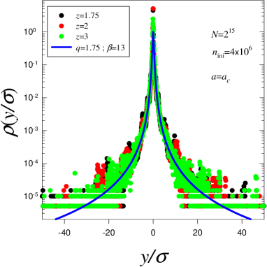
Interesting enough, the values of $q$ and $\gamma$ that we observe in our numerical experiments are independent of the order of the maximum of the map considered. Indeed, if instead of the logistic map (4) we iterate the more general map

$$x_{i+1}=1-a|x_{i}|^{z},$$ (15)

then at the critical point $a_{c}(z)$ of period doubling accumulation the results are basically unchanged (see Fig. 5).

Since at the critical point the dynamics of many different maps converges to a dynamics given by the universal Feigenbaum fixed point function fei , our results for the asymptotic probability distribution of $Y$ are universal: Entire classes of critical quadratic maps will generate the same $q$-Gaussian limit distribution. Our result is even more universal since there seems to be no dependence on the order $z$ of the maximum of the map. Thus we expect the $q$-Gaussian limit distribution with $q\approx 1.75$ to be relevant for many different dynamical systems at the critical point.

The independence of $z$ has also been established in a different context: In robledo2004 it is shown that, for all values of $z$, the relevant fixed point map describing period doubling bifurcations (tangent bifurcations) is a specific $q$-exponential with $q=3$ ($q=2$).

Figure 5: (Color online) Probability density of the quantity $y/\sigma$ at the critical point $a_{c}$ for $z=1.75,2,3$.

The generalized central limit behavior of critical dynamical systems observed in this paper may be of relevance for more general classes of critical systems in physics as well. For example, Caruso et al. rapi observe that the probability distribution of energy differences of subsequent earthquakes in the World Catalog and in Northern California is well fitted by a $q$-Gaussian with $q\approx 1.75$. Their model for this is based on self-organized criticality and the OFC model. We note that $q$-Gaussians with $q\approx 1.75$ arise naturally if the corresponding random variable consist of a sum of strongly correlated contributions as generated by critical dynamical systems. A somewhat similar result has also been recently observed for Brazilian financial data: A $q$-Gaussian with $q\simeq 1.75$ fits histograms of stock market index changes for a considerable range of time delays (see Fig. 6 of cortines ).

To conclude, in this paper we have explicitly calculated finite-$N$-corrections to the CLT for some examples of strongly mixing dynamical systems. For critical systems at the edge of chaos, where a CLT is not valid anymore due to strong correlations, we have shown that the relevant limit distributions appear to be $q$-Gaussians with $q\approx 1.75$. This result is universal and independent of the order of the maximum of the map under consideration. Our results represent a kind of power-law generalization of the CLT, which is relevant for entire classes of dynamical systems. An analytical study of the present results at the edge of chaos and of more general critical dynamical systems would be very welcome. This might, in particular, enlighten the deep reasons for the frequent occurrence of $q$-Gaussians in natural, artificial and social complex systems.

This work has been supported by TUBITAK (Turkish Agency) under the Research Project number 104T148. C.B. acknowledges financial support by EPSRC. C.T. acknowledges partial financial support from Pronex, CNPq and Faperj (Brazilian Agencies).

References

- (1) N.G. van Kampen, Stochastic Processes in Physics and Chemistry, North Holland, Amsterdam (1981)
- (2) A.Ya. Khinchin, Mathematical Foundations of Statistical Mechanics, Dover, New York (1949)
- (3) P. Billingsley, Convergence of Probability Measures, Wiley, New York (1968)
- (4) M. Kac, Ann. Math. 47, 33 (1946)
- (5) N.I. Chernov, Prob. Theor. Rel. Fields 101, 321 (1995)
- (6) F. Hofbauer and G. Keller, Math. Z. 180, 119 (1982)
- (7) C. Beck, Physica A 169, 324 (1990)
- (8) C. Beck and G. Roepstorff, Physica A 145, 1 (1987)
- (9) M.C. Mackey and M. Tyran-Kaminska, Phys. Rep. 422, 167 (2006)
- (10) C. Tsallis, J. Stat. Phys. 52, 479 (1988)
- (11) C. Tsallis, Physica A 365, 7 (2006)
- (12) S. Umarov, C. Tsallis, and S. Steinberg, cond-mat/0603593; see also S. Umarov, C. Tsallis, M. Gell-Mann and S. Steinberg, cond-mat/0606038 and cond-mat/0606040.
- (13) C. Beck, Nonlinearity 4, 1131 (1991)
- (14) A. Hilgers and C. Beck, Physica D 156, 1 (2001)
- (15) M.J. Feigenbaum, J. Stat. Phys. 46, 919 (1987)
- (16) A. Robledo, Physica D 193, 153 (2004).
- (17) F. Caruso, A. Pluchino, V. Latora, S. Vinciguerra, and A. Rapisarda, cond-mat/0606118.
- (18) A.A.G. Cortines and R. Riera, Physica A 377, 181(2007).