Spin-Hall effect and spin-coherent excitations in a strongly confined two-dimensional hole gas

Abstract

Based on a rigorous quantum-kinetic approach, spin-charge coupled drift-diffusion equations are derived for a strongly confined two-dimensional hole gas. An electric field leads to a coupling between the spin and charge degrees of freedom. For weak spin-orbit interaction, this coupling gives rise to the intrinsic spin-Hall effect. There exists a threshold value of the spin-orbit coupling constant that separates spin diffusion from ballistic spin transport. In the latter regime, undamped spin-coherent oscillations are observed. This result is confirmed by an exact microscopic approach valid in the ballistic regime.

The generation and manipulation of a spin polarization by exclusively electronic means in nonmagnetic semiconductors at room temperature is a major challenge of spintronics. Among many interesting phenomena, the intrinsic spin-Hall effect (SHE) SCIE_1348 ; PRL_126603 has recently attracted considerable interest. Experimental studies SCIE_1910 ; PRL_047204 ; PRL_096605 reveal an electric-field induced spin accumulation near the edges of a confined two-dimensional electron (hole) gas. Most theoretical interpretations of these experimental data rely on the notion of a spin current oriented transverse to the applied electric field. SCIE_1348 ; PRL_126603 Interestingly, this seemingly clear physical picture still remains the subject of serious debates.PRL_076604 ; PRB_165313 The relationship between the spin current and the induced spin polarization seems to be a very subtle issue. The main problem underlying the debates is the notion of a spin current itself because spin is not a conserved quantity in spin-orbit coupled systems. Consequently, any approach that avoids the intricate identification of a more or less suitable spin current is superior. Such an alternative approach not only introduces different calculational techniques, but also suggests alternative interpretations of the effects under consideration. As widely anticipated, a complete physical description of spin-related phenomena is provided by microscopic models based on the spin-density matrix or Keldysh Green functions together with an analysis of its long-wavelength and low-frequency limit. These approaches are more general and free from artefact associated with ambiguous definitions of the spin current. In addition, spin-charge coupled kinetic equations allow the treatment of such interesting phenomena as propagating spin excitations or the relationship between the intrinsic SHE and the zitterbewegung.

In this report, we propose an alternative approach to the SHE by deriving spin-charge coupled drift-diffusion equations for a two-dimensional hole gas (2DHG), which refers to the populated heavy-hole band of thin p-type quantum wells. The related heavy-hole Hamiltonian of the cubic Rashba model has the second quantized form

$$H=\sum_{{\bm{k}},\lambda}a_{\bm{k}\lambda}^{{\dagger}}\left[\varepsilon_{\bm{k}}-\varepsilon_{F}\right]a_{\bm{k}\lambda}-\sum_{\bm{k},\lambda,\lambda^{\prime}}\left(\hbar{\bm{\omega}}_{\bm{k}}\cdot{\bm{\sigma}}_{\lambda\lambda^{\prime}}\right)a_{\bm{k}\lambda}^{{\dagger}}a_{\bm{k}\lambda^{\prime}}$$

$$+u\sum\limits_{{\bm{k}},{\bm{k}}^{\prime}}\sum\limits_{\lambda}a_{{\bm{k}}\lambda}^{{\dagger}}a_{{\bm{k}}^{\prime}\lambda}-ie{\bm{E}}\sum\limits_{{\bm{k}},\lambda}\nabla_{\bm{\kappa}}a^{{\dagger}}_{{\bm{k}}-{\bm{\kappa}}/2\lambda}a_{{\bm{k}}+{\bm{\kappa}}/2\lambda}\mid_{\bm{\kappa}=0},$$ (1)

where $a_{\bm{k}\lambda}^{{\dagger}}$ ($a_{\bm{k}\lambda}$) denote the creation (annihilation) operators with in-plane quasi-momentum $\bm{k}=(k_{x},k_{y},0)$ and spin $\lambda$. The electric field ${\bm{E}}$ is oriented along the $x$ axis. Furthermore, $\varepsilon_{F}$ denotes the Fermi energy, $\bm{\sigma}$ the vector of Pauli matrices, $\varepsilon_{\bm{k}}=\hbar^{2}k^{2}/(2m)$, and $u$ the strength of the ’white-noise’ elastic impurity scattering, which gives rise to the momentum relaxation time $\tau$. Contrary to a phenomenological approach, we treat elastic scattering on a full microscopic scope. The spin-orbit coupling is given by

$$\hbar{\bm{\omega}}_{\bm{k}}=\frac{\alpha}{2}\left[i(k_{+}^{3}-k_{-}^{3}),(k_{+}^{3}+k_{-}^{3}),0\right],$$ (2)

where $k_{\pm}=k_{x}\pm ik_{y}$ and $\hbar\omega_{k}=\alpha k^{3}$. Based on the Born approximation for elastic impurity scattering, the Laplace-transformed kinetic equations for the physical components of the spin-density matrix have the form PRB_165313

$$sf-\frac{i\hbar}{m}(\bm{\kappa}\cdot\bm{k})f+i{\bm{\omega}}_{\bm{\kappa}}({\bm{k}})\cdot{\bm{f}}+\frac{e{\bm{E}}}{\hbar}\nabla_{\bm{k}}f=\frac{1}{\tau}(\overline{f}-f)+f_{0},$$ (3)

$$s{\bm{f}}+2({\bm{\omega}}_{\bm{k}}\times{\bm{f}})-\frac{i\hbar}{m}(\bm{\kappa}\cdot\bm{k}){\bm{f}}+i{\bm{\omega}}_{\bm{\kappa}}({\bm{k}})f+\frac{e{\bm{E}}}{\hbar}\nabla_{\bm{k}}{\bm{f}}$$

$$=\frac{1}{\tau}(\overline{{\bm{f}}}-{\bm{f}})+\frac{1}{\tau}\frac{\partial}{\partial\varepsilon_{\bm{k}}}\overline{f\hbar{\bm{\omega}}_{\bm{k}}}-\frac{\hbar{\bm{\omega}}_{\bm{k}}}{\tau}\frac{\partial}{\partial\varepsilon_{\bm{k}}}\overline{f}+{\bm{f}}_{0},$$ (4)

where an additional frequency appears

$${\bm{\omega}}_{\bm{\kappa}}({\bm{k}}) = \frac{3\alpha}{\hbar}\left[(k_{y}^{2}-k_{x}^{2})\kappa_{y}-2k_{x}k_{y}\kappa_{x},\right.$$ (5)

$$\left.(k_{x}^{2}-k_{y}^{2})\kappa_{x}-2k_{x}k_{y}\kappa_{y},0\right],$$

which depends on ${\bm{\kappa}}$. The cross line over ${\bm{k}}$-dependent quantities denotes an integration over the polar angle $\varphi$ of the in-plane vector ${\bm{k}}$. $f_{0}$ and ${\bm{f}}_{0}$ denote the initial charge and spin density components, respectively. The quantum Boltzmann equations (3) and (4) are treated in the long-wavelength limit in order to derive spin-charge coupled drift-diffusion equations. To this end, the kinetic equations are written in a matrix form $A\widehat{f}+{\cal E}\widehat{f}=B\overline{\widehat{f}}+\widehat{\delta}$, where the matrix $A$ collects all contributions that are independent of the electric field ${\bm{E}}$ and not integrated over the angle $\varphi$ [$\widehat{f}$ denotes the four component vector $(f,{\bm{f}})$]. To calculate the matrix $B$ on the right-hand side of this equation, we assume $\alpha k_{F}^{3}\ll\varepsilon_{k_{F}}$ and restrict $\kappa$ contributions up to $\kappa^{2}$. The matrix equation is solved iteratively in the case of weak electric field contributions ${\cal E}$ (the matrix ${\cal E}$ contains first-order derivatives and $\widehat{f}$ is decomposed according to $\widehat{f}_{0}+\widehat{f}_{1}$ with $\widehat{f}_{0}\sim E^{0}$ and $\widehat{f}_{1}\sim E$). The solution of the equation is written in the form

$$(1+\overline{C}_{1}^{-1}\overline{C}_{2})^{-1}\overline{C}_{1}^{-1}\overline{\widehat{f}}=\widehat{\delta},$$ (6)

where $\overline{\widehat{f}}_{0}=\overline{C}_{1}\widehat{\delta}$ and $\overline{\widehat{f}}_{1}=\overline{C}_{2}\widehat{\delta}$. The general expressions for the transport coefficients are very cumbersome but simplify considerably in the low-field case and under the condition $\alpha k_{F}^{3}\ll\varepsilon_{k_{F}}$.

As we are mainly interested in the SHE, let us focus on the coupling between the spin and charge degrees of freedom. By applying the outlined schema, we obtain our main analytical result

$$(s+i\frac{v_{d}}{\sigma_{0}}\kappa_{x}+D_{0}\kappa^{2})\overline{f}+i\Gamma_{z}\kappa_{y}\overline{f}_{z}=f_{0},$$ (7)

$$(s+\frac{1}{\tau_{sz}}+i\frac{v_{d}}{\sigma_{0}}\kappa_{x}+D_{z}\kappa^{2})\overline{f}_{z}+i\Gamma_{0}\kappa_{y}\overline{f}=0,$$ (8)

with the transport coefficients

$$D_{0}=\frac{D}{\sigma_{0}^{2}},\quad D_{z}=D\frac{\sigma_{0}^{2}-12\Omega^{2}}{(\sigma_{0}^{2}+4\Omega^{2})^{2}},$$ (9)

$$\Gamma_{0}=v_{d}\frac{9\Omega^{2}}{2\gamma}\frac{3\sigma_{0}^{2}-4\Omega^{2}}{(\sigma_{0}^{2}+4\Omega^{2})^{2}},\quad\frac{1}{\tau_{sz}}=\frac{4\Omega^{2}}{\sigma_{0}\tau},$$ (10)

$$\Gamma_{z}=v_{d}\frac{9\Omega^{2}}{2\gamma}\sigma_{0}^{2}\frac{4\sigma_{0}\Omega^{2}+8\Omega^{2}-3\sigma_{0}^{2}s\tau}{(\sigma_{0}s\tau+4\Omega^{2})(\sigma_{0}^{2}+4\Omega^{2})}.$$ (11)

The parameters introduced in these equations are given by: $v_{d}=eE\tau/m$, $\sigma_{0}=s\tau+1$, $D=v^{2}\tau/2$, $\gamma=\varepsilon_{k}\tau/\hbar$, and $\Omega=\omega_{k}\tau=K(k)l$ (with $K(k)=\alpha mk^{2}/\hbar^{2}$ and the mean-free path $l=v\tau$). As the contributions $\sim\kappa_{x}$ do not affect our analysis, we took them to lowest order in $\Omega$. The Eqs. (7) and (8) have been derived for $\Omega/\gamma\ll 1$ but unrestricted values $\Omega$. In the absence of the electric field ($E=0$), the Eqs. (7) and (8) completely decouple. This decoupling, which applies to all components of the spin-density matrix, represents a speciality of the cubic Rashba model. PRB_193316 ; PRB_195330 The situation is completely different for electrons (linear Rashba model), for which at zero external fields the charge density $\overline{f}$ couples to the transverse spin component $\overline{f}_{r}=i({\bm{\kappa}}\times{\overline{\bm{f}}})_{z}$, whereas $\overline{f}_{z}$ is connected with the longitudinal component $\overline{f}_{d}=i{\bm{\kappa}}\cdot{\overline{\bm{f}}}$. However, both for the linear and cubic Rashba model additional couplings arise due to an applied electric field. The related magnetization gives rise to a magnetoelectric effect that has been thoroughly investigated in the literature for semiconductors with spin-orbit interaction.

The time dependence of the coupled spin-charge transport is calculated by an inverse Laplace transformation of the solution of Eqs. (7) and (8). Due to the complicated $s$ dependence of all transport coefficients, a non-Markovian temporal evolution is expected. However, the straightforward determination of this complicated time dependence of charge and spin densities becomes problematic. Eqs. (7) and (8) are only solvable by inverse Fourier- and Laplace transformations under appropriate additional approximations concerning the $s$ dependence. This delicate mathematical problem will be accounted for in a forthcoming paper. Here, we focus on steady-state solutions ($\sigma_{0}=1$).

The character of the coupled spin-charge transport strongly depends on the strength of the spin-orbit coupling, which is expressed by the dimensionless parameter $\Omega=K(k)l$. It is the most striking feature of the drift-diffusion Eqs. (7) and (8) that the character of the spin transport changes radically with increasing coupling strength $\Omega$. The appearance of such a crossover is due to the unusual expression for the diffusion coefficient $D_{z}$ in Eq. (9), which has recently been derived by an alternative approach. PRB_193316 Moreover, the very same result is also obtained for the linear Rashba model, when the frequency $\omega_{k}$ is appropriately redefined. With increasing spin-orbit coupling $K(k)$ or relaxation time $\tau$, the diffusion coefficient $D_{z}$ changes its sign. A negative diffusion coefficient indicates an instability of the spin system. Under this condition, spin diffusion has the tendency to strengthen initial spin fluctuations. The competition between this self strengthening and spin relaxation processes results in a spatial oscillatory spin pattern. Going from weak ($\Omega<1/\sqrt{12}$) to strong ($\Omega>1/\sqrt{12}$) spin-orbit coupling, we observe a transition in the spin system from a diffusive behavior to a ballistic regime. We shall show that ballistic spin transport is characterized by undamped spin oscillations.

To be specific, let us solve Eqs. (7) and (8) for a stripe geometry ($-L_{0}\leq y\leq L_{0}$). The inverse Fourier transformation is accomplished by the replacement $\kappa_{y}\rightarrow i\partial/\partial y$, whereas along the $x$ axis all quantities are constant. The resulting set of differential equations is easily solved. For the boundary condition $\overline{f}(-L_{0})=\overline{f}(L_{0})=f_{0}$ and $\overline{f}_{z}(-L_{0})=\overline{f}_{z}(L_{0})=0$, we obtain

$$\overline{f}_{z}(k,y)=f_{0}\frac{\tau_{sz}\Gamma_{0}}{D_{0}}\,\frac{y\sinh(L_{0}/l_{0})-L_{0}\sinh(y/l_{0})}{\sinh(L_{0}/l_{0})},$$ (12)

where $l_{0}=\sqrt{D_{z}\tau_{sz}}$.

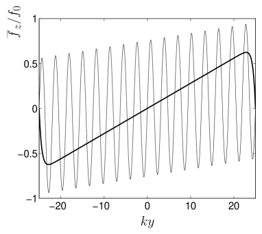
Figure 1: Out-of plane spin polarization induced by an electric field applied parallel to the stripe of a 2DHG (with $\gamma=0.5$). The thick and thin lines were calculated with $\Omega=0.25$ and $\Omega=0.5$, respectively.

An interesting effect, which we do not follow up in this paper, results from the $y$ dependence of the charge density $\overline{f}$ that is strongly affected by the boundary condition and that gives rise to a self-consistent electric field oriented along the $y$ direction. In Fig. 1, the thick line illustrates the result for the spin polarization in the diffusive regime ($D_{z}>0$), when the spin-orbit coupling is weak $\Omega<1/\sqrt{12}$. The electric field aligned along the $x$ axis induces a spin polarization at the edges of the stripe. This SHE has received a great deal of attention. Most popular is the description by means of a spin current oriented perpendicular to the electric field. Many theoretical studies (see, for instance, Ref.[PRB_085308, ; PRB_193316, ]) introduced the spin current $\widehat{J}_{\mu}^{i}$ by a symmetrized product of spin and velocity operators $(\widehat{v}_{\mu}\sigma^{i}+\sigma^{i}\widehat{v}_{\mu})/2$. It was claimed that at least for the cubic Rashba model, the SHE introduced in such a manner is robust against disorder. Experimental results PRL_047204 seem to confirm this physical picture. However, there is a principal difficulty with such an approach. The above mention definition of the current is not sufficiently general. It would completely fail for any hopping transport problem, for which the eigenstates have no dispersion. This definition only applies, whenever the Hamiltonian commutes with the dipole operator. Obviously, this is not the case for the Rashba Hamiltonian. Consequently, it is necessary to go back to the more general definition, which expresses the current by the time derivative of the dipole operator. PRL_076604 ; PRB_165313 This more general treatment of the spin current reveals a close relationship between the field-induced spin accumulation and the spin current expressed by a quasi-chemical potential. From a technical point of view, the current that applies in its most general form to a homogeneous system is calculated from the quantity $\nabla_{\bm{\kappa}}\widehat{f}({\bm{k}},{\bm{\kappa}})$ at ${\bm{\kappa}}={\bm{0}}$ and not only from the density matrix $\widehat{f}({\bm{k}})$. Based on this general definition of the spin current, it was concluded that an electric-field-induced steady-state spin-Hall current does not exist in the cubic Rashba model. JPCM_7497 On the other hand, a SHE was demonstrated by a recent experiment. PRL_047204 This calamity indicates that the notion of a spin current is not useful for studying the SHE. An alternative, which is proposed in this paper, determines the spin accumulation from quantum kinetic equations or the associated spin-charge coupled drift-diffusion equations. The specific difficulty of the latter approach is the formulation of appropriate boundary conditions. PRB_113309 ; PRB_115331

The character of the SHE dramatically changes in strongly spin-orbit coupled systems ($\Omega>1/\sqrt{12}$ so that $D_{z}<0$). The result is illustrated in Fig. 1 by the thin line. A spin-coherent standing wave travels through the stripe. It is remarkable that these oscillations are not damped although a finite elastic scattering is present. The occurrence of a periodic spin pattern is not unusual and has been investigated in the literature. PRB_155317 ; PRB_033316 ; PRB_195308 ; PRB_205307 The novelty here is that such an oscillatory spin pattern can be induced by an electric field. The rapid variation of the out-of plane spin polarization induces a magnetic field that leads to circulating microscopic currents. The retroaction of these currents on spin may result in a finite damping of spin oscillations.

In the strong-coupling limit ($\Omega=K(k)l\gg 1$), the oscillatory spin pattern changes on a length scale $K^{-1}(k)$ that is much smaller than the mean-free path $l$. This fact conflicts with basic assumptions of the drift-diffusion approach, which is only applicable for diffusion lengths much smaller than the mean-free path. Although macroscopic transport equations were found to be valid even when the spin-diffusion length is somewhat less than the mean-free path PRB_212410 , it is indispensable to treat this point in detail. Large values for $\Omega$ give rise to spin-relaxation times $\tau_{sz}$, which are much smaller than the elastic scattering time $\tau$. This condition characterizes the ballistic spin regime. Therefore, we go back to the kinetic Eqs. (3) and (4) and solve them under the condition $\tau\rightarrow\infty$ and to first order in the electric field. For the out-of plane spin polarization, we obtain

$$(\sigma^{2}+4\omega_{k}^{2})f_{z}+\frac{eE\sigma}{\hbar}\frac{\partial}{\partial k_{x}}f_{z}=\frac{2i}{\sigma}({\bm{\omega}}_{{\bm{k}}x}{\bm{\omega}}_{{\bm{\kappa}}y}-{\bm{\omega}}_{{\bm{k}}y}{\bm{\omega}}_{{\bm{\kappa}}x})f_{0},$$ (13)

where $\sigma=s-i{\bm{\kappa}}\cdot{\bm{v}}$. Calculating the inverse Laplace and Fourier transformation and integrating over the angle $\varphi$, we arrive at the analytical solution

$$f_{z}(k,{\bm{r}},t)=\frac{3f_{0}}{16\pi r}\frac{\partial}{\partial k}\left[\frac{eE}{\varepsilon_{k}}\left(\frac{\sin 2K(k)r}{2K(k)r}-\cos 2K(k)r\right)\right]$$

$$\times\left\{\begin{array}[]{ccc}\delta(y-\sqrt{(vt)^{2}-x^{2}})&{\rm for}&0<y\leq vt\\ -\delta(y+\sqrt{(vt)^{2}-x^{2}})&{\rm for}&vt\leq y<0\\ \end{array}\right.\,,$$ (16)

which describes the field-induced spin polarization that occurs, when initially a drop of charge carriers is injected into the 2DHG at the position ${\bm{r}}={\bm{0}}$.

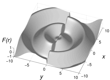
Figure 2: The amplitude $F(r)=\eta x{\rm d}((\sin x/x-\cos x)/x)/{\rm d}x$ in dependence on $r$ with $x=2K(k_{F})r$ and $K(k_{F})=0.5$. For the factor $\eta$, we have: $\eta=\pm 1$ for $y\gtrless 0$.

A $\delta$-like wave front of spin polarization travels through the homogeneous 2DHG. The amplitude of this narrow wave front oscillates as illustrated in Fig. 2. As expected, the relief is antisymmetric with respect to the $y$ axis. Most interesting for our comparison with the above drift-diffusion approach is the observation that the wavelength of the spatial spin pattern is of the order of $K^{-1}(k_{F})$. Therefore, this exact analytical result confirms the existence of a field-induced long-living spin pattern in strongly spin-orbit coupled systems as predicted by the drift-diffusion equations.

Our study of electric-field induced spin phenomena revealed a close relationship between the SHE and spin-coherent oscillations. We compare this conclusion with recent results that demonstrated that the intrinsic SHE and the zitterbewegung are essentially the same kind of phenomena. PRB_205307 Consequently, the question arises whether the above treated spin-coherent waves have to be identified with the zitterbewegung, which is a purely relativistic effect. Indeed, both kinds of oscillatory spin excitations exhibit common features. The characteristic wavelength of both types of oscillations amounts about $100$ nm (calculated by adopting the typical values $\alpha m/\hbar^{2}\sim 2$ nm and $k_{F}\sim 0.1$ nm). Moreover, both the zitterbewegung PRL_206801 and the spin-coherent waves [cf. Eq. (12)] are resonantly enhanced, whenever the width of the stripe matches a characteristic wavelength of the spin excitation. However, some features of spin-coherent waves are not compatible with such an identification with the zitterbewegung. The dispersion relation of coupled spin-charge excitations is calculated from the vanishing determinant of Eqs. (7) and (8). In general, one obtains not only spin-coherent solutions but also damped excitations, whereas the transition between them could be driven by the electric field. In addition, the spin-coherent waves that appear at strong spin-orbit coupling are separated from the SHE by a sharp threshold. For the zitterbewegung such a threshold is not expected as its existence is solely due to at least two energy bands separated by a nonzero gap. We think that the interesting study of the relationship between spin-coherent waves, the zitterbewegung, and long-living spin-coherent states PRB_155317 will continue in the near future.

The experimental observation of the field-induced spin-coherent waves should be possible by high-resolution scanning-probe microscopy imaging techniques. The direct experimental proof of this effect would fascilitate developments both in spintronics and basic research.

This work was supported by the Deutsche Forschungsgemeinschaft and the Russian Foundation of Basic Research under the grant number 05-02-04004.

References

- (1) S. Murakami, N. Nagaosa, and S. C. Zhang, Science 301, 1348 (2003).
- (2) J. Sinova, D. Culcer, Q. Niu, N. A. Sinitsyn, T. Jungwirth, and A. H. MacDonald, Phys. Rev. Lett. 92, 126603 (2004).
- (3) Y. K. Kato, R. C. Myers, A. C. Gossard, and D. D. Awschalom, Science 306, 1910 (2004).
- (4) V. Sih, W. H. Lau, R. C. Myers, V. R. Horowitz, A. C. Gossard, and D. D. Awschalom, Phys. Rev. Lett. 97, 096605 (2006).
- (5) J. Wunderlich, B. Kaestner, J. Sinova, and T. Jungwirth, Phys. Rev. Lett. 94, 047204 (2005).
- (6) J. Shi, P. Zhang, D. Xiao, and Q. Niu, Phys. Rev. Lett. 96, 076604 (2006).
- (7) V. V. Bryksin and P. Kleinert, Phys. Rev. B 73, 165313 (2006).
- (8) O. Bleibaum and S. Wachsmut, Phys. Rev. B 74, 195330 (2006).
- (9) T. L. Hughes, Y. B. Bazaliy, and B. A. Bernevig, Phys. Rev. B 74, 193316 (2006).
- (10) J. Schliemann and D. Loss, Phys. Rev. B 71, 085308 (2005).
- (11) P. Kleinert and V. V. Bryksin, J. Phys.: Condens. Matter 18, 7497 (2006).
- (12) O. Bleibaum, Phys. Rev. B 74, 113309 (2006).
- (13) V. M. Galitski, A. A. Burkov, and S. D. Sarma, Phys. Rev. B 74, 115331 (2006).
- (14) Y. V. Pershin, Phys. Rev. B 71, 155317 (2005).
- (15) J. Wang, K. S. Chan, and D. Y. Xing, Phys. Rev. B 73, 033316 (2006).
- (16) Y. Jiang, Phys. Rev. B 74, 195308 (2006).
- (17) P. Brusheim and H. Q. Xu, Phys. Rev. B 74, 205307 (2006).
- (18) D. R. Penn and M. D. Stiles, Phys. Rev. B 72, 212410 (2005).
- (19) J. Schliemann, D. Loss, and R. M. Westervelt, Phys. Rev. Lett. 94, 206801 (2005).