Surface imaging of inelastic Friedel oscillations

Abstract

Impurities that are present on the surface of a metal often have internal degrees of freedom. Inelastic scattering due to impurities can be revealed by observing local features seen in the tunneling current with scanning tunneling microscope (STM). We consider localized vibrational modes coupled to the electronic structure of a surface. We argue that vibrational modes of impurities produce Fermi momentum $k_{F}$ oscillations in second derivative of current with respect to voltage $\partial^{2}I({\bf r},V)/\partial V^{2}$. These oscillations are similar to the well known Friedel oscillations of screening charge on the surface. We propose to measure inelastic scattering generated by the presence of the vibrational modes with STM by imaging the $\partial^{2}I/\partial V^{2}$ oscillations on the metal surface.

I Introduction

Inelastic electron tunneling spectroscopy (IETS) with scanning tunneling microscope, IETS-STM, is a well-established technique, starting with an important experiment by Stipe et al.stipe1998 These experiments show step like features in the tunneling current and local density of states (DOS). The physical explanation of the effect is straightforward: once the energy of the tunneling electron exceeds the energy required to excite local vibrations, there is a new scattering process that contributes to the scattering of electrons due to inelastic excitation of the local mode.jaklevich1966 The local vibrational modes can be seen in differential conductance measurements as side-bands to the main (elastic) conductance peak.park2000 Recently, IETS-STM was used to measure the spin excitations of individual magnetic atoms.heinrich2004 In addition, recent experiments show dominant inelastic channels which are strongly spatially localized to particular regions of a molecule.grobis2005

Improvements in spectroscopic and microscopic measurements have provided new information about fundamental aspects of scattering and interactions in the solid state. Recently, STM technique has evolved from imaging of surfaces,binnig1987 to spin polarized tips for magnetic sensitivity of the read-outheinrich2004 and spin-polarized injection of the tunneling current used in the measurements.wiesendanger STM has been also used to detect Kondo interactions between conduction electrons and single atomic spinsmadhavan1998 ; li1998 and to study the properties of individual atoms.yamasaki2003 ; bode2004

We propose to use resolution of STM to address spatially resolved inelastic tunneling features produced by local inelastic scattering of the molecule both near the scattering center and at far distances. The ”fingerprint” of the inelastic scattering will be present even away from the scattering center. Using local IETS-STM would enable measurements of the standing waves produced by inelastic scattering off impurities, which could be revealed as waves seen in the second derivative $\partial^{2}I({\bf r},V)/\partial V^{2}$. For the simplest model of parabolic conduction band these waves will be seen as standing waves with period set by the Fermi momentum $k_{F}$. These standing waves are seen in the oscillations of the $\partial^{2}I({\bf r},V)/\partial V^{2}$ and are similar but qualitatively different from the conventional Friedel oscillations.

In case of regular Friedel oscillations the charge that screens off the impurity exhibit oscillations at large distances from the impurity. Recent STM measurements have observed Friedel oscillations in the elastic scattering channels on surfaces with atomic impurities adsorbed on the surface.madhavan1998 ; morgenstern2004 These oscillations are seen in a wide range of bias as they reflect screening of the charge by electron states in the whole bandwidth. Inelastic scattering of surface electrons off the molecules may be viewed as inelastic Friedel oscillations produced by the electron states that are involved in screening. Inelastic Friedel oscillations are seen only in the narrow window of energies near the energy of the mode $\omega_{0}$ at which inelastic scattering occurs, in contrast to conventional Friedel screening.

It was recently proposed to use IETS-STM to address the inelastic scattering features in the Bi2212 superconductors.zhu2006 ; balatskyRMP2006 In the case of superconductors, the situation is more involved since one has to deal with the more complicated band structure of Bi2212 and with the inelastic scattering off the distributed bosonic modes. The work presented here allows one to test similar ideas in a more controlled set up where the metal surface and molecular modes are well understood.

The paper is organized as follows. In Sec. II we introduce a model which describe the addressed issue and some numerical results are discussed in Sec. III. The paper is concluded in Sec. IV.

II Probing the Friedel oscillations and inelastic scattering measurements

The system we consider consists of a two-dimensional surface on which inelastic scattering centers are randomly distributed. For simplicity, we assume that the impurities are distributed sufficiently far from each other so that their mutual interactions can be neglected. All vibrational modes have energy $\omega_{0}$ and are assumed to be the same as they would come from the same type of molecules. We use the Hamiltonian for the local vibrational modes, coupled to electrons via Holstein coupling with interactions assumed to occur only at the single impurity site, so that

$${\cal H}=\sum_{{\bf k}\sigma}\varepsilon_{{\bf k}}c_{{\bf k}\sigma}^{\dagger}c_{{\bf k}\sigma}+\omega_{0}b^{\dagger}b+\lambda\sum_{{\bf k}{\bf k}^{\prime}\sigma}c_{{\bf k}\sigma}^{\dagger}c_{{\bf k}^{\prime}\sigma}(b^{\dagger}+b).$$ (1)

Here, a surface electron is created (annihilated) by $c_{{\bf k}\sigma}^{\dagger}\ (c_{{\bf k}\sigma})$ at the energy $\varepsilon_{{\bf k}}$. The strength of the electron-phonon interaction is given by the parameter $\lambda$, whereas $\omega_{0}$ is the mode of the bare phonon which is created (annihilated) by $b^{\dagger}\ (b)$.

The features we are considering should be seen in the second derivative of the tunneling current with respect to the bias voltage $V$ in real space, i.e. $\partial^{2}I({\bf r},V)/\partial V^{2}$. This quantity is directly proportional to the frequency derivative of the local DOS. In second order perturbation theory, this amounts to taking the frequency derivative of the correction to the density of states, $\delta N({\bf r},\omega)$, due to the influence of the impurity scattering. The real space electron Green function (GF) is given by

$$G({\bf r},{\bf r}^{\prime};\omega)=G_{0}({\bf r},{\bf r}^{\prime};\omega)+G_{0}({\bf r},0;\omega)\Sigma(\omega)G_{0}(0,{\bf r}^{\prime};\omega),$$ (2)

with the zero GF in two spatial dimensions

$$G_{0}({\bf r},{\bf r}^{\prime};\omega)=\sum_{\bf k}G_{0}({\bf k};\omega)e^{i{\bf k}\cdot({\bf r}-{\bf r}^{\prime})}$$ (3)

$$= 2\pi\frac{m}{\hbar^{2}}J_{0}(k_{F}|{\bf r}-{\bf r}^{\prime}|)\biggl{(}\log\biggl{|}\frac{\omega+D}{\omega-D}\biggr{|}-i\pi\biggr{)}.$$

Here, the bare electron Fourier transformed GF $G_{0}({\bf k},\omega)=1/(i\omega-\varepsilon_{{\bf k}})$. Using standard procedure for frequency summation, the self-energy $\Sigma(\omega)$ is found as

$$\Sigma(i\omega)=-\frac{\lambda^{2}}{\beta}\sum_{{\bf k},m}G_{0}({\bf k},i\omega+i\Omega_{m})D_{0}(i\Omega_{m})$$

$$= \lambda^{2}\sum_{\bf k}\biggl{\{}\frac{n_{B}(\omega_{0})+f(\varepsilon_{{\bf k}})}{i\omega+\omega_{0}-\varepsilon_{{\bf k}}}+\frac{n_{B}(\omega_{0})+1-f(\varepsilon_{{\bf k}})}{i\omega-\omega_{0}-\varepsilon_{{\bf k}}}\biggr{\}},$$

where $D_{0}(i\omega)=2\omega_{0}/(\omega^{2}-\omega_{0}^{2})$ is the bare phonon GFs.

Due to these definitions, it is clear that the correction to the local DOS is given by

$$\delta N({\bf r},\omega)=\frac{1}{\pi}{\rm Im}G_{0}({\bf r},0,\omega)\Sigma(\omega)G_{0}(0,{\bf r},\omega)$$ (5)

Since the effects from inelastic scattering are included in the self-energy, we evaluate $\partial\delta N(\omega)/\partial\omega$, which is directly proportional to $\partial^{2}I({\bf r},V)/\partial V^{2}$.

Sharp feature in self-energy ${\rm Im}\Sigma(\omega)$ is connected to the inelastic scattering feature. Noting that ${\rm Re}G_{0}({\bf r},{\bf r}^{\prime},\omega)\approx 0$, our calculations simplify to $\delta N({\bf r},\omega)\approx(1/\pi)G_{0}({\bf r},0;\omega)[{\rm Im}\Sigma(\omega)]G_{0}(0,{\bf r};\omega)$. We thus find that

$$\delta N({\bf r},\omega)\approx-\pi^{3}\biggl{(}\frac{2m}{\hbar^{2}}\biggr{)}^{2}J_{0}^{2}(k_{F}r){\rm Im}\Sigma(\omega).$$ (6)

Analytical continuation, e.g. $i\omega\rightarrow\omega+i0^{+}$, of the self-energy in Eq. (II) gives the imaginary part

$${\rm Im}\Sigma(\omega) = -2\pi^{2}\lambda^{2}\frac{m}{\hbar^{2}}[2n_{B}(\omega_{0})+1$$ (7)

$$+f(\omega+\omega_{0})-f(\omega-\omega_{0})].$$

The correction to the local DOS provides the oscillation in real space. The electron-phonon interaction gives rise to an increased local DOS for frequencies $|\omega|>\omega_{0}$.

We find that $\partial^{2}I({\bf r},V)/\partial V^{2}$ is proportional to

$$\frac{\partial}{\partial\omega}\delta N({\bf r},\omega)\approx-\pi^{3}\biggl{(}\frac{2m}{\hbar^{2}}\biggr{)}^{2}J_{0}^{2}(k_{F}r)\frac{\partial}{\partial\omega}{\rm Im}\Sigma(\omega),$$ (8)

where

$$\frac{\partial}{\partial\omega}{\rm Im}\Sigma(\omega)=2\pi^{2}\lambda^{2}\frac{m}{\hbar}\frac{\beta}{4}\biggl{(}\cosh^{-2}\frac{\beta}{2}(\omega+\omega_{0})$$

$$-\cosh^{-2}\frac{\beta}{2}(\omega-\omega_{0})\biggr{)}.$$ (9)

taking $(\beta/4)\cos^{-2}\beta(\omega\pm\omega_{0})/2\rightarrow\delta(\omega\pm\omega_{0})$, as $T\rightarrow 0$, we expect to find sharp features in $\partial^{2}I({\bf r},V)/\partial V^{2}$ around $\omega=\pm\omega_{0}$ for low temperatures. Hence, our simplified analytical calculations show that inelastic impurities that couple to the surface electrons give rise to Friedel oscillations in the real space image of $\partial^{2}I({\bf r},V)/\partial V^{2}$.

One important point that we also need to address is the role of the dephasing in the inelastic scattering process. We are dealing with the inelastic scattering process in which the incoming and outgoing electron waves have different energy. Energy transferred to/from the inelastic center implies the phase change and hence the interference of the incoming and outgoing waves will be affected by dephasing caused by scattering. This dephasing process would occur even at $T=0$ and hence has nothing to do with the thermal scattering. In the limit of small boson energy $\hbar\omega_{0}\ll E_{F}$ dephasing is small and is not going to destroy the interference of the incoming and outgoing waves. Qualitatively we can estimate the change in the phase as a result of inelastic scattering as $\delta\phi=\delta\epsilon\delta t$. Here $\delta\epsilon=\hbar\omega_{0}$ is the energy transferred to/from the electron and $\delta t\sim a/v_{F}$ is the typical time for the collision of electron with the impurity of size $a$, assumed to be on the unit cell size. Then we estimate $a=2\pi/k_{F}$ and obtain

$$\delta\phi\sim 2\pi\hbar\omega_{0}/E_{F}\ll 2\pi.$$ (10)

Therefore the interference between incoming and outgoing waves will survive as long as energy transferred in the collision is small.

III Results

Although the analytical calculations in Sec. II clearly shows oscillatory response of the inelastic scattering, we provide in this section some numerical results to emphasize our proposal. The numerical calculations of $\delta N({\bf r},\omega)$ are based on the full expression presented in Appendix A.

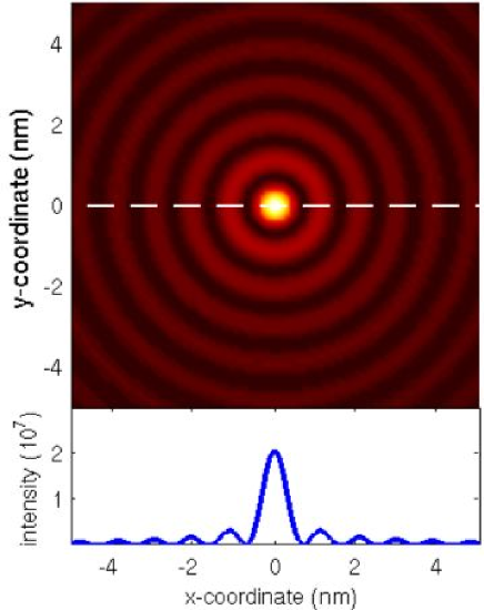
Figure 1: (Color online) Spatial dependence of $\delta N({\bf r}-{\bf r}_{0},\omega=\omega_{0})$, for $T=1$ K.

From Eq. (8) it is clear that the oscillations only have a radial component, because the assumed electron-phonon coupling is rotationally invariant. This feature is manifested in Fig. 1, where the upper panel shows the spatial dependence of $\delta N({\bf r}-{\bf r}_{0},\omega_{0})$ at the resonance energy $\omega=\omega_{0}$. The lower panel shows the intensity of $\delta N(x-x_{0},0;\omega_{0})$, on the line ${\bf r}-{\bf r}_{0}=x-x_{0}$, which corresponds to the dashed line in the upper panel. The features in $\delta N({\bf r}-{\bf r}_{0},\omega)$ depend on the spatial position and on the frequency. In Fig. 2, which shows a contour plot of $\delta N(x-x_{0},0;\omega)$, we illustrate the fact that the inelastic Friedel oscillations occur in a narrow interval around $\omega=\pm\omega_{0}$. The plot clearly illustrates that there is hardly any intensity at all, for frequencies off the phonon mode $\omega_{0}$.

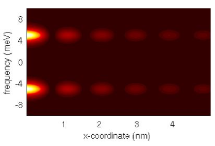
Figure 2: Spatial and frequency dependence of $|\partial\delta N({\bf r},\omega)/\partial\omega|$ at $T=5$ K.

The plot in Fig. 3 illustrates the IETS-STM resonance signal on a surface with four inelastic scattering centers, analogous to the plot in Fig. 1. As expected from the wave character of the signal, the pattern on the surface is because of interfering Friedel oscillations from the four scattering centers.

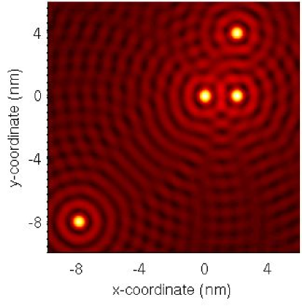
Figure 3: (Color online) Calculated IEST-STM resonance, e.g. at phonon mode resonance, signal on surface with four inelastic impurities embedded.

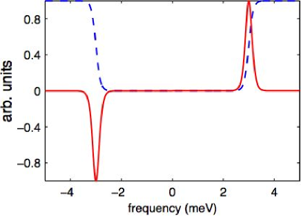
Figure 4: (Color online) $\partial\delta N(0,\omega)/\partial\omega$ (solid) and $\delta N(0,\omega)$ (dashed) for $\omega_{0}=3$ meV and $T=1$ K ($m=\hbar=1$).

Next suppose that the position of the STM tip is kept fixed in space, i.e. letting ${\bf r}-{\bf r}_{0}=0$ where ${\bf r}_{0}$ is the position of the inelastic scattering center. Then, as show in the previous section, the derivative $\partial\delta N(0,\omega)/\partial\omega$ is expected to peak or dip at $\omega=\pm\omega_{0}$, c.f. Eq. (8) and (9), as the frequency is varied. This is illustrated in Fig. 4 (solid). These local extrema correspond to steps in $\delta N(0,\omega)$, which is also clear in Fig. 4 (dashed).

From Eq. (9) we find that intensity of the peaks in $|\partial\delta N/\partial\omega|$ is highly temperature dependent, which is illustrated in Fig. 5 for two temperatures. The plots clearly shows that the peaks are becomes sharper for decreasing temperatures, illustrating the $\delta$ function like behavior at low temperatures.

IV Conclusions

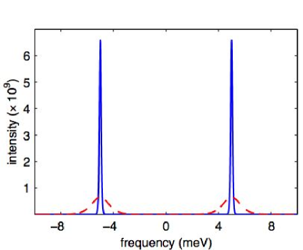
Figure 5: (Color online) The derivative ($|\partial\delta N/\partial\omega|$) for different temperatures $T\in\{0.01,0.1\}$ K $\{$solid, dashed$\}$. The plots have been artificially broadened.

We propose a scanning technique that allows one to visualize the oscillations in the inelastic scattering produced by the local modes. Standard way to image IETS of the molecule is to measure $\partial^{2}I({\bf r},V)/\partial V^{2}$ locally near the scattering center.stipe1998 ; heinrich2004 ; grobis2005 We point out that the ”fingerprint” of the inelastic scattering will be present even away from the scattering center. The incoming electron wave donates/absorbs energy from the inelastic scattering center. In the process of inelastic scattering the incoming and outgoing electron waves interfere. This interference will can be clearly seen in the real space oscillations of the second derivative $\partial^{2}I({\bf r},V)/\partial V^{2}$ with characteristic momentum $k_{F}$. The important point is that for the flat density of states the interference between states that undergone inelastic scattering will only be present at the bias $eV=\hbar\omega_{0}$ and not at other energies. This makes the proposed effect very different from the conventional Friedel oscillations that occur for elastic scattering and are present for the wide range of energies as the whole band of electrons participates in screening. We also argue that as long as the energy difference between these states is small compared with the Fermi energy of electrons, the dephasing in the process of scattering is small and hence interference is preserved.

The technique, proposed here, can be applied to the inelastic scattering of the electrons from the local vibrational modes of the molecules on the surface grobis2005 and would offer exciting possibilities to image the interference and interactions between inelastic scattering processes in the ensemble of few scattering centers. In practice the tunneling conductance in real materials will likely have peaks in $\partial^{2}I({\bf r},V)/\partial V^{2}$ as a function of position due to band structure. One would need to be able to separate these peaks from the peaks that arise due to inelastic scattering.

This work has been supported by US DOE, LDRD and BES, and was carried out under the auspices of the NNSA of the US DOE at LANL under Contract No. DE-AC52-06NA25396. We are grateful to M. Crommie, J.C. Davis, D. Eigler, W. Harrison, H. Manoharan, and R. Wiesendanger for useful discussions.

Appendix A Derivation of $\delta N$

In the above analysis we neglected the real part of the unperturbed Green’s functions. However, as we show here, taking this part into account does not significantly change the picture. We have

$$\delta N({\bf r},\omega) = -\frac{1}{\pi}\biggl{(}\frac{2\pi m}{\hbar^{2}}\biggr{)}^{2}J_{0}^{2}(k_{F}r)\biggl{\{}\pi^{2}{\rm Im}\Sigma(\omega)-\biggl{[}{\rm Im}\Sigma(\omega)\log\left|\frac{\omega+D}{\omega-D}\right|-2\pi{\rm Re}\Sigma(\omega)\biggr{]}\log\left|\frac{\omega+D}{\omega-D}\right|\biggr{\}}.$$

Since we are interested in the frequency derivative of this expression we find that

$$\frac{\partial}{\partial\omega}\delta N({\bf r},\omega) = -\frac{1}{\pi}\biggl{(}\frac{2\pi m}{\hbar^{2}}\biggr{)}^{2}J_{0}^{2}(k_{F}r)\biggl{\{}\pi^{2}\frac{\partial}{\partial\omega}{\rm Im}\Sigma(\omega)-\biggl{(}\frac{\partial}{\partial\omega}{\rm Im}\Sigma(\omega)\biggr{)}\log\left|\frac{\omega+D}{\omega-D}\right|$$

$$+{\rm Im}\Sigma(\omega)\frac{4D}{\omega^{2}-D^{2}}\log\left|\frac{\omega+D}{\omega-D}\right|+2\pi\biggl{(}\frac{\partial}{\partial\omega}{\rm Re}\Sigma(\omega)\biggr{)}\log\left|\frac{\omega+D}{\omega-D}\right|-2\pi{\rm Re}\Sigma(\omega)\frac{2D}{\omega^{2}-D^{2}}\biggr{\}}$$

Here,

$${\rm Re}\Sigma(\omega) = 2\pi\lambda^{2}\frac{m}{\hbar^{2}}\int\biggl{\{}\frac{n_{B}(\omega_{0})+f(\varepsilon)}{\omega+\omega_{0}-\varepsilon}+\frac{n_{B}(\omega_{0})+1-f(\varepsilon)}{\omega-\omega_{0}-\varepsilon}\biggr{\}}d\varepsilon$$

$$= 2\pi\lambda^{2}\frac{m}{\hbar^{2}}\biggl{\{}n_{B}(\omega_{0})\log\left|\frac{\omega+\omega_{0}+D}{\omega+\omega_{0}-D}\right|+[n_{B}(\omega_{0})+1]\log\left|\frac{\omega-\omega_{0}+D}{\omega-\omega_{0}-D}\right|-2\omega_{0}\int\frac{f(\varepsilon)}{(\omega-\varepsilon)^{2}-\omega_{0}^{2}}d\varepsilon\biggr{\}}$$

which gives the derivative

$$\frac{\partial}{\partial\omega}{\rm Re}\Sigma(\omega) = -2\pi\lambda^{2}\frac{m}{\hbar^{2}}\int\biggl{\{}\frac{n_{B}(\omega_{0})+f(\varepsilon)}{(\omega+\omega_{0}-\varepsilon)^{2}}+\frac{n_{B}(\omega_{0})+1-f(\varepsilon)}{(\omega-\omega_{0}-\varepsilon)^{2}}\biggr{\}}d\varepsilon$$

$$= 4\pi\lambda^{2}\frac{m}{\hbar^{2}}\biggl{\{}D\frac{n_{B}(\omega)}{(\omega+\omega_{0})^{2}-D^{2}}+D\frac{n_{B}(\omega_{0})+1}{(\omega-\omega_{0})^{2}-D^{2}}+2\omega_{0}\int f(\varepsilon)\frac{\omega-\varepsilon}{[(\omega-\varepsilon)^{2}-\omega_{0}^{2}]^{2}}d\varepsilon\biggr{\}}$$

However, since the logarithm $\log|(\omega\pm\omega_{0}+D)/(\omega\pm\omega_{0}-D)|\approx 0$ for $D\gg|\omega\pm\omega_{0}|$ we see that all terms but the first are negligible in $\partial\delta N/\partial\omega$.

References

• (1) B. C. Stipe, M. A. Rezaei, and W. Ho, Science, 280, 1732 (1998).
• (2) R. C. Jaklevich and J. Lambe, Phys. Rev. Lett. 17, 1139 (1966); J. Lambe and R. C. Jaklevich, Phys. Rev. 165, 821 (1968).
• (3) H. Park, J. Park, A. K. L. Lim, E. H. Anderson, A. P. Alivisatos, and P. L. McEuen, Nature, 407, 57 (2000).
• (4) A. J. Heinrich, J. A. Gupta, C. P. Lutz, and D. M. Eigler, Science, 306, 466 (2004); C. F. Hirjibehedin, C. P. Lutz, and A. J. Heinrich, Science, 312, 1021 (2006).
• (5) M. Grobis, K. H. Khoo, R. Yamachika, X. Lu, K. Nagaoka, S. G. Louie, M. F. Crommie, H. Kato, and H. Shinohara, Phys. Rev. Lett. 94, 136802 (2005).
• (6) G. Binnig and H. Rohrer, Rev. Mod. Phys. 59, 615 (1987).
• (7) S. Heinze et al., Science 288, 1805 (2000); A. Kubetzka , M. Bode, O. Pietzsch, and R. Wiesendanger, Phys. Rev. Lett. 88, 057201 (2002); A. Wachowiak et al., Science 298, 577 (2002); J. Wiebe et al., Rev. Scientific Instruments, 75, 4871 (2004).
• (8) V. Madhavan, W. Chen, T. Jamneala, M. F. Crommie, and N. S. Wingreen, Science, 280, 567 (1998); Phys. Rev. B, 64, 165412 (2001).
• (9) J. Li, W. -D. Schneider, R. Berndt, and B. Delley, Phys. Rev. Lett. 80, 2893 (1998).
• (10) A. Yamasaki, W. Wulfhekel, R. Hertel, S. Suga, and J. Kirschner, Phys. Rev. Lett. 91, 127201 (2003).
• (11) M. Bode, O. Pietzsch, A. Kubetzka, and R. Wiesendanger, Phys. Rev. Lett. 92, 067201 (2004).
• (12) K. Morgenstern, K. -F. Braun, and K. -H. Rieder, Phys. Rev. Lett, 93, 056102 (2004).
• (13) J. -X. Zhu, A. V. Balatsky, T. P. Devereaux, Q. Si, J. Lee, K. McElroy, and J. C. Davis, Phys. Rev. B, 73, 014511 (2006).
• (14) A. V. Balatsky, I. Vekhter, and J. -X. Zhu, Rev. Mod. Phys. 78, 373 (2006).