Dynamical mean field theory of the Gutzwiller-projected BCS Hamiltonian: Phase fluctuations and the pseudogap

Abstract

One of the most prominent problems in high temperature superconductivity is the nature of the pseudogap phase in underdoped regimes; particularly important is the role of phase fluctuations. The Gutzwiller-projected BCS Hamiltonian is a useful model for high temperature superconductivity due to an exact mapping to the Heisenberg model at half filling and generally a very close connection to the $t$-$J$ model at moderate doping. We develop the dynamical mean field theory for the $d$-wave BCS Hamiltonian with on-site repulsive interaction, $U$, physically imposing the partial Gutzwiller projection. For results, two pseudogap energy scales are identified: one associated with the bare pairing gap for the singlet formation and the other with the local phase coherence. The real superconducting gap determined from sharp coherence peaks in the density of states shows strong renormalization from the bare value due to $U$.

I Introduction

Among the most fundamental issues in high temperature superconductivity is the pairing mechanism. However, even without its specific knowledge, many properties of the superconducting phase can be well understood in the framework of the conventional BCS theory with modification of the $d$-wave pairing symmetry. On the other hand, there are a variety of peculiar behaviors observed in cuprates, which cannot be explained within the conventional BCS theory. These unconventional behaviors are pronounced in underdoped regimes where superconducting order is subject to strong phase fluctuations. While experimental setups are diverse, these unconventional behaviors can be attributed to the existence of an energy gap called the pseudogap LeeNagaosaWen ; Timusk . Complete understanding of high temperature superconductivity, therefore, requires a consistent theoretical framework which not only provides an explanation for pairing, but also contains the pseudogap phenomenon as a natural part.

Experiments in fact suggest two distinctive pseudogaps LeeNagaosaWen . In the first class of experiments, the pseudogap phenomenon can be understood in terms of the formation of spin singlet pairs. Since spin singlet states are rigid against spin flip, it is expected that, if there remains a tendency toward the singlet formation even above $T_{c}$, the spin susceptibility should be reduced from that of the paramagnetic phase, which is indeed consistent with Knight-shift measurements Curro . Also, the decrease in the specific heat Loram can be understood in terms of the spin entropy loss. Furthermore, the high temperature pullback of the leading edge observed in angle-resolved photoemission spectroscopy ARPES can be interpreted as a consequence of the energy cost in breaking pairs. The gap formation in the frequency-dependent $c$-axis conductivity caxis can be also explained similarly.

In the second class of experiments, the pseudogap phenomenon is understood so that, despite the absence of global coherence, the local phase is well defined. The main experimental tool in this class is the Nernst-effect measurement where a large Nernst signal indicates the presence of well-defined vortices and therefore a phase coherence at least in a local scale Nernst . The importance of superconducting phase fluctuations at low doping was first noted by Emery and Kivelson EmeryKivelson , who conjectured that the whole pseudogap regime might be explained by a robust pairing amplitude in the presence of strong phase fluctuations. The problem, however, is that the pairing amplitude itself is not robust when phase fluctuations are very strong. Since the electron number is conjugate with the phase, small fluctuations in electron number at low doping give rise to large fluctuations in phase. So, while the pseudogap associated with the singlet formation remains finite even at low doping, the one associated with the local phase coherence vanishes, as seen experimentally.

Therefore, it is important to distinguish the above two pseudogap phenomena: one associated with the singlet formation and the other with the local phase coherence. On the other hand, the real superconducting gap is determined from the formation of sharp coherence peaks in the density of states. In technical terms, the real superconducting gap is identified with the fully renormalized pairing amplitude while the pseudogap associated with the singlet formation is the bare pairing amplitude. From this view, the pseudogap associated with local phase coherence is a crossover energy scale for a partial coherence. In this paper, we would like to provide a theoretical framework which addresses these issues in a computationally reliable manner.

To this end, the rest of the paper is organized as follows. We begin in Section II by providing a physical motivation for the main Hamiltonian of the paper, i.e., the BCS Hamiltonian with on-site repulsive interaction, $U$, which becomes identical to the Gutzwiller-projected BCS Hamiltonian in the large $U$ limit. We call this Hamiltonian the BCS+$U$ Hamiltonian. In Section III the dynamical mean field theory (DMFT) is formulated for the analysis of the BCS+$U$ Hamiltonian in order to study $d$-wave superconducting fluctuations under the influence of $U$. Our DMFT formalism maps the full lattice model to an effective model for an impurity submerged in $d$-wave superconducting media. In Section III.1, we provide an argument for the applicability of the single-site DMFT formalism for the description of superconducting fluctuations near the insulating phase transition. Note that such situation can be obtained, for example, at sufficiently low doping close to the Néel state, which is actually the main region of interest in this work. It is further supported by large-scale exact diagonalization that the assumption of the single-site DMFT formalism can be in fact valid even away from the phase transition point as long as the $d$-wave pairing amplitude is appropriately chosen in the bare level. Detailed derivation of the DMFT self-consistency equations is presented in Section III.2.

Main results are reported in Section IV. First, in Section IV.1, we show that, at half filling, there is a close similarity between the local physics of the Hubbard model and the strongly-paired BCS+$U$ model, which is fundamentally connected to the precise equivalence between the Heisenberg model and the strongly-paired Gutzwiller-projected BCS model Park . We then show in Section IV.2 that the superconductor-to-insulator transition is mainly caused by the collapse of the quasiparticle spectral weight (or the $Z$ factor) which affects both the quasiparticle effective mass and the superconducting amplitude equally. We emphasize our viewpoint that, while the real pairing amplitude is fully renormalized to be zero, the bare pairing amplitude remains non-zero and can be measured in experiments probing local pairing. In Section IV.3 we propose a novel method of computing the local phase stiffness within the DMFT framework. Results from this method explicitly demonstrate that the phase coherence can survive locally even after the global coherence is lost. In Section IV.4 we study the doping dependence of the local density of states (LDOS) which shows that hidden superconductivity reemerges upon doping. The paper is finally concluded in Sec. V where our theory is placed in perspective.

II BCS+$U$ Hamiltonian and the Gutzwiller projection

Our theory is based on the analysis of the Gutzwiller-projected BCS Hamiltonian Park . In particular, we study the $d$-wave BCS Hamiltonian with on-site repulsive interaction, $U$, which plays a role of physically imposing the partial Gutzwiller projection:

$$H_{\textrm{BCS}+U} = -t\sum_{\langle i,j\rangle}(c^{\dagger}_{i\sigma}c_{j\sigma}+\textrm{H.c.})-\mu\sum_{i}c^{\dagger}_{i\sigma}c_{i\sigma}$$ (1)

$$+ \sum_{\langle i,j\rangle}\Delta_{ij}(c^{\dagger}_{i\uparrow}c^{\dagger}_{j\downarrow}-c^{\dagger}_{i\downarrow}c^{\dagger}_{j\uparrow}+\textrm{H.c.})$$

$$+ U\sum_{i}n_{i\uparrow}n_{i\downarrow}\;,$$

where the spin index $\sigma=\uparrow$ or $\downarrow$, $t$ is the hopping amplitude, and $\mu$ is the chemical potential. $\langle i,j\rangle$ indicates that $i$ and $j$ are nearest neighbors. Since we are interested in $d$-wave pairing, the bare pairing amplitude $\Delta_{ij}=\Delta$ for $j=i+\hat{x}$ and $-\Delta$ for $j=i+\hat{y}$. As mentioned previously, we call this model the BCS+$U$ model. The large $U$ limit corresponds to the fully Gutzwiller-projected BCS Hamiltonian.

The main reason for analyzing the Gutzwiller-projected BCS Hamiltonian is the existence of an exact mapping to the Heisenberg model at half filling and generally a very close connection to the $t$-$J$ model at moderate doping, as shown by exact diagonalization as well as analytic treatments Park . We emphasize that, while the Gutzwiller-projected BCS wave function [equivalently the resonating valence bond (RVB) state Anderson ] is not a good wave function at half filling and presumably so at low enough doping, the Gutzwiller-projected BCS Hamiltonian itself serves as a reliable model. Also in a purely phenomenological level the Gutzwiller-projected BCS Hamiltonian can be taken as a good theoretical model since superconductivity in cuprates actually coexists with strong on-site repulsion.

III Formulation of the dynamical mean field theory

For concrete analysis, we develop the dynamical mean field theory (DMFT) for the BCS+$U$ model. In essence, the dynamical mean field theory is a quantum generalization of the classical mean field theory with a key difference that it averages out only spatial variations while fully taking into account quantum-mechanical, temporal fluctuations DMFT_review . For this reason, the dynamical mean field theory is regarded as one of the most powerful theoretical tools in attacking strongly correlated electron problems, provided that spatial fluctuations are not strong enough to significantly modify the bare dispersion. We choose to use the dynamical mean field theory for the analysis of the BCS+$U$ model since it is known that (i) the Fermi surface as well as the gap structure are well described by the bare dispersion of the $d$-wave BCS Hamiltonian, and (ii) the pseudogap also has a similar $d$-wave structure as the real superconducting gap Timusk .

Actually, there have already been previous attempts to use the dynamical mean field theory to investigate the existence of superconductivity in the Hubbard model. The basic idea was to incorporate the superconducting order parameter via the Nambu spinor formalism DMFT_review . A more recent development was to combine the Nambu spinor formalism and the cellular dynamical mean field theory (CDMFT) which enlarges the DMFT impurity from a single site to a cluster KyungTremblay ; Capone . An important advantage of this approach is the flexibility to allow non-local pairing such as $d$-wave since now electrons can be paired with those in other sites within cluster. Our approach is completely different since we first take the Gutzwiller-projected BCS Hamiltonian to be derived from a more fundamental model such as the $t$-$J$ model Park . Knowing that the full Gutzwiller projection is obtained in the large $U$ limit, we then analyze the BCS+$U$ Hamiltonian as a function of $U$ via single-site DMFT techniques. The non-local nature of $d$-wave pairing is embedded in the dispersion of the bare pairing amplitude.

In the following section, we provide an argument that, near the insulating phase transition (for example, at sufficiently low doping), the $d$-wave pairing term present in the bare level is qualitatively sufficient to capture the essence of superconducting fluctuations. It is further supported by exact diagonalization that the assumption of the single-site DMFT formalism is in fact valid even away from the phase transition point as long as the bare $d$-wave pairing amplitude is appropriately chosen.

III.1 Applicability of the single-site DMFT formalism

Let us consider the most general form of the Green’s function:

$$\hat{G}_{\bf k}^{-1}(i\omega) \equiv \left(\begin{array}[]{cc}G_{\bf k}(i\omega)&F_{\bf k}(i\omega)\\ F^{*}_{\bf k}(i\omega)&-G^{*}_{\bf k}(i\omega)\end{array}\right)^{-1}$$ (4)

$$= \left(\begin{array}[]{cc}i\omega-\xi_{\bf k}&\Delta_{\bf k}\\ \Delta_{\bf k}&i\omega+\xi_{\bf k}\end{array}\right)$$ (7)

$$- \left(\begin{array}[]{cc}\Sigma_{\bf k}(i\omega)&S_{\bf k}(i\omega)\\ S^{*}_{\bf k}(i\omega)&-\Sigma^{*}_{\bf k}(i\omega)\end{array}\right)$$ (10)

where $\xi_{\bf k}=\varepsilon_{\bf k}-\mu$. Simple matrix inversion then leads to the following expressions:

$$G_{\bf k}(i\omega)=\frac{-[i\omega+\xi_{\bf k}+\Sigma^{*}_{\bf k}(i\omega)]}{|i\omega-\xi_{\bf k}-\Sigma_{\bf k}(i\omega)|^{2}+|\Delta_{\bf k}-S_{\bf k}(i\omega)|^{2}},$$

$$F_{\bf k}(i\omega)=\frac{\Delta_{\bf k}-S_{\bf k}(i\omega)}{|i\omega-\xi_{\bf k}-\Sigma_{\bf k}(i\omega)|^{2}+|\Delta_{\bf k}-S_{\bf k}(i\omega)|^{2}}.$$ (11)

Now, assuming that the pairing symmetry remains precisely $d$-wave even after $U$, one can generally write that

$$S_{\bf k}(i\omega)=\tilde{S}_{\textrm{odd}}(i\omega)+\tilde{S}_{\textrm{even}}(i\omega)\frac{\Delta_{\bf k}}{\Delta}$$ (12)

where the momentum-independent components, $\tilde{S}_{\textrm{even}}(i\omega)$ and $\tilde{S}_{\textrm{odd}}(i\omega)$, denote even and odd functions of $i\omega$, respectively. Since $\tilde{S}_{\textrm{odd}}(i\omega)$ is a local quantity, it can be computed in the single-site DMFT framework. As presented in Sec. IV, however, our single-site DMFT study shows that $\tilde{S}_{\textrm{odd}}(i\omega)$ is actually zero to within numerical accuracy, eliminating the possibility of odd-frequency pairing. On the other hand, the even-frequency pairing component, $\tilde{S}_{\textrm{even}}(i\omega)$, can be expanded in low energy with even powers of $\omega$: $\tilde{S}_{\textrm{even}}(i\omega)\simeq\tilde{S}_{0}+\tilde{S}_{2}\omega^{2}+\cdots$.

Based on good agreement between the Fermi surface shape obtained from bare hopping parameters (for example, determined in the first-principle calculations) and that of experiment, it can be argued that the leading term of the normal self-energy correction is mostly momentum-independent. In this case, the normal self-energy correction can be computed within the single-site DMFT framework. Explicit numerical computation of our DMFT study shows that $\Sigma(i\omega)\simeq(1-1/Z)i\omega$ in the low-energy limit (Note that the constant term is not explicitly written since it simply shifts the chemical potential and so can be absorbed into $\xi_{\bf k}$). The factor $Z$ is called the quasiparticle spectral weight. After analytic continuation of $i\omega\rightarrow\omega+i\delta$, the pole of the Green’s function is given in the low-energy limit by the following equation:

$$(\omega/Z)^{2}-\xi_{\bf k}^{2}-\Delta_{\bf k}^{2}[1-\tilde{S}_{\textrm{even}}(\omega)/\Delta]^{2}=0\;,$$ (13)

which can be further reduced by expanding $\tilde{S}_{\textrm{even}}(\omega)$ as follows:

$$\left[\frac{1}{Z^{2}}-2\frac{\tilde{S}_{2}}{\Delta}\left(1-\frac{\tilde{S}_{0}}{\Delta}\right)\Delta_{\bf k}^{2}\right]\omega^{2}=\xi_{\bf k}^{2}+\Delta_{\bf k}^{2}\left(1-\frac{\tilde{S_{0}}}{\Delta}\right)^{2}.$$ (14)

Thus, in general, the momentum dependence of the pole can be somewhat different from that of the simple single-site DMFT formalism. However, near the insulating phase transition point where $Z$ vanishes and so one can ignore the second term in the left hand side of the pole equation (unless $\tilde{S}_{2}$ also diverges), the pole structure is basically identical to the simple singlet-site DMFT result: $\omega=\pm Z\sqrt{\xi^{2}_{\bf k}+\Delta^{2}_{\bf k}(1-\tilde{S}_{0}/\Delta)^{2}}$. The only difference is that the magnitude of the bare pairing amplitude is redefined. Thus, in this regime, it is qualitatively sufficient to keep track of only the frequency dependency of the normal self-energy correction (with the bare pairing amplitude redefined), which is precisely the situation where the single-site DMFT formulation is valid.

Actually, we can make a stronger statement based on a large-scale exact diagonalization study. Poilblanc and Scalapino performed exact diagonalization of the $t$-$J$ Hamiltonian on a 32-site square lattice with two doped holes PS . In this study, $G_{\bf k}(\omega+i\delta)$ and $F_{\bf k}(\omega+i\delta)$ were explicitly computed by using the well-known continued-fraction method and its extension devised by Ohta and his collaborators Ohta . By assuming the generic form of the Green’s functions, the frequency-dependent gap function, $\Delta_{\bf k}(\omega)$, was directly computed without any fitting procedures. The main conclusion is that $\Delta_{\bf k}(\omega)$ has $d$-wave pairing symmetry and, most importantly, is real and essential constant over an energy region larger than the gap itself. This means in our language that, even if it exists, the anomalous self-energy correction is essentially a constant (i.e., $\tilde{S}_{2}=0$) over a reasonably wide range of energy, which can be absorbed into the bare $d$-wave pairing amplitude. It is important to note that this supports the validity of the single-site DMFT formalism regardless of the value of the $Z$ factor.

III.2 Effective impurity-bath Hamiltonian in superconducting media

We begin our quantitative analysis by writing the effective impurity-bath Hamiltonian for the BCS+$U$ model:

$$H_{\textrm{i-b}} = \varepsilon_{c}c^{\dagger}_{\sigma}c_{\sigma}+Un_{c\uparrow}n_{c\downarrow}$$

$$+ \sum_{l}(\begin{array}[]{cc}a^{\dagger}_{l\uparrow}&a_{l\downarrow}\end{array})\left(\begin{array}[]{cc}\tilde{\varepsilon}_{l}&\tilde{\Delta}_{l}\\ \tilde{\Delta}_{l}&-\tilde{\varepsilon}_{l}\end{array}\right)\left(\begin{array}[]{c}a_{l\uparrow}\\ a^{\dagger}_{l\downarrow}\end{array}\right)$$

$$+ \sum_{l}V_{l}(a^{\dagger}_{l\sigma}c_{\sigma}+c^{\dagger}_{\sigma}a_{l\sigma})$$

$$+ \sum_{l}W_{l}(a^{\dagger}_{l\uparrow}c^{\dagger}_{\downarrow}-a^{\dagger}_{l\downarrow}c^{\dagger}_{l\uparrow}+\textrm{H.c.}),$$ (21)

where $c_{\sigma}$ and $a_{l\sigma}$ are, respectively, the operators for impurity and bath orbitals. The core energy, $\varepsilon_{c}$, is minus the chemical potential. $V_{l}$ is the usual hybridization parameter for hopping between impurity and bath, while $\tilde{\varepsilon}_{l}$ is the energy of the $l$-th bath orbital. Crucial additions in our theory are $\tilde{\Delta}_{l}$, the pairing amplitude of the $l$-th bath orbital, and $W_{l}$, the anomalous hybridization parameter for pairing between impurity and bath.

To insure that $H_{\textrm{i-b}}$ is a faithful effective Hamiltonian for the BCS+$U$ model, unknown effective parameters, $\tilde{\varepsilon}_{l}$, $\tilde{\Delta}_{l}$, $V_{l}$, and $W_{l}$, should be determined by the DMFT self-consistency equation which imposes the condition that the impurity Green’s function is entirely equivalent to the local Green’s function of the lattice:

$$\hat{G}(i\omega)=\sum_{\bf k}\hat{G}_{\bf k}(i\omega)\;,$$ (22)

where

$$\hat{G}_{\bf k}^{-1}(i\omega)=\left(\begin{array}[]{cc}i\omega-\varepsilon_{c}-\varepsilon_{\bf k}&\Delta_{\bf k}\\ \Delta_{\bf k}&i\omega+\varepsilon_{c}+\varepsilon_{\bf k}\end{array}\right)-\hat{\Sigma}(i\omega)\;,$$ (25)

in which $\varepsilon_{\bf k}$ and $\Delta_{\bf k}$ are given by the bare dispersion; $\varepsilon_{\bf k}=-2t(\cos{k_{x}}+\cos{k_{y}})$ and $\Delta_{\bf k}=2\Delta(\cos{k_{x}}-\cos{k_{y}})$.

The self-energy correction, $\hat{\Sigma}(i\omega)$, is the difference between the inverse of the impurity Green’s function for $U=0$ (called the Weiss field), $\hat{\cal G}_{0}^{-1}(i\omega)$, and the inverse of the full impurity Green’s function for finite $U$, $\hat{G}^{-1}(i\omega)$:

$$\hat{\Sigma}(i\omega)=\hat{\cal G}_{0}^{-1}(i\omega)-\hat{G}^{-1}(i\omega)\;,$$ (26)

where

$$\hat{G}(i\omega)=\left(\begin{array}[]{cc}G(i\omega)&F(i\omega)\\ F(i\omega)&-G^{*}(i\omega)\end{array}\right)\;,$$ (29)

in which $G(i\omega)$ and $F(i\omega)$ are, respectively, the normal and anomalous impurity Green’s function.

The Weiss field, $\hat{\cal G}_{0}(i\omega)$, can be in turn expressed in terms of the effective parameters, $\tilde{\varepsilon}_{l}$, $\tilde{\Delta}_{l}$, $V_{l}$, and $W_{l}$:

$$\hat{\cal G}^{-1}_{0}(i\omega)=\left(\begin{array}[]{cc}i\omega-\varepsilon_{c}&0\\ 0&i\omega+\varepsilon_{c}\end{array}\right)-\left(\begin{array}[]{cc}\Gamma(i\omega)&\Lambda(i\omega)\\ \Lambda(i\omega)&-\Gamma^{*}(i\omega)\end{array}\right),$$ (34)

where $\Gamma(i\omega)$ and $\Lambda(i\omega)$ are the normal and anomalous corrections in the impurity Green’s function after integrating out all bath orbitals. Explicitly,

$$\Gamma(i\omega)= \sum_{l}\Big{(}V^{2}_{l}G_{l}-W^{2}_{l}G^{*}_{l}+2V_{l}W_{l}F_{l}\Big{)},$$

$$\Lambda(i\omega)= \sum_{l}\Big{[}(V^{2}_{l}-W^{2}_{l})F_{l}-V_{l}W_{l}(G_{l}+G^{*}_{l})\Big{]},$$ (35)

where $G_{l}$ and $F_{l}$ are, respectively, the normal and anomalous Green’s functions of the $l$-th bath orbital:

$$G_{l}(i\omega) = \frac{i\omega+\tilde{\varepsilon}_{l}}{(i\omega)^{2}-\tilde{\varepsilon}^{2}_{l}-\tilde{\Delta}^{2}_{l}}\;,$$

$$F_{l}(i\omega) = \frac{-\tilde{\Delta}_{l}}{(i\omega)^{2}-\tilde{\varepsilon}^{2}_{l}-\tilde{\Delta}^{2}_{l}}\;.$$ (36)

Solving the DMFT self-consistency equation in Eq.(22) requires the full impurity Green’s function for a given set of the effective parameters, which is computed in our study via exact diagonalization with a finite number of orbitals which is ten throughout this paper. Computing the full impurity Green’s function is technically difficult and numerically expensive in general, but is particularly time-consuming for our study because $H_{\textrm{i-b}}$ does not conserve the particle number so that different number-sectors mix and $H_{\textrm{i-b}}$ needs to be diagonalized in the Hilbert space containing all possible number configurations. Once the impurity Green’s function is known, the effective parameters in $H_{\textrm{i-b}}$ can be determined iteratively in a similar manner to Caffarel and Krauth CaffarelKrauth . The full impurity Green’s function obtained in the converged iteration is taken to be the final solution.

Before moving to results reported in the next section, the following technical aspect regarding the convergence of effective parameters is noteworthy. While initial values for the effective parameters can be in principle chosen arbitrarily, it is much convenient to use symmetry constraints in order to reduce any unnecessary degrees of freedom. In our case, the $d$-wave pairing symmetry imposes a constraint on the effective parameters so that two identical parameter sets for $\tilde{\varepsilon}_{l}$, $V_{l}$, and $W_{l}$ always come in pair with the opposite sign of $\tilde{\Delta}_{l}$, i.e., $(\tilde{\varepsilon}_{l},\tilde{\Delta}_{l},V_{l},W_{l})$ and $(\tilde{\varepsilon}_{l},-\tilde{\Delta}_{l},V_{l},W_{l})$. At half filling, there is an additional constraint due to the particle-hole symmetry so that, for a given set $(\tilde{\varepsilon}_{l},\tilde{\Delta}_{l},V_{l},W_{l})$, there exists a corresponding set of $(-\tilde{\varepsilon}_{l},\tilde{\Delta}_{l},V_{l},W_{l})$.

IV Results

IV.1 Local similarity between the Hubbard model and the strongly-paired BCS+$U$ model

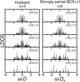
Figure 1: Local density of states (LDOS) for the Hubbard model ($\Delta=0$) and the strongly-paired BCS+$U$ model ($t=0$) at half filling as a function of on-site repulsive interaction, $U$. In the plot, $D=4t$ and $D_{\Delta}=4\Delta$.

For results, we first compute the local density of states (LDOS) for the strongly-paired BCS+$U$ model with $\varepsilon_{\bf k}=0$, which is a meaningful model at half filling since, in the large-$U$ limit, this model is precisely identical to the Heisenberg model Park . Figure 1 presents the comparison between the LDOS for this model and that for the Hubbard model (i.e., $\Delta_{\bf k}=0$), which shows that the two models have the almost identical local physics despite the difference that, at small $U$, the former has superconductivity and the latter does not. In fact, this local similarity is rather important and assuring since it suggests that the DMFT framework can capture not only the fundamental equivalence between the two models in the large $U$ limit, but also their close relationship at general $U$. It is emphasized that, as a function of $U$, the pairing term alone generates the self-energy correction practically identical to that of the Hubbard model.

Two facts are important to understand the nature of the insulating transition at large $U$. First, it is shown in our DMFT calculation that the anomalous self-energy correction in fact vanishes, eliminating the possibility of odd-frequency pairing. While at half filling this fact can be deduced rather straightforwardly by using (i) the particle-hole symmetry and (ii) the $d$-wave pairing symmetry, the situation is less clear at finite doping. It is only through explicit numerical computation that the anomalous self-energy correction is shown to become zero due to intricate adjustment of relevant parameters in the effective impurity-bath Hamiltonian in Eq. (21).

Second, $\Sigma(i\omega)$ becomes a linear function of $i\omega$ in the low-energy limit, at least, within the metallic regime: $\Sigma\simeq U/2+(1-1/Z)i\omega$. Note that the constant term of the normal self-energy exactly cancels the chemical potential at half filling. In this case the denominator of the normal Green’s function simply becomes $\omega^{2}/Z^{2}-\Delta^{2}_{\bf k}$ after the analytic continuation of $i\omega\rightarrow\omega+i\delta$ since the denominator of $G(i\omega)$ is $|i\omega-\varepsilon_{c}-\Sigma(i\omega)|^{2}+\Delta^{2}_{\bf k}$ when the anomalous self-energy correction is zero. In the above, the core energy, $\varepsilon_{c}$ $(=-\mu)$, is $-U/2$ at half filling. The pole structure at $\omega=\pm Z|\Delta_{\bf k}|$ indicates that the pairing dispersion is effectively renormalized to be $Z\Delta_{\bf k}$. As implied in Fig. 1, $Z$ decreases as a function of $U$ and finally vanishes at a critical value, $U_{c}$, inducing the collapse of superconductivity. Therefore, in our DMFT framework, $Z$ contains the major effect of superconducting fluctuations.

It is interesting to note that the strongly-paired BCS+$U$ model shows no gap structure in the local density of states. Instead, this model exhibits the characteristic Kondo resonance peak similar to that of the Hubbard model. We emphasize that in the above $\Sigma(i\omega)$ is generated solely from the $d$-wave pairing term in the presence of $U$. In the general BCS+$U$ model where both $t$ and $\Delta$ are not zero, the self-energy corrections from the both terms mix, which in turn shifts $U_{c}$ from that of the pure Hubbard model (or equivalently that of the strongly-paired BCS+$U$ model). Also, the existence of finite $\Delta/t$ shows up as sharp superconducting coherence peaks in the local density of states. We discuss this problem in the next section.

IV.2 Superconductor-to-insulator transition in the BCS+$U$ model

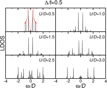
Figure 2: Local density of states (LDOS) for the BCS+$U$ model with $\Delta/t=0.5$ at half filling as a function of $U$. $\Delta$ denotes the bare pairing amplitude and $D(=4t)$ indicates half the bare band width. The dotted curve in the top, left panel indicates the LDOS analytically obtained for the non-interacting system with $U/D=0$.

Figure 2 plots the LDOS for the BCS+$U$ Hamiltonian with $\Delta/t=0.5$ at half filling as a function of $U$. Due to pairing, the density of states is reduced in the vicinity of the Fermi level (i.e., near $\omega/D=0$ in the plot) and the coherence peak develops at the position of basically the superconducting energy gap. What is most important in Fig. 2 (and also in Fig. 4) is that the superconducting gap closes as $U$ increases, and eventually disappears for $U/D\gtrsim 3.5$. (Note that, despite its discrete nature, the highest LDOS peak near the Fermi level can be taken to be a good indicator for the real coherence peak in the continuum limit, as demonstrated in the top, left panel of Fig. 2.) It is important to note that the bare pairing amplitude is set to be constant. Since the bare pairing amplitude is physically equivalent to the energy gap for singlet formation Park ; PRT ; ALRTZ , the large renormalization of the bare pairing amplitude provides an explanation for the pseudogap phenomenon. That is to say, at half filling, the real superconducting gap is strongly renormalized from the bare pairing amplitude and finally becomes zero in the large $U$ limit. So, superconductivity is hidden at half filling while singlet pairs are inherently present due to the non-zero bare pairing amplitude.

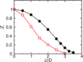
Figure 3: Quasiparticle spectral weight, Z, as a function of $U$. Solid circles indicate $Z$ of the BCS+$U$ model with $\Delta/t=0.5$ while empty squares denote that of the Hubbard model. The error bar due to the fitting procedure necessary for determining $Z$ from the low-energy behavior of $\Sigma(i\omega)$ is estimated to be smaller than the size of the symbol. Note that, since the above calculation is performed at zero temperature, we ignore the second DMFT solution which is adiabatically connected to the insulating phase generating smaller $Z$ DMFT_review . At zero temperature this second solution is higher in energy than the metallic (superconducting) solution.

As mentioned in the previous section, the superconductor-to-insulator transition is driven by the collapse of the quasiparticle spectral wight, $Z$. It is shown also in the previous section that $Z$ of the strongly-paired BCS+$U$ model (i.e., when $\Delta/t\rightarrow\infty$) has the $U$ dependence almost identical to that of the pure Hubbard model. When $\Delta/t$ is finite, however, the self-energy corrections from the hopping and pairing term mix and thus $Z$ is modified. Figure 3 plots $Z$ of the BCS+$U$ model with $\Delta/t=0.5$ in comparison to that of the Hubbard model. As seen in the plot, $Z$ is modified so that it is enhanced for a given $U$, leading to an increased $U_{c}$. It is interesting to observe that, when coexisting with the hopping term, the pairing correlation reduces the effect of $U$ and delays the insulating phase transition.

It has been shown so far in this section that superconductivity is suppressed for sufficiently large $U$ at half filling. A natural question that follows is if superconductivity can actually reemerge when electrons become mobile upon doping. Before addressing this issue in Sec. IV.4, however, we first investigate the second kind of the pseudogap phenomenon which is associated with the local phase coherence.

IV.3 Local phase stiffness and the pseudogap

We first need to quantify the local phase coherence. Fortunately, our DMFT formalism renders a very natural way to measure the local phase coherence by implementing a twist in local phase. The superconducting phase of a locally coherent region (which includes a given site and its correlated surroundings) can be twisted by performing $W_{l}\rightarrow W_{l}e^{i\theta}$ for every $l$, while the superconducting phase of the bath, $\tilde{\Delta}_{l}$, remains fixed. In other words, the anomalous hybridization between a given site and every bath orbital connected to it is twisted in phase.

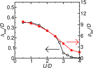
Figure 4: $U$ dependence of the renormalized superconducting gap, $\Delta_{\textrm{ren}}$ (empty circles), and the local phase stiffness, $\rho_{\textrm{loc}}$ (solid squares), at half filling. $\Delta_{\textrm{ren}}$ is determined to be the position of the coherence peak in the local density of states. $\rho_{\textrm{loc}}$ is computed from the energy cost of local phase twist. Note that the bare pairing amplitude is constant: $\Delta/t=0.5$.

To see what this phase twist entails, let us consider its effects on the Weiss field in Eq. (34), which describes the dynamics of the impurity electron after integrating out the bath. In particular, $\Gamma(i\omega)$ and $\Lambda(i\omega)$ in Eq. (35) are transformed as follows:

$$\Gamma(i\omega)= \sum_{l}\Big{(}V^{2}_{l}G_{l}-W^{2}_{l}G^{*}_{l}+2V_{l}W_{l}F_{l}\cos{\theta}\Big{)},$$

$$\Lambda(i\omega)= \sum_{l}\Big{[}(V^{2}_{l}-W^{2}_{l}e^{2i\theta})F_{l}-V_{l}W_{l}e^{i\theta}(G_{l}+G^{*}_{l})\Big{]}.$$ (37)

Apparently, the effective impurity action is not generally invariant under the local phase twist. In the special case of the $d$-wave superconducting bath, however, it turns out that the impurity action is actually invariant owing to the fact that $\sum_{l}V_{l}W_{l}F_{l}=0$ and $\Lambda(i\omega)=0$ for all $\omega$. Note that $\sum_{l}V_{l}W_{l}F_{l}=0$ due to the $d$-wave pairing symmetry and $\Lambda(i\omega)=0$ due to the absence of odd-frequency pairing. Consequently, eigenenergies are also invariant. However, since the ground state itself is rotated, there is an energy cost of the rotated ground state against the original Hamiltonian once the phase rotation symmetry is spontaneously broken. This energy cost can be computed as follows:

$$\Delta E(\theta)=\langle\Psi_{\theta}|H_{\textrm{i-b}}|\Psi_{\theta}\rangle-E_{0}$$ (38)

where $|\Psi_{\theta}\rangle$ is the ground state wave function at the phase twist of $\theta$, $H_{\textrm{i-b}}$ is the effective impurity-bath Hamiltonian at $\theta=0$, and $E_{0}$ is the ground state energy at $\theta=0$.

The local phase stiffness, $\rho_{\textrm{loc}}$, is defined as the curvature of the energy cost with respect to the local phase twist: $\Delta E\simeq\rho_{\textrm{loc}}\theta^{2}/2$ for sufficiently small $\theta$. Figure 4 shows the $U$ dependence of $\rho_{\textrm{loc}}$ in comparison with that of the renormalized superconducting gap, $\Delta_{\textrm{ren}}$, which is defined as the position of the coherence peak in Fig. 2. It is important to note that, for $U/D\gtrsim 3.5$, the superconducting coherence peak completely disappears while the local phase stiffness remains finite. This disparity is the essence of the pseudogap phenomenon associated with the local phase coherence.

IV.4 Reemergence of superconductivity at finite doping

We now turn to the doped BCS+$U$ model. As demonstrated in Fig. 4, the superconducting gap is suppressed at half filling for sufficiently large $U/D$. The question is whether hidden superconductivity can reemerge when phase fluctuations are lessened by allowing charge fluctuations via doping. Figure 5 shows that the increase in hole concentration indeed gradually opens up the superconducting gap at the Fermi level of $\omega/D=0$. It is interesting to observe the specific route in which the superconducting gap is opened up. As the hole concentration increases, the lower Hubbard band moves toward the Fermi level and provides a necessary density of states for suppressed superconductivity to become reactivated.

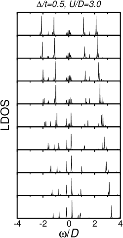
Figure 5: Local density of states (LDOS) for the BCS+$U$ model with $\Delta/t=0.5$ and $U/D=3$ as a function of doping. The value of $U/D=3$ is chosen so that the ground state at half filling is just about to enter the insulating phase, which corresponds to the almost fully Gutzwiller-projected regime. The top panel plots the LDOS at half filling which is obtained when $\mu=\mu_{0}\equiv U/2$. From the top to bottom panels, the chemical potentials (the corresponding hole concentration, $x$) are $\mu_{0}$ ($0\%$), $0.9\mu_{0}$ ($1.65\%$), $0.8\mu_{0}$ ($3.70\%$), $0.7\mu_{0}$ ($6.42\%$), $0.6\mu_{0}$ ($9.90\%$), $0.5\mu_{0}$ ($14.10\%$), $0.4\mu_{0}$ ($19.30\%$), $0.3\mu_{0}$ ($25.13\%$), and $0.2\mu_{0}$ ($31.53\%$), respectively.

Note that $\Delta/t=0.5$ is an appropriate value for the $t$-$J$ model in the regime of exchange coupling $J/t\simeq 0.5-1.0$ and hole concentration $x\simeq 10-15\%$ (optimal doping). As mentioned in Sec. II, such connection between the $t$-$J$ model and the Gutzwiller-projected BCS model is established via wave function overlap using exact diagonalization Park . Therefore, in Fig. 5 the fifth or sixth panel from the top corresponds to the actual local density of states of the $t$-$J$ model in the regime specified in the above. It will be interesting for future work to conduct a systematic survey of the renormalized superconducting gap as a function of doping, obtained from the bare pairing amplitude properly determined from exact diagonalization.

V Conclusion

In this paper, the dynamical mean field theory is used for the analysis of the BCS+$U$ Hamiltonian with $U$ imposing the (partial) Gutzwiller projection. Strong phase fluctuations at half filling are manifested through the collapse of the quasiparticle spectral weight, $Z$, which affects not only the quasiparticle effective mass, but also the pairing amplitude. As a consequence, the distance between the superconducting coherence peaks in the density of states (which measures the renormalized superconducting gap) decreases at the same time as the overall weight is reduced. It is thus fundamentally due to strong phase fluctuations that the renormalized superconducting gap decreases as a function of $U$ and finally vanishes for a given finite bare pairing amplitude.

Moreover, it is shown that the local phase coherence can survive even after the global phase coherence identified with the sharp superconducting coherence peak is lost. Combined with this result for the local phase coherence, the collapse of the renormalized superconducting gap provides an explanation for the pseudogap phenomenon. That is, there are two different pseudogap energy scales, one of which is associated with the bare pairing amplitude that can remain finite even at half filling. The other is associated with the local phase stiffness that vanishes at sufficiently small doping in the large $U$ limit. In this view, the real superconducting gap is given by the fully renormalized pairing gap which is the smallest energy scale at small doping for finite $U$ and vanishes faster than the other two energy scales as $U$ increases. It is further shown that hidden superconductivity at half filling can indeed reemerge upon doping, as indicated by the reappearance of the superconducting coherence peaks in the density of states.

We finally conclude by putting our theory in perspective. Obviously, it is well beyond the scope of this paper to provide a complete review of previous theories on the pseudogap phenomena. Thus, we select only a few theories that are closely related to our theory. In an overall scheme our theory can be categorized as the theory with preformed pairs since electron pairs are inherently present due to the bare pairing amplitude. There are, however, many variations in the theory of preformed-pair scenario. Pairs can be preformed by (i) the spin-charge separation KotliarLiu ; LeeNagaosa ; LeeWen involving deconfined phases LeeNagaosaWen , (ii) the formation of microscopic stripes Stripe , (iii) the proximity to the long-range antiferromagnetic order MMP (or the nearly antiferromagnetic Fermi liquid theory), and so on. In our theory, preformed pairs exist because the ground state itself has the bare pairing amplitude due to the fundamental connection between the $t$-$J$ model and the projected BCS Hamiltonian. The dichotomy between the bare and real superconducting gap originates from the strong renormalization effect of large on-site repulsive interaction, $U$.

It is interesting to note that the above-mentioned theories including ours can be categorized further into two classes, as proposed by Lee, Nagaosa, and Wen. In their review paper LeeNagaosaWen , Lee et al. coined the words, “thermal explanation” and “quantum explanation” of the pseudogap. The quantum explanation of the pseudogap proposes a fundamentally new quantum state which, for example, is the deconfined spin-liquid phase in the above spin-charge separation scenario. Despite the fact that this deconfined spin-liquid state may be unstable in the square-lattice $t$-$J$ model, it is assumed that the pseudogap is a high-frequency property of the spin-liquid phase, seen at high temperature.

On the other hand, the thermal explanation refers to any theories viewing the pseudogap as a finite-temperature manifestation of the spin gap necessary for the formation of singlet pairs, which is induced fundamentally by the symmetry-breaking ground state at zero temperature. Broken symmetries are the lattice translation, spin rotation, and global gauge invariance in the case of the stripe theory, the nearly antiferromagnetic Fermi liquid theory, and the fluctuating superconductivity theory EmeryKivelson (which conceptually includes our theory of the Gutzwiller-projected BCS model), respectively. The main difference between our theory and the others is that the real superconducting gap originates from the same spin gap while it is strongly renormalized due to large $U$. Consequently, in our theory, only the real superconducting gap is shown in the zero-temperature density of states while a signature for the pseudogap can be seen in the finite-temperature counterpart.

Acknowledgments

The author is grateful to Y. Bang, H.-Y. Choi, G. S. Jeon, and K.-S. Kim for their insightful comments.

References

- (1) P. A. Lee, N. Nagaosa, and X.-G. Wen, Rev. Mod. Phys. 78, 17 (2006).
- (2) T. Timusk and B. Statt, Rep. Prog. Phys. 62, 61 (1999).
- (3) N. J. Curro, T. Imai, C. P. Slichter, and B. Dabrowski, Phys. Rev. B 56, 877 (1997).
- (4) J. W. Loram, K. A. Mirza, J. R. Cooper, and W. Y. Liang, Phys. Rev. Lett. 71, 1740 (1993).
- (5) M. R. Norman, H. Ding, M. Randeria, J. C. Campuzano, T. Yokoya, T. Takeuchi, T. Takahashi, T. Michiku, K. Kadowaki, P. Guptasarma, and D. Hinks, Nature (London) 392, 157 (1998).
- (6) C. C. Homes, T. Timusk, R. Liang, D. A. Bonn, and W. N. Hardy, Phys. Rev. Lett. 71, 1645 (1993).
- (7) V. J. Emery and S. Kivelson, Nature (London) 374, 434 (1995).
- (8) Z. A. Xu, N. P. Ong, Y. Wang, T. Kakeshita, and S. Uchida, Nature (London) 406, 486 (2000).
- (9) K. Park, Phys. Rev. Lett. 95, 027001 (2005); Phys. Rev. B 72, 245116 (2005).
- (10) P. W. Anderson, Science 235, 1196 (1987).
- (11) A. Georges, G. Kotliar, W. Krauth, and M. J. Rozenberg, Rev. Mod. Phys. 68, 13 (1996).
- (12) B. Kyung and A.-M. S. Tremblay, Phys. Rev. Lett. 97, 046402 (2006).
- (13) M. Capone and G. Kotliar, Phys. Rev. B 74, 054513 (2006).
- (14) D. Poilblanc and D. J. Scalapino, Phys. Rev. B 66, 052513 (2002).
- (15) Y. Ohta, T. Shimozato, R. Eder, and S. Maekawa, Phys. Rev. Lett. 73, 324 (1994).
- (16) M. Caffarel and W. Krauth, Phys. Rev. Lett. 72, 1545 (1994).
- (17) A. Paramekanti, M. Randeria, and N. Trivedi, Phys. Rev. Lett. 87, 217002 (2001).
- (18) P. W. Anderson, P. A. Lee, M. Randeria, N. Trivedi, and F. C. Zhang, J. Phys.: Condens. Matter 16, R755 (2004).
- (19) G. Kotliar and J. Liu, Phys. Rev. B 38, 5142 (1988).
- (20) P. A. Lee and N. Nagaosa, Phys. Rev. B 46, 5621 (1992).
- (21) P. A. Lee and X.-G. Wen, Phys. Rev. Lett. 78, 4111 (1997).
- (22) V. J. Emery, S. A. Kivelson, and O. Zachar, Phys. Rev. B 56 6120 (1997).
- (23) A. J. Millis, H. Monien, and D. Pines, Phys. Rev. B 42 167 (1990).