GRANULAR GAS COOLING AND RELAXATION TO THE STEADY STATE IN REGARD TO THE OVERPOPULATED TAIL OF THE VELOCITY DISTRIBUTION

Abstract

We present a universal description of the velocity distribution function of granular gases, $f(v)$, valid for both, small and intermediate velocities where $v$ is close to the thermal velocity and also for large $v$ where the distribution function reveals an exponentially decaying tail. By means of large-scale Monte Carlo simulations and by kinetic theory we show that the deviation from the Maxwell distribution in the high-energy tail leads to small but detectable variation of the cooling coefficient and to extraordinary large relaxation time.

PACS Nos.: 47.70.-n, 51.10.+y

1 Introduction

Granular gases are characterized by a certain loss of kinetic energy according to the dissipative properties of particle collisions. The particle velocities before a collision, $\vec{v}_{1/2}$, and after, $\vec{v}_{1/2}^{\,\prime}$, are related by the collision rule

$$\vec{v}_{1}^{\,\prime} =\vec{v}_{1}-\frac{1+\varepsilon}{2}\left(\vec{v}_{12}\cdot\vec{e}\,\right)\vec{e}$$ (1)

$$\vec{v}_{2}^{\,\prime} =\vec{v}_{2}+\frac{1+\varepsilon}{2}\left(\vec{v}_{12}\cdot\vec{e}\,\right)\vec{e}$$

with $\vec{v}_{12}\equiv\vec{v}_{1}-\vec{v}_{2}$ and the unit vector $\vec{e}\equiv\left(\vec{r}_{1}-\vec{r}_{2}\right)/\left|\vec{r}_{1}-\vec{r}_{2}\right|$ at the moment of the collision.

In the absence of external excitation, a homogeneously initialized granular gas stays homogeneous during the first part of its evolution, called homogeneous cooling state (HCS). In later stages of its evolution, hydrodynamics instabilities develop leading to vortex formation, that is, spacial correlations of the vectorial velocity field,[1] and finally cluster formation due to a pressure instability.[2] In this paper we restrict ourselves to the homogeneous cooling state. It should be mentioned that heated granular gases with a Gaussian thermostat are equivalent to the HCS[3], therefore, the presented results apply also for such systems.

According to the steady loss of energy, the velocity distribution function, $f\left(\vec{v},\tau\right)$, depends on time $\tau$ (measured in units of collisions per particle). Its shape can be described by the time-independent function $\tilde{f}(\vec{c}\,)$ via[4]

$$f\left(\vec{v},\tau\right)=\frac{n}{v_{T}^{3}(\tau)}\tilde{f}\left(\vec{c}\,\right)$$ (2)

where

$$\vec{c}\equiv\frac{\vec{v}}{v_{T}(\tau)}\qquad\mbox{and}\qquad v_{T}(\tau)\equiv\sqrt{2T(\tau)}\,.$$ (3)

The evolution of the granular temperature $T(\tau)$ is given by Haff’s law[5] (with particle mass $m_{i}=1$),

$$\frac{dT}{d\tau}=-2\gamma T\,,~{}~{}~{}~{}\mbox{i.e.,}\,~{}~{}~{}~{}~{}T(\tau)=T(0)\exp(-2\gamma\tau)\,.$$ (4)

Here $\gamma$ is the cooling coefficient, addressed in detail in the next section.

2 Universal velocity distribution function

For small and intermediate velocities, $\left|\vec{v}\right|\approx v_{T}$, that is, $\left|\vec{c}\,\right|\approx 1$, the scaled velocity distribution function $\tilde{f}(\vec{c}\,)$ is close to a Gaussian with small deviations that can be characterized by the first non-trivial coefficient, $a_{2}$, of a Sonine polynomials expansion around the leading Gauss distribution,[6, 7]

$$\tilde{f}(c)=\pi^{-3/2}\exp\left(-c^{2}\right)\left[1+a_{2}S_{2}\left(c^{2}\right)\right]~{}~{}~{}~{}\mbox{with}~{}~{}~{}~{}S_{2}\left(c^{2}\right)=\frac{1}{1}c^{4}-\frac{5}{2}c^{2}+\frac{15}{8}\,$$ (5)

and

$$a_{2}(\varepsilon)=\frac{16(1-\varepsilon)\left(1-2\varepsilon^{2}\right)}{81-17\varepsilon+30\varepsilon+30^{2}(1-\varepsilon)}\,.$$ (6)

For large kinetic energy, $c\gg 1$, the distribution function decays exponentially slow, that is, the distribution function is overpopulated with respect to the Gauss distribution one would expect for a molecular gas,[4, 7]

$$\tilde{f}(c)=Be^{-bc}\,~{}~{}~{}~{}~{}\mbox{with}~{}~{}~{}~{}~{}~{}b=\frac{3\pi}{\mu_{2}}$$ (7)

with the second moment of the dimensionless collision integral

$$\mu_{2}\equiv-\int d\vec{c}_{1}c_{1}^{2}\tilde{I}\left(\tilde{f},\tilde{f}\right)=\sqrt{2\pi}\left(1-\varepsilon^{2}\right)\left[1+\frac{3}{16}a_{2}\right]$$ (8)

and with

$$\tilde{I}\left(\tilde{f},\tilde{f}\right)=\int d\vec{c}_{2}\int d\vec{e}\,\,\Theta\!\left(-\vec{c}_{12}\cdot\vec{e}\,\right)\left|\vec{c}_{12}\cdot\vec{e}\,\right|\left[\frac{1}{\varepsilon^{2}}\tilde{f}\left(\vec{c}_{1}^{\,\prime\prime}\right)\tilde{f}\left(\vec{c}_{2}^{\,\prime\prime}\right)-\tilde{f}\left(\vec{c}_{1}\right)\tilde{f}\left(\vec{c}_{2}\right)\right]$$ (9)

where $\vec{c}_{1/2}^{\,\prime\prime}$ are the pre-collisional scaled velocities.

There is a transition region between the ranges of validity of the Sonine expansion ($c\approx 1$) and the expression for the tail ($c\gg 1$) where the distribution function was quantified in terms of complicated implicit expressions.[8] For practical computations, however, a much simpler approach may be sufficient: It was shown recently that the simple combination of the shown Sonine expansion and the exponential tail,

$$\tilde{f}(c)=\left\{\begin{aligned} Ac^{2}e^{-c^{2}}\left[1+a_{2}S_{2}(c^{2})\right]&\mbox{~{}~{}~{}~{}for}&c<c_{*}\\ Bc^{2}e^{-bc}&\mbox{~{}~{}~{}~{}for}&c\geq c_{*}\end{aligned}\right.$$ (10)

with the parameters $A$, $B$, and the transition velocity $c_{*}$ agrees with large-scale DSMC simulation up to a very good accuracy in the entire range of velocities.[9] The parameters $A$, $B$, and $c_{*}$ follow from the conditions of smoothness

$$\tilde{f}(c_{*}+0) =\tilde{f}(c_{*}-0)$$ (11)

$$\left.\frac{d\tilde{f}}{dc}\right|_{c_{*}+0} =\left.\frac{d\tilde{f}}{dc}\right|_{c_{*}-0}$$

and normalization:

$$c_{*} = \frac{b}{2}+\frac{a_{2}\left(2c_{*}^{3}-5c_{*}\right)}{2\left[1+a_{2}S_{2}\left(c_{*}^{2}\right)\right]}$$ (12)

$$\frac{1}{A} = \frac{k(c_{*})}{b^{3}}\!\left[2+bc_{*}\left(2\!+\!bc_{*}\right)\right]e^{-bc_{*}}\!+\!\frac{\sqrt{\pi}}{4}{\rm Erf}(c_{*})\!-\!\frac{c_{*}}{8}\!\left[4\!+\!a_{2}c_{*}^{2}\!\left(2c_{*}^{2}\!-\!5\right)\right]\!e^{-c_{*}^{2}}$$ (13)

$$B = Ak(c_{*})$$ (14)

with

$$k(c_{*})\equiv e^{-c_{*}^{2}+bc_{*}}\left[1+a_{2}S_{2}\left(c_{*}^{2}\right)\right]\,.$$ (15)

Solving the fifth order equation (12) numerically for $c_{*}$, we obtain $A$, $k$ and finally $B$.[9]

3 Impact of the high-velocity tail on the coefficient of cooling

By means of the distribution function, Eq. (10), and its parameters $A$, $B$, $c_{*}$ depending on the coefficient of restitution $\varepsilon$, we can quantify the impact of the exponential tail on the cooling coefficient $\gamma$, which is one of the most important characteristics of a granular gas. Using the standard analysis,[10] one can calculate the cooling coefficient for the homogeneous cooling state, when the stationary velocity distribution is achieved:

$$\gamma=\left(1-\varepsilon^{2}\right)\frac{J_{2}}{12J_{0}}\,,$$ (16)

where the coefficients $J_{k}$ depend on the velocity distribution function,

$$J_{k}=\int d\vec{c}_{1}d\vec{c}_{2}\int d\vec{e}\,\Theta(-\vec{c}_{12}\cdot\vec{e}\,)|\vec{c}_{12}\cdot\vec{e}\,|^{k+1}\tilde{f}(c_{1})\tilde{f}(c_{2})\,.$$ (17)

If we neglect the exponential tail, we obtain the energy decay rate[7]

$$\gamma_{0}(\varepsilon)=\frac{1-\varepsilon^{2}}{6}\frac{1+\frac{3}{16}\,a_{2}(\varepsilon)}{1-\frac{1}{16}\,a_{2}(\varepsilon)}\,.$$ (18)

Complementary, we determine the cooling coefficient numerically, using Direct Simulation Monte Carlo (DSMC)[11, 12]. We initialized a granular gas of $N=10^{8}$ particles with velocities drawn from a Gauss distribution at $T(0)=1$ and simulated until the particle velocities reached the limit of the double precision number representation, i.e., until $T\approx 10^{-23}$. For $\varepsilon=0.9$ this corresponds to a total of $5\times 10^{10}$ collisions or 1,000 collisions per particle.

For different $\varepsilon$ we recorded the temperature $T_{\rm DSMC}(\tau)$. Then $\gamma_{\rm DSMC}$ was determined by fitting $T_{\rm DSMC}(\tau)$ for $\tau\gg 1$ to its asymptotic law, $T_{\rm DSMC}\propto\exp(-2\,\gamma_{\rm DSMC}\,\tau)$, Eq. (4).

The dependence of $\gamma_{0}$ on the coefficient of restitution $\varepsilon$ is shown in Fig. 1 together with the numerical result.

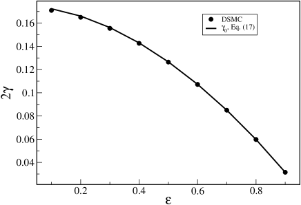
Figure 1: The cooling coefficient $\gamma(\varepsilon)$ as a function of the coefficient of restitution as obtained by Direct Simulation Monte Carlo (DSMC) (points) and due to Eq. (18), $\gamma_{0}$.

The numerical results (see below) and the theoretical results disregarding the tail, Eq. (18), virtually coincide. When we plot the difference of both curves, however, we find a systematic deviation between the numerical values and the analytical result (Fig. 2).

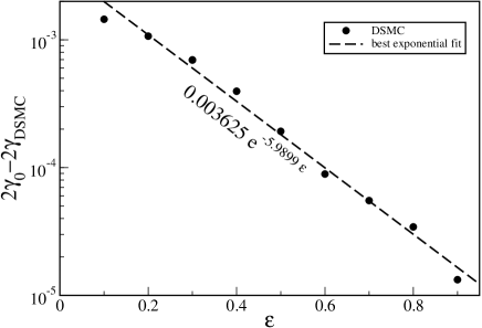
Figure 2: Difference of the cooling coefficient due to Eq. (18) and the numerically values, $(\gamma_{0}-\gamma_{\rm DSMC})$, over the coefficient of restitution. Since Eq. (18) disregards the exponential tail of the distribution, the shown difference is due to the presence of the tail. The dashed line shows the best exponential fit.

To estimate this rather small difference quantitatively, we write the distribution function as a sum of two terms,

$$\tilde{f}(c)=\tilde{f}_{0}(c)+\tilde{f}_{\rm t}(c)\,,$$ (19)

that is, the main part $\tilde{f}_{0}(c)$ (with $c$ extended to infinity), and the pure overpopulation of the tail, $\tilde{f}_{t}(c)$,

$$\tilde{f}_{0}(c)=Ac^{2}e^{-c^{2}}\left[1+a_{2}S_{2}\left(c^{2}\right)\right]$$ (20)

$$\tilde{f}_{t}(c)=\left[Bc^{2}\exp(-b\,c)-\tilde{f}_{0}(c)\right]\Theta\left(c-c_{*}\right)\,.$$ (21)

The product $\tilde{f}(c_{1})\tilde{f}(c_{2})$ in Eq. (17) reads then

$$\tilde{f}(c_{1})\tilde{f}(c_{2})=\tilde{f}_{0}(c_{1})\tilde{f}_{0}(c_{2})+\tilde{f}_{0}(c_{1})\tilde{f}_{\rm t}(c_{2})+\tilde{f}_{\rm t}(c_{1})\tilde{f}_{0}(c_{2})+\tilde{f}_{\rm t}(c_{1})\tilde{f}_{\rm t}(c_{2})\,.$$

For large $c_{*}$ one can neglect the last term in the above equation. Moreover, in this case we approximate $\tilde{f}_{\rm t}(c)\approx B\exp(-b\,c)$ and $\vec{c}_{12}\cdot\vec{e}\approx\vec{c}_{1}\cdot\vec{e}$, assuming $c_{1}\gg c_{2}$. A similar approximation may be applied for the opposite case, $c_{2}\gg c_{1}$. Taking then into account the symmetry of the integrand in Eq. (17) with respect to $\vec{c}_{1}$ and $\vec{c}_{2}$, we finally obtain an estimate for $J_{k}$:

$$J_{k} =\frac{\pi}{16}A^{2}J_{k}^{(0)}+2\left[\int d\vec{c}_{2}\tilde{f}_{0}(c_{2})\right]\int d\vec{c}_{1}\int d\vec{e}\,\,\Theta(-\vec{c}_{1}\cdot\vec{e}\,)\left|\vec{c}_{1}\cdot\vec{e}\,\right|^{k+1}\tilde{f}_{\rm t}(c_{1})$$ (22)

$$=\frac{\pi}{16}A^{2}J_{k}^{(0)}+2A\frac{\sqrt{\pi}}{4}\,4\pi\int_{c_{*}}^{\infty}c_{1}^{k+3}Be^{-bc_{1}}dc_{1}2\pi\int_{\frac{\pi}{2}}^{\pi}\sin\theta\left|\cos\theta\right|^{k+1}\,,$$

where $J_{k}^{(0)}$ is the value of the coefficient $J_{k}$ for the distribution function $\tilde{f}_{0}(c)$ with $A$ in Eq. (20) equal to $4/\sqrt{\pi}$, that is, for the case when the exponential tail is disregarded. In particular, we need

$$J_{0}^{(0)} =2\sqrt{2\pi}\left(1-\frac{1}{16}a_{2}\right)$$ (23)

$$J_{2}^{(0)} =4\sqrt{2\pi}\left(1+\frac{3}{16}a_{2}\right)\,.$$

Performing the integration in Eq. (22) we obtain

$$J_{k}=\frac{\pi}{16}A^{2}J_{k}^{(0)}+\frac{\sqrt{\pi}}{4}\frac{2AB}{(k+2)}\frac{8\pi^{2}}{b^{k+4}}\Gamma(k+4,bc_{*})\,,$$ (24)

where $\Gamma(x,y)$ is the incomplete gamma-function. Inserting into Eq. (16) yields the cooling rate,

$$\gamma=\frac{(1-\varepsilon^{2})}{6}\,\frac{\left(1+\frac{3}{16}a_{2}\right)Ab^{6}+2\pi\sqrt{2}B\Gamma(6,bc_{*})}{\left(1-\frac{1}{16}a_{2}\right)Ab^{6}+8\pi\sqrt{2}Bb^{2}\Gamma(4,bc_{*})}\,.$$ (25)

Naturally, for $B=0$, corresponding to absence of the tail (see Eq. (10)), Eq. (25) reduces to the previous relation Eq. (18). In Fig. 3 the difference $(\gamma_{0}-\gamma)$ which quantifies the contribution to the cooling coefficient from the tail is compared with the numerical results.

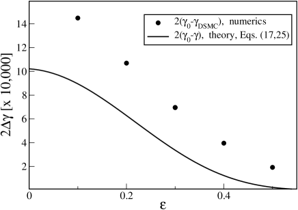
Figure 3: Influence of the tail on the cooling coefficient. The symbols show the same data as in Fig. 2 (but in linear scale). The full line shows $2(\gamma_{0}-\gamma)$ as given by Eqs. (18) and (25).

The scaling law, $\gamma_{0}-\gamma_{\rm DSMC}\propto\exp(-6\varepsilon)$, shown in Fig. 2 as a numerical result is, however, difficult to confirm analytically. The approximate analytical theory shown in Fig. 3 agrees with the numerical results only qualitatively.

4 Slow relaxation of the velocity distribution

In the above analysis we assumed that the velocity distribution function $\tilde{f}(c)$ had already relaxed to its steady state scaling shape. In our numerical experiments we observed, however, that the relaxation to the stationary form occurs extremely slowly, as compared to the relaxation of molecular gases to equilibrium distribution. To study this retarded relaxation quantitatively, we use the coefficient $\gamma_{\rm DSMC}$ described above, and define the temperature $T_{\rm fit}(\tau)\propto\exp(-2\gamma_{\rm DSMC}\,\tau)$. By definition, for $\tau\gg 1$ one obtains $T_{\rm DSMC}\approx T_{\rm fit}$ since $\gamma_{\rm DSMC}$ was determined as the best exponential fit to $T_{\rm DSMC}(\tau)$ for $\tau\gg 1$. Hence, the quantity $1-T_{\rm DSMC}(\tau)/T_{\rm fit}(\tau)$ characterizes the relaxation of the distribution function to its stationary form. We observe that the relaxation time depends sensitively on the coefficient of restitution $\varepsilon$.

Figures 4-7 illustrate the relaxation kinetics for different values of the coefficient of restitution $\varepsilon$. In Figs. 4 and 5 the initial relaxation is shown. We observe a initial quick relaxation with characteristic time of 3-5 collisions per particles, similar as for molecular gases.

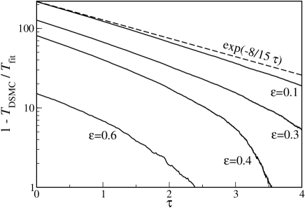
Figure 4: Short-time relaxation of the temperature decay to Haff’s law, Eq. (4) for a system of $N=10^{8}$ particles for different coefficients of restitution, $\varepsilon=0.1$, $\varepsilon=0.3$, $\varepsilon=0.4$, and $\varepsilon=0.6$. The initial relaxation occurs on the time scale $1-T_{\rm DSMC}/T_{\rm fit}\propto\exp(-8/15\tau)$.

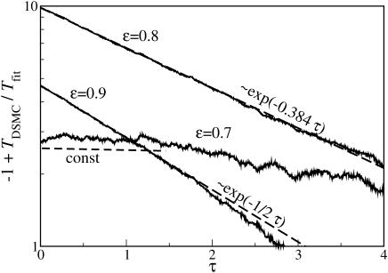
Figure 5: Same as Fig. 4 but for $\varepsilon=0.7$, $\varepsilon=0.8$, and $\varepsilon=0.9$. Note that the vertical axis has opposite sign as the axis in Fig. 4.

For values $\varepsilon<0.7$ the simulated temperature approaches Haff’s law from below (Fig. 4), whereas for $\varepsilon>0.7$ it approaches Haff’s law from above (note the different labeling of the vertical axis in these figures). For $\varepsilon=0.7$ the initial relaxation rate vanishes. This may be explained by the fact that at $\varepsilon\approx 0.7$ the value of the second Sonine coefficient changes its sign, see Eq. (6). That is, for $\varepsilon\lesssim 0.7$ the stationary velocity distribution $\tilde{f}$ is bent towards lower velocities as compared with the Maxwell distribution while for $\varepsilon\gtrsim 0.7$ the distribution is bent towards higher velocities. For $\varepsilon=0.7$ the second Sonine coefficient is very small, $a_{2}(0.7)\approx 0$, therefore, for $c\sim 1$ the distribution function is very close to the Maxwell distribution and, thus, there is no initial relaxation. These arguments prove that the initial relaxation shown in Figs. 4 and 5 corresponds to the relaxation of the main part of the velocity distribution, $c\sim 1$, whose deviation from the Maxwell distribution is described by the second Sonine coefficient $a_{2}$.

For small coefficient of restitution, $\varepsilon\leq 0.6$, the initial slope of the relaxation curves is almost independent of $\varepsilon$. Its value is surprisingly close to the slope $-8/15$ of the relaxation curve of the second Sonine coefficient in the limit of almost elastic particles, $\varepsilon\lesssim 1$.[10] Also surprisingly, for larger values of the restitution coefficients $\varepsilon>0.7$, which correspond to negative values of the second Sonine coefficient, the slope becomes smaller and depends noticeably on $\varepsilon$. For almost elastic particles, $\varepsilon=0.9$ we find the initial slope 1/2. Presently we do not have an explanation for this behavior of the initial relaxation.

In Figs. 6 and 7 we present the complete relaxation to the steady state.

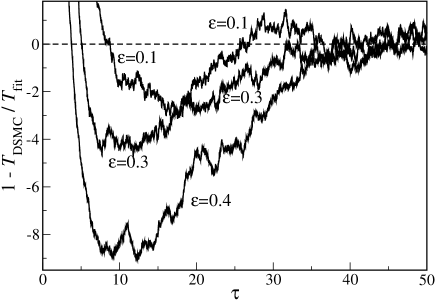
Figure 6: Long-time relaxation of the temperature decay rate for $\varepsilon=0.1$, $\varepsilon=0.3$, and $\varepsilon=0.4$.

Figure 7: Same as Fig. 6 but for $\varepsilon=0.6$, $\varepsilon=0.7$, $\varepsilon=0.8$, and $\varepsilon=0.9$.

The complete relaxation requires much longer time as compared to molecular gases. This is related to the relatively slow formation of the exponential tail. The relaxation time depends on the coefficient of restitution as shown in Fig. 6. The larger the coefficient of restitution the longer it takes to form the complete velocity distribution including the exponential tail.

To explain this effect we use the equation for the relaxation of the velocity distribution function to its scaling form,[10, 13]

$$\frac{\mu_{2}}{3}\left(3+c\frac{\partial}{\partial c}\right)\tilde{f}(c,\tau)+J_{0}\frac{\partial}{\partial\tau}\tilde{f}(c,\tau)=\tilde{I}\left(\tilde{f},\tilde{f}\right)$$ (26)

where $\tilde{I}(\tilde{f},\tilde{f})$ is the reduced collision integral, Eq. (9), and $J_{0}$ is given in Eq. (17). As usual we neglect the incoming term for $c\gg 1$[4, 7], leading to the approximation

$$\tilde{I}\left(\tilde{f},\tilde{f}\right)\approx-\pi c\tilde{f}(c)~{}~{}~{}~{}~{}\mbox{for}~{}~{}~{}~{}~{}c\gg 1\,.$$ (27)

With the Ansatz $\tilde{f}(c,\tau)=B\exp\left[-w(\tau)c\right]$ we recast Eq. (26) into

$$\frac{dw}{d\tau}+\frac{\mu_{2}}{3J_{0}}w=\frac{\pi}{J_{0}}~{}~{}~{}~{}~{}\mbox{for}~{}~{}~{}~{}~{}~{}c\gg 1\,$$ (28)

with the solution

$$w(\tau)=b+(1-b)\exp\left[-\frac{\tau}{\tau_{0}(\varepsilon)}\right]\,,$$ (29)

where $b=3\pi/\mu_{2}$ coincides with Eq. (7) and $\tau_{0}^{-1}(\varepsilon)=\mu_{2}/3J_{0}$. Neglecting $a_{2}$, which quantifies (small) deviations of the main part of the distribution with respect to the Maxwellian, and the contribution from the tail, Eq. (23) yields $J_{0}=2\sqrt{2\pi}$, which together with Eq. (8) leads to the relaxation time

$$\tau_{0}^{-1}(\varepsilon)=\frac{1-\varepsilon^{2}}{6}\,.$$ (30)

For example, for $\varepsilon=0.4$ we obtain the theoretical relaxation time, $\tau_{0}\approx 7.1$. As shown in Fig. 6 for $\varepsilon=0.4$ in the simulation the quantity $(1-T_{\rm DSMC}/T_{\rm fit})$ decreases by the factor of $10$ in the time span $\Delta\tau=25$, ranging from $\tau=10$ to $\tau=35$. This gives the estimate for the relaxation time $\tau_{0}=25/\log(10)\approx 10.8$, in agreement with the above theoretical value $\tau_{0}=7.1$.

From the above theory we expect that the relaxation time increases with $\varepsilon$. While this tendency is confirmed for small coefficients of restitution from $\varepsilon=0.1$ to $\varepsilon=0.4$, Fig. 6, the relaxation time seems to saturate for larger $\varepsilon\geq 0.6$, Fig. 7. This is, presumably, a finite size effect: For large values of $\varepsilon$ the number of particles in the tail, which is determined by the threshold velocity $c_{*}$, increasing with $\varepsilon$, is not large enough to develop a significant tail. Therefore for such systems the apparent relaxation occurs much faster then it would be in a sufficiently large system. The relaxation time is mainly determined by the number of particles in the tail, rather then by the coefficients of restitution $\varepsilon$. Nevertheless, even for these systems, which are not sufficiently large for a quantitative study of the tail relaxation, the latter occurs anomalously slow.

5 Conclusion

We studied analytically and numerically the impact of the high-energy tails of the velocity distribution function in granular gases in the homogeneous cooling state on the cooling coefficient and on the relaxation time towards the steady state velocity distribution.

In our analytical theory we used an universal Ansatz for the velocity distribution function for the entire range of velocities. This Ansatz comprises the main part of the distribution function, where the velocities are of the order of the thermal velocity, $v\sim v_{T}$ as well as the tail, where $v\gg v_{T}$.

We derived the coefficients of the proposed Ansatz, which allows to estimate the cooling coefficient and to characterize the impact of the high-energy tail on the cooling. Our analytical results are in qualitative agreement with numerical data obtained by Direct Simulation Monte Carlo of $10^{8}$ particles.

In the simulations we found anomalously slow relaxation of the velocity distribution function to its stationary form as compared to the relaxation of molecular gases, where the relaxation occurs during few collision times. Instead, for granular gases, we observed much longer relaxation, in the order of 20-30 collisions per particle. To explain this slow relaxation we developed a theory, which predicts that the relaxation time increases with decreasing inelasticity, in agreement with the numerical observations. For a large coefficient of restitution the relaxation time saturates with increasing $\varepsilon$, which may be attributed to finite size effects, that is, the system of $10^{8}$ particles is not large enough for the quantitative numerical analysis of the tail relaxation.

References

- [1] R. Brito, M. H. Ernst, Extension of Haff’s cooling law in granular flows, Europhys. Lett. 43 (1998) 497.
- [2] I. Goldhirsch, G. Zanetti, Clustering instability in dissipative gases, Phys. Rev. Lett. 70 (1993) 1619.
- [3] J. M. Montanero, A. Santos, Computer simulation of uniformly heated granular fluids, Granular Matter 2 (1999) 53–64.
- [4] S. E. Esipov, T. Pöschel, The granular phase diagram, J. Stat. Phys. 86 (1997) 1385.
- [5] P. K. Haff, Grain flow as a fluid-mechanical phenomenon, J. Fluid Mech. 134 (1983) 401.
- [6] A. Goldshtein, M. Shapiro, Mechanics of collisional motion of granular materials. Part 1: General hydrodynamic equations, J. Fluid Mech. 282 (1995) 75.
- [7] T. P. C. van Noije, M. H. Ernst, Velocity distributions in homogeneous granular fluids: the free and the heated case, Granular Matter 1 (1998) 57.
- [8] I. Goldhirsch, H. S. Noskowicz, O. Bar-Lev, The homogeneous cooling state revisited, in: T. Pöschel, N. V. Brilliantov (Eds.), Granular Gas Dynamics, Vol. 624 of Lecture Notes in Physics, Springer, Berlin, 2003, pp. 37 – 63.
- [9] T. Pöschel, N. V. Brilliantov, A. Formella, Impact of high-energy tails on granular gas properties, Phys. Rev. E 74 (2006) 041302.
- [10] N. V. Brilliantov, T. Pöschel, Kinetic Theory of Granular Gases, Oxford University Press, Oxford, 2004.
- [11] G. A. Bird, Molecular Gas Dynamics and the Direct Simulation of Gas Flows, Oxford University Press, 1994.
- [12] J. M. Montanero, A. Santos, Monte Carlo simulation method for the Enskog equation, Phys. Rev. E 54 (1996) 438.
- [13] N. V. Brilliantov, T. Pöschel, Velocity distribution of granular gases of viscoelastic particles, Phys. Rev. E 61 (2000) 5573.