Heteropolymer Sequence Design and Preferential Solvation of Hydrophilic Monomers: One More Application of Random Energy Model

Abstract

In this paper, we study the role of surface of the globule and the role of interactions with the solvent for designed sequence heteropolymers using random energy model (REM). We investigate the ground state energy and surface monomer composition distribution. By comparing the freezing transition in random and designed sequence heteropolymers, we discuss the effects of design. Based on our results, we are able to show under which conditions solvation effect improves the quality of sequence design. Finally, we study sequence space entropy and discuss the number of available sequences as a function of imposed requirements for the design quality.

I Introduction

The simplest concept taught to students about protein structure is that hydrophobic monomers are mostly inside water-soluble globules, while hydrophilic monomers are mostly on the surface. This beautiful idea was around for over half a century Bresler and Talmud (1944a, b), everyone agrees that it represents a cornerstone for our understanding of proteins Finkelstein and Ptitsyn (2002) - and yet it is somehow neglected in the most sophisticated theories of heteropolymers with quenched sequences. Here, we have in mind the train of works which started from pioneering contributions by Bryngelson and Wolynes Bryngelson and Wolynes (1987) and by Shakhnovich and Gutin Shakhnovich and Gutin (1989). The insight of the former authors Bryngelson and Wolynes (1987) was to recognize the deep connection between protein field and that of spin glasses and to apply the Random Energy Model developed by Derrida Derrida (1980); the contribution of the latter Shakhnovich and Gutin (1989) was to actually derive the REM approximation for a consistent microscopic model of a heteropolymer with independent random interactions. By now, it is understood that REM is a well controlled mean field approximation for the large compact heteropolymer Sfatos and Shakhnovich (1997). The important part of heteropolymer theory was also the idea of sequence design, which was used both to better model proteins and to test heteropolymer properties in general Oliveberg and Shakhnovich (2006).

What is important to emphasize is that heteropolymer freezing and sequence design theories operate within the so-called volume approximation, neglecting surface terms in energy. Our goal in the present work is to investigate, for the simplest tractable model, the interplay heteropolymer freezing and sequence design with preferential solvation of some monomer species on the surface of the globule. In fact, even for random sequences preferential solvation was not included in REM-based heteropolymer theory until very recently Geissler et al. (2004). Our work is ideologically a sequel to the paper Geissler et al. (2004), and we will use the ideas of that work.

In the recent series of works Khokhlov and Khalatur (1999, 2004), sequence design was discussed (under a different name of “coloring”) in a slightly different prospective, with an eye on chemically preparing protein-like copolymers. The solvation effect was given a very prominent role in these works. One of the goals of our work is to make a closer link between various implementations of the sequence design paradigm.

The paper is organized as follows. First we will introduce the solvation model (section II.1 and Fig. 1). Then we will talk about sequence design technique and how it is affected by the solvation (section II.2). Surface monomer composition distribution is obtained in section III.1. Our major results are summarized in the phase diagram of the system, sketched in the Fig. 3. Finally, we discuss in section V the availability of sequences as a function of their quality characterized by the energy gap between their ground state and the majority of other states.

II The model

II.1 Energy: bulk and surface terms

In our model, each monomer is assigned a quenched random variable $\sigma$, which represents its monomer type. For the random sequence, we assume that $\sigma$ for each monomer is drawn from some probability distribution $p\left(\sigma\right)$. For simplicity, we restrict $p\left(\sigma\right)$ to have zero average $\int\sigma p\left(\sigma\right)d\sigma=0$ and unit variance $\int\sigma^{2}p\left(\sigma\right)d\sigma=1$. There are 20 possible values of $\sigma$ for natural proteins since the number of amino acids is 20. Theoretically it is convenient to consider a continuous distribution of $\sigma$ or a discrete distribution of just 2 monomer types.

In our model, energy of the system consists of contributions from direct contact between monomers and of the contribution of contacts between monomers and solvent. The former, contact energy, has a “homopolymeric” strong average attraction part $\overline{B}$ independent on monomer type, and a “heteropolymeric” contribution $-\delta\!B\sigma_{i}\sigma_{j}$ with amplitude $\delta\!B$. We assume that $\overline{B}$ is sufficiently large, such that the globule is quite dense, and the contacts with the solvent take place only on the surface of the globule. We mostly look at the case $\delta\!B>0$, such that similar monomers attract each other. We assume that each contact with the solvent provides energy $-\Gamma\sigma_{i}$. Thus, since $\Gamma>0$, monomers with $\sigma>0$ are hydrophilic, while those with $\sigma<0$ are hydrophobic. Thus, Hamiltonian of our model depends on the sequence, presented by ${\rm seq}=\{\sigma_{i}\}$, and conformation, specified by positions of all monomers ${\rm conf}=\{\mathbf{r}_{i}\}$. The Hamiltonian reads

$$H\left({\rm seq},{\rm conf}\right)=\sum_{i<j}^{N}\left(\overline{B}-\delta\!B\sigma_{i}\sigma_{j}\right)\Delta_{ij}-\Gamma\sum_{i\in G}^{K}\sigma_{i}\ .$$ (1)

Here $G$ is the set of $K\sim N^{2/3}$ monomers located on the surface and, therefore, exposed to the solvent. $\Delta_{ij}\equiv\Delta\left(\mathbf{r}_{i}-\mathbf{r}_{j}\right)$ is contact map defined as:

$$\Delta_{ij}=\begin{cases}1&\text{$\mathbf{r}_{i}$ and $\mathbf{r}_{j}$ are nearest neighbors}\\ 0&\text{otherwise}\end{cases}\ .$$ (2)

As we mentioned, we only consider the most compact conformations, and we assume there are $Q$ contacts in every conformation, so $\sum_{i<j}^{N}\Delta_{ij}=Q$. For compact globule, $Q\sim N$. For simplicity, we just use $N$ to denote the number of contacts in a conformation.

Apart from the surface term, this model is equivalent to the one considered earlier, e.g., Pande et al. (1997). A cartoon of the model is sketched in Fig. 1.

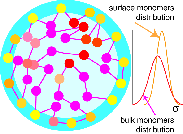
Figure 1: (Color online) Illustration of the model. Monomers are connected by covalent bonds, and monomer type is presented by the shade. Surface is enriched with hydrophilic monomers, such that the distribution of surface monomers $f(\sigma)$ is shifted compared with the bare distribution $p(\sigma)$.

Polymer chain with Hamiltonian (1), with quenched sequence and in the statistical equilibrium in terms of conformation, will exhibit some preference of hydrophilic monomers towards the surface - as long as $\Gamma>0$. The way to characterize this quantitatively is to address the statistics of $\sigma$ values for surface exposed monomers. Namely, we will be interested in distribution $f\left(\sigma\right)$ of surface monomers. We expect this distribution to be different from the bare distribution of all monomers $p\left(\sigma\right)$. Qualitatively, this is illustrated in the inset of Fig. 1.

Of course, the effect of surface exposure to the solvent depends on the sequence. In general, hydrophilic effect adds frustration to the system. Indeed, placing a certain monomer on the surface necessitates placing its sequence neighbors close to the surface, while their identity, or their $\sigma$-values, might imply energetic preference for the interior region of the globule. To address this delicate sequence dependence, we will look at designed sequences.

II.2 Sequence design

Random sequence can be generated by a suitable Poisson process, i.e., by the probability distribution

$$P_{{\rm seq}}^{\left(0\right)}=\prod_{i=1}^{N}p\left(\sigma_{i}\right)\ .$$ (3)

By sequence design, we want to bias the sequence probabilities in a controlled fashion. This can be done in the following way.

The sequence design procedure starts from the choice of the target conformation which we will denote ${\star}$. In our consideration here, ${\star}$ might be any compact conformation, in other words, we ignore the difference of designability for possible target conformations Li et al. (1996) - simply because designability and surface exposure are two independent effects and we do not want to further complicate our work by accounting for designability. There is no doubt that designability along with surface effects must be incorporated into the complete theory. Given a target conformation ${\star}$, we will consider a statistical Gibbs ensemble in which conformation $\{\mathbf{r}_{i}\}={\star}$ is quenched, while the sequence $\{\sigma_{i}\}$ is annealed and comes to thermodynamic equilibrium at the design temperature $T_{d}$, which is not necessarily equal to the real temperature $T$. More specifically, we use the canonical sequence design scheme Pande et al. (1997), in the sense that it is generated by the canonical ensemble of annealed sequences. This results in the following probability distribution of sequences:

$$P_{{\rm seq}}^{\star}=P_{{\rm seq}}^{\left(0\right)}\frac{\exp\left[-H^{d}\left({\rm seq},{\star}\right)/T_{d}\right]}{\sum_{{\rm seq}^{\prime}}P_{{\rm seq}^{\prime}}^{\left(0\right)}\exp\left[-H^{d}\left({\rm seq}^{\prime},{\star}\right)/T_{d}\right]}\ ,$$ (4)

where the denominator ensures normalization. Of course, this is just the scheme, the real features of the ensemble of designed sequences are controlled by the design Hamiltonian, $H^{d}\left({\rm seq},{\star}\right)$. It might be the same Hamiltonian as (1), but this is not at all necessary. Moreover, it is useful to explore the more general situation in which $H^{d}\neq H$. We will use design Hamiltonian of the same functional form as (1), but with the different parameters $\delta\!B^{d}$, and $\Gamma^{d}$ ($\overline{B^{d}}$, although formally included for symmetry, does not play any role in sequence design, because this term in energy is sequence-independent):

$$H^{d}\left({\rm seq},{\star}\right)=\sum_{i<j}^{N}\left(\overline{B^{d}}-\delta\!B^{d}\sigma_{i}\sigma_{j}\right)\Delta_{ij}-\Gamma^{d}\sum_{i\in G^{\star}}^{K}\sigma_{i}\ .$$ (5)

From this point of view, $T_{d}$ is just a parameter which controls the quality of design: when $T_{d}\to\infty$, ensemble of designed sequences is essentially the same as random, while at lower $T_{d}$ designed sequences are statistically strongly biased by optimization the design energy.

We work on artificial model proteins design. In vivo De Novo design of globular protein has long been successfully carried out (see, for example Reagan and Degrado (1989) for a four-helix protein design from first-principle). The off-lattice model sequence design works (Amatori et al. (2005, 2006)) on a 60-residue SH3 protein domain showed that the folding quality of designed sequences vary for this small protein.

II.3 High $T_{d}$ expansion of the sequence-averaged target state energy and Random Energy Model

First let us look at the energy of target conformation ${\star}$, averaged over the ensemble of designed sequences:

$$\langle E_{{\star}}\left({\rm seq}\right)\rangle=\sum_{{\rm seq}}P_{{\rm seq}}^{\star}H\left({\rm seq},{\star}\right)\ .$$ (6)

As in Pande et al. (1997), we can evaluate this to the lowest order in high $T_{d}$ expansion:

$$\langle E_{\star}\left({\rm seq}\right)\rangle = \langle H\rangle+\frac{1}{T_{d}}\left(\langle H^{d}H\rangle-\langle H^{d}\rangle\langle H\rangle\right)$$ (7)

$$= N\overline{B}-\frac{1}{T_{d}}\left(N\delta\!B\delta\!B^{d}+K\Gamma\Gamma^{d}\right)\ .$$

We see that sequence design, on average, leads to the lowering of the target state energy. The only novelty, albeit quite trivial, compared at the volume approximation Pande et al. (1997), is that both contact energy and surface energy terms contribute to the target energy decrease.

A’priori, one could think that the design lowers not only the target state energy, but also energies of some other states - particularly, those similar to the target state. It is well known, however, that because of the geometry of compact conformations there are not many sufficiently similar compact conformations and, therefore, the statistics of energies of other conformations, to a good approximation, remains unaffected by the design (see Pande et al. (2000) for further more detailed discussion of this point). This approximation is equivalent to REM. We will work within this REM approximation.

III Monomer distributions inside and on the surface

III.1 Design by solvation

As stated above, our major goal is to address surface effects in terms of the distribution of $\sigma$ values among surface monomers. With the designed sequences, we can first ask - what is the distribution of surface monomers $p^{\star}(\sigma)$ just in the design state, when conformation is frozen? This is of course fundamentally simple question, because the statistical mechanics of sequences at quenched conformation is not frustrated Pande et al. (2000). Basically, what one has to do is to take probability distribution of sequences (4) and to integrate out all spin variables $\{\sigma_{i}\}$ except surface monomers, i.e., all $i$ except those belonging to the target conformation surface set $G^{\star}$.

As a warm-up, let us perform this procedure for the simple yet important special case of design Hamiltonian, in which we set $\delta\!B^{d}=0$. In this case, design affects only surface monomers. The probability distribution of sequences is tremendously simplified, it can be factorized

$$P_{{\rm seq}}^{\star} = P_{{\rm seq}}^{\left(0\right)}\frac{\exp\left[\left(\Gamma^{d}/T_{d}\right)\sum_{i\in G^{\star}}^{K}\sigma_{i}\right]}{\sum_{{\rm seq}^{\prime}}P_{{\rm seq}^{\prime}}^{\left(0\right)}\exp\left[\left(\Gamma^{d}/T_{d}\right)\sum_{i\in G^{\star}}^{K}\sigma_{i}^{\prime}\right]}$$ (8)

$$= \prod_{j\notin G^{\star}}p(\sigma_{j})\prod_{i\in G^{\star}}p^{\star}(\sigma_{i})\ ,$$

which means that the ensemble of monomers in the bulk of the globule remains unaffected, distributed as $p(\sigma)$, while every surface monomer, independently of others, is distributed as

$$p^{\star}\left(\sigma\right)=cp\left(\sigma\right)\exp\left(\Gamma^{d}\sigma/T_{d}\right)\ ,$$ (9)

where $c$ is the normalization factor, $c=1/\int p\left(\sigma^{\prime}\right)\exp\left(\Gamma^{d}\sigma^{\prime}/T_{d}\right)d\sigma^{\prime}$. Thus, for all monomers, including $N-K$ monomers that were in the bulk during the design process, and $K$ monomers that were on the surface, the overall distribution of $\sigma$ reads

$$p_{\rm tot}(\sigma) = \frac{(N-K)p(\sigma)+Kp^{\star}(\sigma)}{N}$$ (10)

$$= p(\sigma)+\frac{K}{N}\left[p^{\star}(\sigma)-p(\sigma)\right]\ .$$

This result, Eq. (9), indicates that even this simplified design procedure, with $\delta\!B^{d}=0$, favors the hydrophilic monomers on the surface, because for hydrophilic monomers with $\sigma>0$, we have $p^{\star}\left(\sigma\right)>p\left(\sigma\right)$. Compared with the bare monomer distribution $p\left(\sigma\right)$, hydrophilic monomers have larger probability to appear on the surface of target conformation.

The simplified $\delta\!B^{d}=0$ design scheme is reminiscent of the method used in Khokhlov and Khalatur (1999, 2004), in which all the surface monomers of target conformation ($G^{\star}$ in our notation) are made hydrophilic while all the monomers inside the globule are hydrophobic. In our more general consideration, it is just more probable but not necessary for the surface exposed monomers to become hydrophilic during the design. The model of the works Geissler et al. (2004) corresponds to the $T_{d}\to 0$ limit of our theory.

III.2 Surface monomer distribution in the ground state

Let us continue examination of the simplified design scheme, with $\delta\!B^{d}=0$, when only surface energy biases the choice of sequences (design by solvation). Our goal now is to find the surface energy correction terms of the ground state energy and, as the major step in this direction, we need to consider the surface monomer distribution $f(\sigma)$ in the ground state. One should realize that in the ground state, the set of surface exposed monomers may or may not be similar to the set of monomers exposed to the surface during the design; in other words, $f(\sigma)$ might be similar to $p^{\star}(\sigma)$, or might be quite different from it. Therefore, there are two contributions to the surface energy, one due to the monomers exposed to the surface, and the other due to the fact that selection of surface monomers affects the monomer composition left inside the globule. To express this quantitatively, we write for the arbitrary state the equation similar to (10)

$$p_{\rm tot}(\sigma)=p_{\rm in}(\sigma)+\frac{K}{N}\left[f(\sigma)-p_{\rm in}(\sigma)\right]\ ,$$ (11)

where $p_{\rm in}(\sigma)$ is the distribution of monomers left inside. Comparing equation (10) and (11), we find

$$p_{\rm in}(\sigma)\simeq p(\sigma)+\frac{K}{N}\left[p^{\star}(\sigma)-f(\sigma)\right]\ .$$ (12)

As everywhere, we neglect here the terms ${\cal O}\left((K/N)^{2}\right)$. Thus, we directly see already here how the deviation of the state from the target state comes into play.

To compute $f(\sigma)$ for the ground state, we adapt for designed sequences the procedure which was developed in the work Geissler et al. (2004) for random sequence solvation. To make our work self-contained, we briefly outline major steps.

We begin by constructing a separate REM, called sub-REM, for each possible choice of surface monomers, $G$. Indeed, for each $G$ there are still many conformations available. The number of such conformations is naturally written in the form $M_{G}=e^{Ns-K\omega_{G}}$, where $s$ is conformational entropy per monomer in volume approximation, and $\omega_{G}$ is entropy loss due to confinement of some monomers on the surface. Although $M_{G}$ is much smaller than the total number of conformations, $M=e^{sN}$, but the entropy loss caused by fixation of $G$ monomers on the surface is only a surface effect ${\cal O}(K)$. Following Geissler et al. (2004), we adopt a bold approximation that $\omega_{G}=\overline{\omega}$ is independent on $G$; in this approximation, counting all states shows that ${\overline{\omega}}=\ln\left(Ne/K\right)$.

For each sub-REM, energies of all $M_{G}$ states are random in the sense that they depend on random sequence realization, and it is reasonable to assume Geissler et al. (2004) that these energies are independent Gaussian variables, because each energy, according to formula (1), has of order $N$ mutually statistically independent bulk contributions and of order $K$ independent surface contributions. To write down the resulting Gaussian distribution, we should determine corresponding mean and variance. The mean is found by averaging the bulk terms $\left(\overline{B}-\delta\!B\sigma_{i}\sigma_{j}\right)$ over the distribution $p_{\rm in}(\sigma)$ plus averaging the surface terms $-\Gamma\sigma_{i}$ over the distribution $f(\sigma)$, and the variance is similarly found by averaging the second moment. This results finally in the following Gaussian distribution of random energy:

$$w_{G}\left(E\right)\propto\exp\left[-\frac{\left[E-\left(N\overline{B}-K\Gamma\gamma_{G}\right)\right]^{2}}{2N\delta\!B^{2}+2K\delta\!B^{2}\beta_{G}}\right]\ ,$$ (13)

where

$$\gamma_{G} = \int\sigma f\left(\sigma\right)d\sigma\ ,$$

$$\beta_{G} = 2\int\sigma^{2}\left[p^{\star}\left(\sigma\right)-f\left(\sigma\right)\right]d\sigma\ .$$ (14)

Notice that dependence on the surface monomer group $G$ is only through the surface monomer distribution, and that the dependence on design is due to the $p^{\star}(\sigma)$.

Every sub-REM has a certain ground state energy $E_{g}(G)=E_{g}\{f(\sigma)\}$, which is just the lowest of $M_{G}$ random energies drawn independently from the distribution (13). Energy $E_{g}\{f(\sigma)\}$ is still a random variable, its probability distribution can be found from the so-called extreme value statistics Bouchaud and Mezard (1997) (see also Appendix A):

$${\cal W}_{G}\left(E\right)=\frac{1}{T_{\rm fr}}\exp\left[\frac{\delta\!E_{g}}{T_{\rm fr}}-\exp\left[\frac{\delta\!E_{g}}{T_{\rm fr}}\right]\right]\ ,$$ (15)

where $T_{\rm fr}=\delta\!B/\sqrt{2s}$ and $\delta\!E_{g}=E-E_{g}^{\rm typ}\{f(\sigma)\}$ is the deviation of ground state energy from its most probable (typical) value, which includes both volume and surface contributions:

$$E_{g}^{\rm typ}\{f(\sigma)\} = N\left(\overline{B}-2sT_{\rm fr}\right)$$ (16)

$$+ K\left(\overline{\omega}T_{\rm fr}-\Gamma\gamma_{G}+sT_{\rm fr}\beta_{G}\right)\ .$$

Notice that the only dependence of probability distribution ${\cal W}_{G}$ on the surface monomers $G$ is hidden in $\gamma_{G}$ and $\beta_{G}$ inside the most probable energy $E_{g}^{\rm typ}\{f(\sigma)\}$, and the dependence on design is also there inside $\beta_{G}$ (see formula (14). We also mention that $T_{\rm fr}=\delta\!B/\sqrt{2s}$ appearing here as a parameter of the ground state distribution happens to have its physical meaning - it is volume approximated freezing temperature of the random sequence polymer Geissler et al. (2004).

The probability to get ground state energy anywhere below its typical most probable value (16) is exponentially small. However, we try exponentially many times - namely, we have to choose the lowest among $e^{K{\overline{\omega}}}=(Ne/K)^{K}$ sub-REM ground states. Therefore, we have a good chance to find some particular sub-group $G$ with energy noticeably below typical value (16). Essentially, what we have to do now is to resort second time to the extreme value statistics and find the expectation value of the lowest among the sub-REM ground states. It is convenient to perform this operation in a slightly different, but equivalent form. Namely, we note that the low energy tail of the ground state probability distribution, (15), is exponential, and, therefore, it looks effectively like Boltzmann distribution, with $T_{\rm fr}$ playing the role of temperature.

It is useful to note here that treating the tail of the distribution (15) as effective Boltzmann distribution with temperature $T_{\rm fr}$ is reminiscent and essentially equivalent to the consideration given in the book Finkelstein and Ptitsyn (2002) and explaining the origin of phenomenologically discovered quasi-Boltzmann distribution over the ensemble of evolutionary selected proteins.

Returning to our argument, finding lowest among the $E_{g}^{\rm typ}$ of the sub-REMs is equivalent to minimizing the effective “free energy”, in which the effective entropy is given by the number of ways to choose $K$ monomers with distribution $f(\sigma)$ from $N$ monomers with distribution $p_{\rm tot}(\sigma)$:

$$s\{f(\sigma)\}=-\int p_{\rm tot}(\sigma)\left[\phi\ln\phi+\left(1-\phi\right)\ln\left(1-\phi\right)\right]d\sigma\ ,$$ (17)

where $\phi(\sigma)=Kf(\sigma)/Np_{\rm tot}(\sigma)$ has the meaning of the fraction of monomers with type $\sigma$ that are exposed to the surface. Including this effective entropy, we have now the effective “free energy”

$$E_{g}^{\rm typ}\{f(\sigma)\}-T_{\rm fr}Ns\{f(\sigma)\}\ .$$ (18)

We minimize this with respect to $f(\sigma)$, subject to normalization condition $\int f(\sigma)d\sigma=1$ and obtain

$$f(\sigma)=\frac{N}{K}\frac{p_{\rm tot}(\sigma)}{1+\Lambda e^{\eta_{\rm fr}(\sigma)}}\ ,$$ (19)

where $\eta_{\rm fr}(\sigma)=2s\sigma^{2}-\left(\Gamma/T_{\rm fr}\right)\sigma$, and $\Lambda$ is the Lagrange multiplier which has to be determined from the normalization condition $\int f(\sigma)d\sigma=1$. Comparing this with the paper Geissler et al. (2004), we see that the only role of design in this case is the modification of monomer distribution: instead of bare distribution $p(\sigma)$, we have now the modified one $p_{\rm tot}(\sigma)$. Let us see what are the consequence of this replacement.

Let us concentrate on the regime without the depletion effect, when $\phi(\sigma)\ll 1$ at all values of $\sigma$. This means that for any monomer type, only a small fraction of it is solvated to the surface region. Under such assumption, $f(\sigma)$ can be approximated as

$$f(\sigma)\propto e^{-\eta_{\rm fr}(\sigma)}\left[1+\frac{K}{N}\left(c\exp\left(\frac{\Gamma^{d}}{T_{d}}\sigma\right)-1\right)\right]p(\sigma)\ ,$$ (20)

where we dropped for simplicity the $\sigma$-independent normalization factor. To gain some insight, let us look at $f(\sigma)$ for a couple of simple examples of bare monomer probability distributions. Since real distribution involves a large number ($20$) of monomer species, we examine two limits of two monomer species and of continuous Gaussian distribution.

III.2.1 Example: bimodal distribution

In the simplest black-and-white model Dill and the others (1995) two types of monomers, one hydrophilic and one hydrophobic, appear with same probability:

$$p\left(\sigma\right)=\frac{1}{2}\left[\delta\!\left(\sigma+1\right)+\delta\left(\sigma-1\right)\right]\ .$$ (21)

Simple calculation shows that

$$f\left(\sigma\right) \propto \delta\left(\sigma+1\right)e^{-\Gamma/T_{\rm fr}}\left[1-\frac{K}{N}\tanh\left(\frac{\Gamma^{d}}{T_{d}}\right)\right]+$$ (22)

$$\delta\left(\sigma-1\right)e^{\Gamma/T_{\rm fr}}\left[1+\frac{K}{N}\tanh\left(\frac{\Gamma^{d}}{T_{d}}\right)\right]\ .$$

We see that there are two effects bringing hydrophilic monomers to the surface, that is, increasing $f(+1)$ on the expense of decreasing $f(-1)$. First effect is due to $\Gamma$ and is measured by the ratio $\Gamma/T_{\rm fr}$. This effect is present in random heteropolymer, has nothing to do with design, and is simply energetic: since it is more favorable for the $\sigma>0$ monomers to be on the surface, so the surface gets enriched with such monomers. The second effect is entirely due to design and it is governed by the design parameters $\Gamma^{d}/T_{d}$. This effect is washed way at large design temperature and it saturates at small $T_{d}$. Notice that this design effect is only a surface effect, its maximal possible role is proportional to $K/N$. This is because the best one can do with this type of design is to shift the monomeric composition by the amount about $K/N$.

III.2.2 Example: Gaussian distribution

The opposite limit is presented by

$$p\left(\sigma\right)=\frac{1}{\sqrt{2\pi}}\exp\left(-\frac{\sigma^{2}}{2}\right)\ .$$ (23)

The corresponding surface monomer distribution is the following:

$$f\left(\sigma\right) \propto \left[1+\frac{K}{N}\left[\exp\left(\frac{\Gamma^{d}\sigma}{T_{d}}-\frac{1}{2}\left(\frac{\Gamma^{d}}{T_{d}}\right)^{2}\right)-1\right]\right]$$ (24)

$$\times\exp\left(-\frac{1+4s}{2}\sigma^{2}+\frac{\Gamma}{T_{\rm fr}}\sigma\right)\ .$$

In Fig. 2, we made a plot of an example of $f(\sigma)$ as a function of $\sigma$ for the Gaussian case. For comparison, random sequence solvation ($T_{d}\to\infty$) is also included. It can be seen that design enriches surface with hydrophilic monomers such that the distribution is shifted toward hydrophilic region compared to no design case, which by itself is already a shift relative to the bare distribution $p(\sigma)$.

Figure 2: (Color online). A comparison of original distribution and surface monomer distribution with design, together with the case of without design. Design favors the monomers with hydrophilic type.

III.3 Sequence design by both solvation and monomer contacts: mean field approximation

In the preceding section, we considered sequences designed by the effect of preferential solvation of certain monomer types under the chain preparation conditions. This corresponds to having only the second term in the design Hamiltonian (5) , or having $\delta\!B^{d}=0$. By contrast, sequence design by monomer-monomer contacts, i.e. the limit of $\Gamma^{d}=0$ and $\delta\!B^{d}\neq 0$ was considered in the literature before (see, e.g., review article Pande et al. (2000) and references therein).

In this section, we consider the general case, when both volume and surface terms of the design Hamiltonian (5) are present. To make the argument, we resort to the mean-field approximation for the design system. That means, we consider design by an effective field which couples to the variables $\sigma$ and acts differently on surface and bulk monomers. Since design Hamiltonian (5) is quadratic in $\sigma$, the said “design field” is proportional to $\overline{\sigma}$ - an average value of $\sigma$ defined self-consistently. It is then easy to realize that this field vanishes in the bulk, because in our model design does not affect overall composition of the chain, and, therefore, $\overline{\sigma}_{\rm bulk}=0$. Therefore, the mean field approximated design Hamiltonian reads

$$H^{d}_{\rm mean\ field}\simeq-\left(\delta\!B^{d}z\overline{\sigma}_{\rm surf}+\Gamma^{d}\right)\sum_{j\in G^{\star}}^{K}\sigma_{j}\ .$$ (25)

Here, $\overline{\sigma}_{\rm surf}$ is the average $\sigma$ of surface monomers (that is, of monomers which happen to be on the surface during the design process) and $z$ is the coordination number (the number of neighbors) for surface monomers.

Within the mean field approximation, the probability distribution of designed sequences (4) gets factorized into independent distributions of all monomers, just like in the $\delta\!B^{d}=0$ case. Accordingly, we obtain the distribution of surface monomers, similar to Eq. (9):

$$p^{\star}(\sigma)\propto p(\sigma)\exp\left[\frac{\delta\!B^{d}z\overline{\sigma}_{\rm surf}+\Gamma^{d}}{T_{d}}\sigma\right]\ ,$$ (26)

where we dropped for brevity the $\sigma$-independent normalization factor. Now, the value of $\overline{\sigma}_{\rm surf}$ must be determined from the self-consistency condition

$$\overline{\sigma}_{\rm surf} = \int\sigma p^{\star}(\sigma)d\sigma$$ (27)

$$= \frac{\int\sigma p(\sigma)\exp\left[\frac{\delta\!B^{d}z\overline{\sigma}_{\rm surf}+\Gamma^{d}}{T_{d}}\sigma\right]d\sigma}{\int p(\sigma)\exp\left[\frac{\delta\!B^{d}z\overline{\sigma}_{\rm surf}+\Gamma^{d}}{T_{d}}\sigma\right]d\sigma}\ .$$

To gain an insight into the properties of the latter equation, it is useful to consider the examples of bimodal and Gaussian distributions for $p(\sigma)$. We do that a few lines below, in section III.4, but here we notice that once $\overline{\sigma}_{\rm surf}$ is determined, the rest of the analysis follows automatically along the lines of our previous consideration in the section III.2. Indeed, all we needed to know to implement the result (19) is the overall monomer distribution $p_{\rm tot}(\sigma)$, which is known as soon as $p^{\star}(\sigma)$ is determined (see Eq. (10)). Therefore, we can directly use our results Eqs (20), (22), (24) with the replacement $\Gamma^{d}\to\Gamma^{d}+\delta\!B^{d}z\overline{\sigma}_{\rm surf}\equiv\Gamma^{\prime d}$.

With that in mind, let us return briefly to the determination of $\overline{\sigma}_{\rm surf}$.

III.4 Implementing the self-consistency condition

III.4.1 Example: bimodal distribution

For bimodal $p(\sigma)$, Eq. (27) becomes

$$\overline{\sigma}_{\rm surf}=\tanh\left[\frac{\delta\!B^{d}z\overline{\sigma}_{\rm surf}+\Gamma^{d}}{T_{d}}\right]\ .$$ (28)

At $\Gamma^{d}=0$, this equation has non-trivial non-vanishing solutions only if $\delta\!B^{d}z/T_{d}>1$, in which case there are automatically two solutions of the opposite sign. That means, the non-zero $\overline{\sigma}_{\rm surf}$ in this case results only from the spontaneous symmetry breaking, because without $\Gamma^{d}$ the system has no preference for hydrophobic or hydrophilic monomers dominating the surface. The non-zero $\Gamma^{d}>0$ breaks this symmetry and yields always one and only one positive solution for $\overline{\sigma}_{\rm surf}$ (and possibly two negative ones which we ignore because they have higher free energy).

In this bimodal case, we have $\overline{\sigma}_{\rm surf}<1$, which means that in the replacement $\Gamma^{d}\to\Gamma^{\prime d}$, the solvation term $\Gamma^{d}$ dominates if $\Gamma^{d}>\delta\!B^{d}z$.

III.4.2 Example: Gaussian distribution

For Gaussian $p(\sigma)$, Eq. (27) is easily explicitly resolved:

$$\overline{\sigma}_{\rm surf}=\frac{\Gamma^{d}/T_{d}}{1-z\delta\!B^{d}/T_{d}}\ .$$ (29)

This is usually very close to $\Gamma^{d}/T_{d}$, because (see next section IV) in most interesting regime close to the triple point of the phase diagram, the denominator is dominated by the unity.

IV Free energy and phase diagram of designed polymers

IV.1 Preliminary remarks

In this section, we will consider the possible phases of the heteropolymer whose sequence is designed as discussed above. Similar problem in volume approximation is well known in the literature (see, e.g., review Pande et al. (2000) and references therein). Specifically, we will consider three phases and the transitions between them. We will summarize the relations between phases in terms of the phase diagram, Fig. 3, in variables $T_{d}$ and $T$, which describe, respectively, the ensemble of sequences and the ensemble of conformations for any given sequence. The relevant phases in the diagram are named, respectively, liquid-like globule, glassy globule, and folded globule. We remind to the reader that liquid-like globule is the state where great many conformations contribute to the partition function; glassy globule is dominated by one or a few conformations, but those unrelated to the target conformation $\star$; and folded globule is dominated by the target conformation $\star$. It is fairly obvious and illustrated in Fig. 3, that surface solvation effects do not change the topology of the phase diagram, but does affect the specific positions and shape of the corresponding phase transition lines; these surface-driven changes are the subject of our interest in this section.

The temperatures of the transitions from liquid-like to glass-like and to folded globules are called glass temperature $T_{g}$ and folding temperature $T_{f}$, respectively. Our goal is to analyze the role of surface solvation effects and design on both $T_{g}$ and $T_{f}$. In other words, we want to calculate how surface corrections to $T_{f}$ and $T_{g}$ depend on the design temperature $T_{d}$.

As regards the third phase transition line, that between folded and glassy globule phases, this line must be vertical in phase diagram. Indeed, both folded and glassy globules are zero entropy states, the transition between them cannot be driven by temperature change. On the phase diagram, like in Fig. 3, the corresponding phase boundary must be represented by the line parallel to the temperature axis. This argument does not rely on the volume approximation, and, therefore, remains valid independently of the surface solvation effects. Therefore, this line of phase transition is entirely described by the value of design temperature at which there is the triple point, we call it $T_{d}^{(3)}$. We want to calculate also the surface contribution to this quantity.

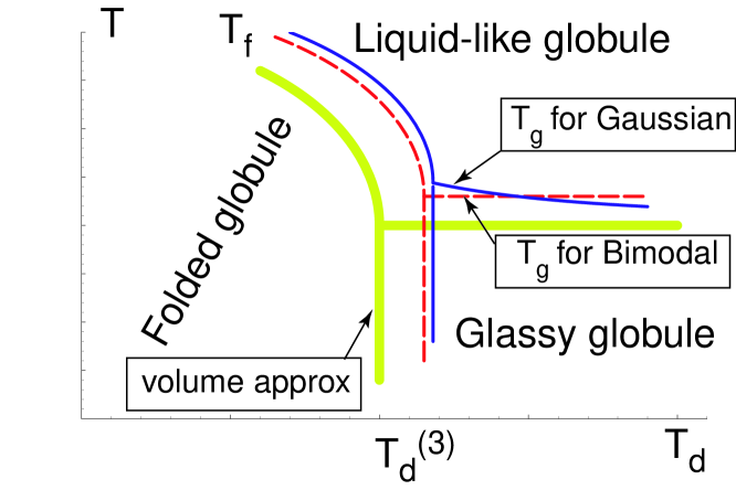
Figure 3: (Color online) Phase diagram of the heteropolymer system. There are three phases: random liquid-like globule, frozen glassy globule and folded globule. Surface term shifts the phase diagram for volume approximation. For bimodal distribution, glass temperature is design independent, while in Gaussian distribution, glass temperature increases for better design condition.

The way we approach the phase diagram is based on the idea that for any frozen globule phase, whether glassy or folded, the free energy coincides with energy, because entropy vanishes given the number of contributing states of order unity. On the other hand, the free energy of the liquid-like globule we can find due to the property of REM that quenched averaged free energy is equal to the annealed average above the glass temperature. Therefore, what we shall do is to compute the annealed average free energy and to find temperature of entropy “catastrophe” - at which entropy vanishes; that is the glass temperature. Of course, our goal is to address surface terms and design terms in this procedure. Following this program, we write the annealed average as a functional of the surface monomer distribution $f(\sigma)$ as

$$F\{f\} = -T\ln\sum_{{\rm conf}}e^{-E/T}$$ (30)

$$\simeq -T\ln\int e^{sN-K\omega_{G}+Ns\{f(\sigma)\}}w_{G}(E)e^{-E/T}dE$$

$$\simeq \overline{F}+F_{\rm surf}\{f\}\ ,$$

where

$$\frac{\overline{F}}{N}=\overline{B}-sT-\frac{\delta\!B^{2}}{2T}$$ (31)

is the bulk contribution to the free energy, and

$$\frac{F_{\rm surf}\{f\}}{K} = \overline{\omega}T-\frac{\delta\!B^{2}}{T}\int\sigma^{2}p^{\star}(\sigma)d\sigma+\frac{N}{K}T\int d\sigma p_{\rm tot}(\sigma)$$ (32)

$$\times\left[\phi\left(\eta(\sigma)-\ln\frac{1-\phi}{\phi}\right)+\ln(1-\phi)\right]$$

is the surface contribution to free energy. In Eq. (32),

$$\eta(\sigma) = \frac{\delta\!B^{2}}{T^{2}}\sigma^{2}-\frac{\Gamma}{T}\sigma\ ,$$

$$p^{\star}\left(\sigma\right) = \frac{p\left(\sigma\right)\exp\left(\frac{\Gamma^{\prime d}}{T_{d}}\sigma\right)}{\int p\left(\sigma\right)\exp\left(\frac{\Gamma^{\prime d}}{T_{d}}\sigma\right)d\sigma}\ .$$ (33)

In deriving the free energy, we have used the saddle point approximation since above glass temperature, free energy is dominated by the saddle point of the partition function.

Optimizing $F_{\rm surf}\{f\}$ yields

$$\phi^{\star}=\frac{1}{1+\Lambda e^{\eta(\sigma)}}=\frac{Kf^{\star}(\sigma)}{Np_{\rm tot}(\sigma)}\ ,$$ (34)

and then optimal value of $F_{\rm surf}\{f\}$ evaluates to

$$\frac{F_{\rm surf}\{f^{\star}\}}{KT}=1+\frac{\int p_{\rm tot}(\sigma)\ln\frac{\Lambda e^{\eta(\sigma)}}{1+\Lambda e^{\eta(\sigma)}}d\sigma}{\int\frac{p_{\rm tot}(\sigma)}{1+\Lambda e^{\eta(\sigma)}}d\sigma}$$

$$-\frac{\delta\!B^{2}}{T^{2}}\int\sigma^{2}p^{\star}(\sigma)d\sigma-\ln\int\frac{\Lambda p_{\rm tot}(\sigma)}{1+\Lambda e^{\eta(\sigma)}}d\sigma\ .$$ (35)

These results are similar to those obtained in the work Geissler et al. (2004), except we have now non-random sequences, as manifested by the dependence on $T_{d}$. In that work Geissler et al. (2004), solvation effect in random sequences was treated as the response of the globule to the surface solvation “field”. The linear response regime is characterized by the statistical independence of disordered parts of surface and volume energies. Saturation regime is characterized by the depletion effect, when preferential solvation of a certain monomer species exhausts these monomers from the globule. For completeness, there is also a narrow range of the so-called weak response regime. Neither weak response nor saturation regimes are present for the black-and-white polymer model, with bimodal distribution of monomer types.

IV.2 No depletion: Glass temperature

Let us first consider the case when solvation doesn’t cause the depletion of any monomer type, that is, $\phi(\sigma)\ll 1$ at every $\sigma$, then

$$\frac{F_{\rm surf}\{f^{\star}\}}{KT}\simeq-\frac{\delta\!B^{2}}{T^{2}}\int\sigma^{2}p^{\star}(\sigma)d\sigma-\ln\int p_{\rm tot}(\sigma)e^{-\eta(\sigma)}d\sigma\ .$$ (36)

First we will discuss how the glass temperature $T_{g}$ is affected by the surface energy, relative to the volume approximated value $T_{\rm fr}=\delta\!B/\sqrt{2s}$. Glass temperature must be determined from by the condition $-\left.\frac{\partial F\{f\}}{\partial T}\right|_{T_{g}}=0$. Since $-\left.\frac{\partial\overline{F}}{\partial T}\right|_{T_{\rm fr}}=0$, we can write (denoting temperature derivatives by prime sign) $\Delta T_{g}\simeq T_{g}-T_{\rm fr}\simeq-\left.\frac{F_{\rm surf}^{\prime}}{\overline{F}^{\prime\prime}}\right|_{T_{\rm fr}}$. Then

$$\frac{\Delta T_{g}}{T_{\rm fr}} \simeq \frac{K}{N}\left[\frac{\Gamma}{2sT_{\rm fr}}\frac{\int\sigma p(\sigma)e^{-\eta_{\rm fr}(\sigma)}d\sigma}{\int p(\sigma)e^{-\eta_{\rm fr}(\sigma)}d\sigma}\right.$$ (37)

$$\left.+\int\sigma^{2}p^{\star}(\sigma)d\sigma-\frac{2\int\sigma^{2}p(\sigma)e^{-\eta_{\rm fr}(\sigma)}d\sigma}{\int p(\sigma)e^{-\eta_{\rm fr}(\sigma)}d\sigma}\right.$$

$$\left.-\frac{1}{2s}\ln\int p(\sigma)e^{-\eta_{\rm fr}(\sigma)}d\sigma\right]\ ,$$

where we have replaced $p_{\rm tot}(\sigma)$ with $p(\sigma)$ because $\Delta T_{g}$ itself is already of order ${\cal O}\left(K/N\right)$, and we neglect any higher order corrections. Design effect is present here through $p^{\star}(\sigma)$.

Relative to no solvation case, the order ${\cal O}(K/N)$ correction to glass temperature is positive; in other words, glass temperature is increased due to the solvation effect, so the surface effect makes ground state more stable.

In the following part, we will further simplify and discuss $\Delta T_{g}$ using the examples of $p(\sigma)$.

IV.2.1 Example: bimodal distribution

For bimodal $p(\sigma)$, $\int\sigma^{2}p^{\star}(\sigma)d\sigma=1$, and design effect doesn’t show up in glass temperature,

$$\Delta T_{g} = \frac{K}{2sN}T_{\rm fr}\left[\frac{\Gamma}{T_{\rm fr}}\tanh\left(\frac{\Gamma}{T_{\rm fr}}\right)-\ln\cosh\left(\frac{\Gamma}{T_{\rm fr}}\right)\right]$$ (38)

$$\simeq \frac{K}{N}\begin{cases}\frac{\Gamma^{2}}{2\sqrt{2s}\delta\!B}&\text{when $\frac{\Gamma}{T_{\rm fr}}\ll 1$}\\ \frac{\ln 2}{(2s)^{3/2}}\delta\!B&\text{when $\frac{\Gamma}{T_{\rm fr}}\gg 1$}\end{cases}\ .$$

When the solvation strength $\Gamma$ is small, $\Gamma/T_{\rm fr}\ll 1$, this corresponds to the statistical independent region, in which surface term and volume term in a heteropolymer globule are roughly statistically independent. In this region, $\Delta T_{g}\propto\Gamma^{2}$.

The region of $\Gamma/T_{\rm fr}\gg 1$ is saturation region. When solvation strength $\Gamma$ is so large, essentially all the surface monomers are of hydrophilic type, as can be clearly seen from surface monomer distribution Eq. (22): when $\Gamma/T_{\rm fr}\gg 1$, surface monomer distribution function is dominated by hydrophilic term $f(+1)$. In this regime, $\Delta T_{g}$ becomes independent of $\Gamma$, because $\Gamma$ is already so large that all surface places are occupied by hydrophilic monomers and further increase of $\Gamma$ cannot change anything.

IV.2.2 Example: Gaussian distribution

For Gaussian $p(\sigma)$, we can write $\int\sigma^{2}p^{\star}(\sigma)d\sigma=\left(\Gamma^{\prime d}/T_{d}\right)^{2}+1\simeq\left(\Gamma^{d}/T_{d}\right)^{2}\left(1+2z\delta\!B^{d}/T_{d}\right)+1\simeq\left(\Gamma^{d}/T_{d}\right)^{2}+1$, where the asymptotic form comes from the fact that $T_{d}/(z\delta\!B^{d})\gg 1$ since we work in the regime of $T_{d}>T_{d}^{(3,0)}=\delta\!B^{d}/\sqrt{2s}$, where $T_{d}^{(3,0)}$ is the triple point in volume approximation. Then we have

$$\Delta T_{g}\simeq\frac{K}{N}T_{\rm fr}\left[\left(\frac{\Gamma^{d}}{T_{d}}\right)^{2}+6s+\frac{\Gamma^{2}}{2\delta\!B^{2}}\right]\ ,$$ (39)

where we also used the fact that $s\ll 1$. As in the work Geissler et al. (2004), system with Gaussian distributed $\sigma$, unlike bimodal one, has the weak response regime at very small $\Gamma$, when $\Gamma/T_{\rm fr}\ll s$; in this regime, surface solvation is insignificant. The region of $\Gamma/T_{\rm fr}\gg\sqrt{24}s$ is the regime where volume and surface disorder are statistically independent, and the result in this region, in terms of dependence on $\Gamma$, is similar to that of the bimodal distribution.

Of course, the major difference from the bimodal example is that in Gaussian case, there is an additional term due to sequence design. That term increases glass temperature, which means design, as usually, makes for a more stable ground state.

IV.3 Triple point

Now let us consider the folded region, and begin with the surface-corrected triple point $T_{d}^{(3)}$; we want to see its change $\Delta T_{d}^{(3)}=T_{d}^{(3)}-T_{d}^{(3,0)}$ relative to $T_{d}^{(3,0)}=\delta\!B^{d}/\sqrt{2s}$ determined in volume approximation. In general, triple point is determined from the condition that glass temperature equals folding temperature, $T_{f}=T_{g}$. Glass temperature, along with its surface corrections, is already known to us, see formula (37) or its simplified versions (38) and (39). The folding temperature $T_{f}$ should be calculated from $\langle E_{\star}({\rm seq})\rangle=F\{f^{\star}\}$. We take averaged ground state energy from formula (7) and we take $F\{f^{\star}\}$ from Eqs. (31) and (35); in the latter (which is the surface part) we must neglect all order ${\cal O}(K/N)$ corrections. The result reads

$$\Delta T_{d}^{(3)} \simeq \frac{K}{N}T_{d}^{(3,0)}\left[\frac{\Gamma\Gamma^{d}}{\delta\!B\delta\!B^{d}}-\int\sigma^{2}p^{\star}(\sigma)d\sigma\right.$$ (40)

$$\left.-\frac{1}{2s}\ln\int p(\sigma)e^{-\eta_{\rm fr}(\sigma)}d\sigma\right]\ .$$

From this formula, it is not even clear whether $\Delta T_{d}^{(3)}$ is positive or negative. As with other cumbersome results, let us look at the specific examples of $p(\sigma)$.

IV.3.1 Example: bimodal distribution

For bimodal distribution $p(\sigma)$, we have

$$\Delta T_{d}^{(3)}\simeq\frac{K}{N}T_{d}^{(3,0)}\left[\frac{\Gamma\Gamma^{d}}{\delta\!B\delta\!B^{d}}-\frac{1}{2s}\ln\cosh\left(\frac{\Gamma}{T_{\rm fr}}\right)\right]$$ (41)

$$\simeq \begin{cases}\frac{K}{N}T_{d}^{(3,0)}\frac{\Gamma}{\delta\!B}\left(\frac{\Gamma^{d}}{\delta\!B^{d}}-\frac{\Gamma}{2\delta\!B}\right)&\text{when $\frac{\Gamma}{T_{\rm fr}}\ll 1$}\\ \frac{K}{N}T_{d}^{(3,0)}\frac{\Gamma}{\delta\!B}\left(\frac{\Gamma^{d}}{\delta\!B^{d}}-\frac{1}{\sqrt{2s}}\right)&\text{when $\frac{\Gamma}{T_{\rm fr}}\gg 1$}\end{cases}\ .$$

We see that the design effect increases $\Delta T_{d}^{(3)}$, pushes triple point to the right on the phase diagram Fig. 3, while the solvation effect acts in the opposite direction. Interestingly, in the statistical independence regime, when $\Gamma/T_{\rm fr}\ll 1$, the sign of $\Delta T_{d}^{(3)}$ is determined by the competition of the design term $\Gamma^{d}/\delta\!B^{d}$ and folding term $\Gamma/\delta\!B$. Specifically, large design solvation strength $\Gamma^{d}/\delta\!B^{d}\gg\Gamma/\delta\!B$ would make $\Delta T_{d}^{(3)}>0$ and in this sense the design makes folded state more stable. From Eq. (38), we already know that glass temperature is independent of $\Gamma$ in saturation region $\Gamma/T_{\rm fr}\gg 1$. Not surprisingly, in this region, the sign of $\Delta T_{d}^{(3)}$ is also independent of $\Gamma$.

IV.3.2 Example: Gaussian distribution

When $p(\sigma)$ is Gaussian, we get

$$\Delta T_{d}^{(3)} \simeq \frac{K}{N}T_{d}^{(3,0)}\left[\frac{\Gamma{\Gamma}^{d}}{\delta\!B\delta\!B^{d}}-\frac{\Gamma^{2}}{2\delta\!B^{2}}-2s\right.$$ (42)

$$\left.-2s\left(\frac{\Gamma^{d}}{\delta\!B^{d}}\right)^{2}(1+2z\sqrt{2s})\right]\ .$$

The interesting and rather unexpected result is that the design effect, when it is very strong, might lead to reduction of $T_{d}^{(3)}$; in other words, it might have an adverse effect on the stability of the folded phase. Inspection of the origin of the negative term $\propto-(\Gamma_{d}/\delta\!B^{d})^{2}$ shows that its origin is due to the fact that very strong solvation effect in design brings in a significant fraction of very strongly solvophilic monomers; even though only small fraction of them subsequently turns out inside the globule in the folded state, they nevertheless make the destabilizing effect on the globule. We emphasize that such danger exists only when solvation effect in design is so strong that not only $\Gamma^{d}/\delta\!B^{d}>\Gamma/\delta\!B$, but $s\Gamma^{d}/\delta\!B^{d}>\Gamma/\delta\!B$. It is unclear if such situation is realistic.

IV.4 Folding temperature

Next let us consider the folding temperature $T_{f}$ away but not far from the triple point. When $T_{d}<T_{d}^{(3)}$, we have

$$\frac{\delta\!B\delta\!B^{d}+\frac{K}{N}\Gamma\Gamma^{d}}{T_{d}}=\left.\left(sT+\frac{\delta\!B^{2}}{2T}+F_{\rm surf}\right)\right|_{T=T_{f}}\ .$$ (43)

In the vicinity of the triple point, when $T_{d}=T_{d}^{(3)}-\Delta T_{d}$, where $\Delta T_{d}\ll\frac{K}{N}T_{d}^{(3)}$, we have $F_{\rm surf}|_{T=T_{f}}\simeq F_{\rm surf}|_{T=T_{g},T_{d}=T_{d}^{(3,0)}}$, or

$$\frac{\delta\!B\delta\!B^{d}}{T_{d}^{(3)}}\frac{\Delta T_{d}}{T_{d}^{(3)}}\simeq sT_{f}+\frac{\delta\!B^{2}}{2T_{f}}-sT_{g}-\frac{\delta\!B^{2}}{2T_{g}}\ ,$$ (44)

which yields upon some algebra

$$T_{f}\simeq T_{g}\left[1+\sqrt{\frac{\delta\!B\delta\!B^{d}}{sT_{d}^{(3)}T_{g}}\left(1-\frac{T_{d}}{T_{d}^{(3)}}\right)}\right]\ .$$ (45)

In Fig. 3, the phase diagram of the system is sketched. In the regime of temperature $T$ below $T_{f}$, the designed sequences will thermodynamically stable when folded to the target state. In the regime of $T_{d}>T_{d}^{(3)}$, sequences obtained will be either in frozen glassy state or in random liquid-like globule.

IV.5 Depletion effect

In preceding sections, we assumed no depletion effect. Here we will see what happens if there is depletion. Depletion of monomers may happen for Gaussian $p(\sigma)$, while in bimodal case, there is no depletion since the number of monomers for each monomer type is abundant. When depletion occurs, $\phi=1$ for $\sigma\geq\sigma_{m}$, and $\phi=0$ for $\sigma<\sigma_{m}$, and this leads to

$$\int_{\sigma_{m}}^{\infty}p_{\rm tot}(\sigma)d\sigma=K/N\ .$$ (46)

The integration result is

$$\underbrace{{\rm erfc}\left(\frac{\sigma_{m}-\frac{\Gamma^{\prime d}}{T_{d}}}{\sqrt{2}}\right)-{\rm erfc}\left(\frac{\sigma_{m}}{\sqrt{2}}\right)}_{>0}-2=-\frac{N}{K}{\rm erfc}\left(\frac{\sigma_{m}}{\sqrt{2}}\right)\ .$$ (47)

For the case of no design, $\Gamma^{\prime d}=0$,

$${\rm erfc}\left(\frac{\sigma_{m}^{0}}{\sqrt{2}}\right)=\frac{2K}{N}\ .$$ (48)

Therefore, we have ${\rm erfc}\left(\sigma_{m}/\sqrt{2}\right)<{\rm erfc}\left(\sigma_{m}^{0}/\sqrt{2}\right)$, and this gives $\sigma_{m}>\sigma_{m}^{0}$, so with design, the surface monomers are more hydrophilic than without design. This makes physical sense and this is also consistent with no depletion case $\phi\ll 1$, in which design favors the hydrophilic monomers on the surface.

V Sequence space entropy

Sequence design, when it is realized computationally, or if it could be realized experimentally, helps finding sequences with particularly low ground state energy. But of course there is a limit - there is always a sequence whose ground state energy is the lowest among all sequences, and, therefore, no design can possibly produce any sequence with lower energy. More generally and more practically, the lower ground state energy we want to obtain, the fewer sequences exist which can meet our demand. One may want to know how many sequences are there to choose from with any given ground state energy. Design paradigm provides the general method to solve such problem. Indeed, we can compute the sequence space entropy (which is just the logarithm of the number of relevant sequences) as a function of $T_{d}$ and as we also know the average ground state energy as a function of $T_{d}$, we can determine the number of sequences as depends on their ground state energy. This procedure in volume approximation is described in the work Pande et al. (2000). Here we want to consider how it is affected by the surface solvation effect.

In principle, sequence space entropy depends quite strongly on the target state fold here denoted as $\star$, this dependence is called designability of the fold (see, for example, recent work on this subject Wong and Frishman (2006)). Here, we will neglect this fact. This is not because designability is unimportant - it is very important indeed, but our goal is to look at the role of sequence solvation effect, so to make this task manageable, we have to sacrifice the designability issue as a zeroth approximation.

To find sequence space entropy, we consider sequence space free energy $-T_{d}\ln Z$, where $Z=\sum_{{\rm seq}}\exp\left[-H^{d}({\rm seq},{\star})/T_{d}\right]$. Note that design is to a certain conformation $\star$, so in the partition function here, the summation runs over sequences. Sequence space entropy per monomer $s_{\rm seq}$ can then be found using high $T_{d}$ expansion just in the same way as the calculation of $\langle E_{\star}(seq)\rangle$, formula (7). The result is given by

$$s_{\rm seq}=-\frac{\partial\left(-T_{d}\ln Z\right)}{\partial T_{d}}\simeq\ln q-\frac{\delta\!{B^{d}}^{2}+\frac{K}{N}{\Gamma^{d}}^{2}}{2T_{d}^{2}}\ ,$$ (49)

where $q$ is the effective number of ‘letters in the alphabet’ determined from the total number of possible sequences of length $N$: ${\cal N}_{\rm seq}=q^{N}$. It is not difficult to show that $q=-\sum_{\sigma}p(\sigma)\ln p(\sigma)$ (see Eq. (3); $q\approx 18$ for real proteins).

The number of sequences is maximal if we impose no constraints on the quality of design, which means sequence entropy has to be maximal when $T_{d}$ is at the triple point. Therefore, we can compute $s_{{\rm seq}}^{\rm max}$ using formula (49) at $T_{d}=T_{d}^{(3)}$. The result reads:

$$s_{{\rm seq}}^{\rm max}\simeq\ln q-s\left[1-\frac{2\Delta T_{d}^{(3)}}{T_{d}^{(3,0)}}+\frac{K{\Gamma^{d}}^{2}}{N\delta{\!B^{d}}^{2}}\right]\ ,$$ (50)

where the ratio $\Delta T_{d}^{(3)}/T_{d}^{(3,0)}$ should be taken from Eq. (40) or from the simplified versions of it (41) or (42).

First, in the volume approximation, when there is no surface term, we have $s_{{\rm seq}}^{\rm max}=\ln q-s$. This result is a very natural consequence of our neglect of the difference in designabilities between different folds. Indeed, volume approximation of $s_{{\rm seq}}^{\rm max}$ indicates that the number of sequences that can be designed for a given conformation $\star$ is $e^{Ns_{{\rm seq}}^{\rm max}}={\cal N}_{{\rm seq}}/{\cal N}_{{\rm conf}}$, which means that all ${\cal N}_{{\rm seq}}=q^{N}$ sequences are equally distributed between ${\cal N}_{\rm conf}=e^{sN}$ conformations. This is because the fraction of sequences with ground state energy above $\langle E_{\star}(seq)\rangle$ (7) is extremely small, see appendix A.1, so practically all sequences have their ground state energy around $\langle E_{\star}(seq)\rangle$.

Second, we look at the role of surface effect. For simplicity, we restrict consideration to the most typical regime of statistical independence between surface and bulk contributions. For both bimodal distribution and Gaussian distribution, plugging $\Delta T_{d}^{(3)}$ into Eq. (50), we get the following simple result:

$$s_{\rm seq}^{\rm max}=\ln q-s-\frac{sK}{N}\left[\frac{\Gamma}{\delta\!B}-\frac{\Gamma^{d}}{\delta\!B^{d}}\right]^{2}\ .$$ (51)

This tells us that the surface solvation effect reduces the number of sequences, $s_{\rm seq}^{\rm max}<\ln q-s$. This happens because some of the sequences, with inadequate supply of hydrophilic monomers, have their ground state energies above $\langle E_{\star}(seq)\rangle$ when we look at them carefully enough to notice their surface energy. Accordingly, the fraction of sequences with ground state at $\star$ is below its ‘fair’ share of $e^{(\ln q-s)N}$ and even maximal sequence space entropy falls short of its volume approximated value $\ln q-s$. Only very careful design, at which $\Gamma^{d}/\delta\!B^{d}=\Gamma/\delta\!B$, would be able to provide the ensemble of sequences adequate to their solvation conditions, in which case the solvation effect does not increase energy and does not rule any sequences out of the competition. Notice that the condition $\Gamma^{d}/\delta\!B^{d}=\Gamma/\delta\!B$ does not involve design temperature, it specifies only the balance of solvation and bulk heteropolymeric effects.

Let us now look at the situation differently, namely, let us write down the folding temperature $T_{f}$ in terms of $s_{\rm seq}$ instead of $T_{d}$. Indeed, $T_{d}$ is a purely technical concept which may or may not directly correspond to the experimental reality; for instance, design can be controlled by some analog of solvent quality instead of temperature. At the same time, sequence entropy is a very clear quantity, it is the number of sequences whose ground state stability corresponds to the temperature $T_{f}$. Simple algebra shows that

$$T_{f}=T_{g}\left[1+\sqrt{\frac{\delta\!B\delta\!B^{d}}{sT_{g}T_{d}^{(3)}}\left(1-\sqrt{\frac{\ln q-s_{\rm seq}^{\rm max}}{\ln q-s_{\rm seq}}}\right)}\right]\ .$$ (52)

This allows to re-interpret phase diagram, Fig. 3, with sequence entropy on the horizontal axis.

Finally, it is known Oliveberg and Shakhnovich (2006) that the quality of design is best characterized by the energy gap between the energy of the sequence in its purported target state and the average ground state energy

$$\Delta\epsilon=\frac{\left.F\{f^{\star}\}\right|_{T_{g}}-\langle E_{\star}({\rm seq})\rangle}{N}\ .$$ (53)

Therefore, we should look at the relation between sequence entropy and $\Delta\epsilon$. From the above results, we have found

$$s_{\rm seq}=\ln q-s\left(1+\frac{\Delta\epsilon}{\sqrt{2s}\delta\!B}+\frac{K}{N}\zeta\right)^{2}\left(1+\frac{K}{N}\xi\right)\ ,$$ (54)

where the solvation related coefficients are given by

$$\xi=\frac{{\Gamma^{d}}^{2}}{{\delta\!B^{d}}^{2}}-2\frac{\Gamma\Gamma^{d}}{\delta\!B\delta\!B^{d}}$$ (55)

and

$$\zeta=\int\sigma^{2}p^{\star}(\sigma)d\sigma+\frac{1}{2s}\ln\int p(\sigma)e^{-\eta_{\rm fr}(\sigma)}d\sigma\ .$$ (56)

There are less sequences available for larger energy gap design.

V.0.1 Example: bimodal distribution

When $p(\sigma)$ is bimodal,

$$\zeta=\frac{1}{2s}\ln\cosh\frac{\Gamma}{T_{\rm fr}}\ .$$ (57)

V.0.2 Example: Gaussian distribution

When $p(\sigma)$ is Gaussian,

$$\zeta=\frac{\Gamma^{2}}{2\delta\!B^{2}}+2s+2s\left(\frac{\Gamma^{d}}{\delta\!B^{d}}\right)^{2}\ .$$ (58)

In either case, we see that the number of available sequences drops dramatically as we increase their desired quality by choosing a larger $\Delta\epsilon$.

VI Conclusion

In this paper, we examined the interplay of surface solvation effects and sequence design for protein-like heteropolymer globule. Ideologically, our treatment of disordered sequences followed the theoretical studies of heteropolymer folding in the works Bryngelson and Wolynes (1987); Derrida (1980); Pande et al. (1997); Shakhnovich and Gutin (1989), and in our treatment of preferential solvation we used the approach of the work Geissler et al. (2004). What we did is we applied REM in the new challenging context.

As in the volume approximation, designed sequences in the target conformation have lower energy than random sequences. This is not surprising: this is after all the sole purpose of design. Less obvious, we found that the role of preferential solvation for the design itself might be controversial. The problem is that when design conditions favor too strongly the hydrophilicity of the surface monomers, these monomers can have an adverse effect on the overall composition of the sequence and then disrupt the favorable arrangement of contacts inside the globule.

Speaking about phase diagram of the heteropolymer globule, we found that surface solvation effect operates differently for the two most typical examples of monomer composition. If there are only two types of monomers, then glass transition temperature remains independent of the design condition, as it was found in volume approximation. But this is not longer the case when there is a wide Gaussian distribution of monomer types; in this case, design brings in a noticeable fraction of very hydrophilic monomers from the tail of hydrophilicity distribution, and they do affect the glass transition.

To conclude, our study shows it possible to incorporate preferential solvation effects into the the REM-based heteropolymer theory, and some of the obtained results are quite delicate and unexpected. In reality, the role of surface in molecules of realistic sizes is quite significant, so the effects which were examined here on perturbative level, considering surface contributions ${\cal O}(K/N)$ very small, might be quite substantial and very important.

Appendix A Probability distributions of the low energy states in REM

To make this work self-contained, we review here the probability distributions of the low lying states in the REM. Further details on this subject can be found in Bouchaud and Mezard (1997).

A.1 Ground state energy

Consider some ${\cal M}$ (${\cal M}=e^{sN}$) statistically independent energy levels, each distributed with probability density $w(E)$. The question is this: what is the probability distribution, ${\cal W}(E)$ of the lowest among these ${\cal M}$ levels? The general answer, due to the statistical independence, reads

$${\cal W}(E)={\cal M}w(E)\left(\int_{E}^{\infty}w(E^{\prime})dE^{\prime}\right)^{{\cal M}-1}\ .$$ (59)

Here, $w(E)$ is the probability that there is a level at $E$, $\left(\int_{E}^{\infty}w(E^{\prime})dE^{\prime}\right)^{{\cal M}-1}$ is the probability that all other ${\cal M}-1$ levels happen to be above $E$, and factor ${\cal M}$ reflects the fact that any of the ${\cal M}$ levels may play the role of the lowest one.

With a large number ${\cal M}\gg 1$ of levels taken from the distribution $w(E)$, the lowest one of them will surely be located somewhere in the low energy tail of the distribution $w(E)$. In this region, $\int_{E}^{\infty}w(E^{\prime})dE^{\prime}$ is very close to unity, or in other words $\int_{E}^{\infty}w(E^{\prime})dE^{\prime}=1-\int_{-\infty}^{E}w(E^{\prime})dE^{\prime}\simeq\exp\left[-\int_{-\infty}^{E}w(E^{\prime})dE^{\prime}\right]$. Neglecting also $1$ compared at ${\cal M}$ in ${\cal M}-1$, we then re-write eq. (59):

$${\cal W}(E)\simeq{\cal M}w(E)e^{-{\cal M}\int_{-\infty}^{E}w(E^{\prime})dE^{\prime}}\ .$$ (60)

Where is the maximum of ${\cal W}(E)$, what is the most probable ground state energy, $E_{m}$? The condition ${\cal W}^{\prime}(E)=0$ yields

$${\cal M}w(E_{m})=\left(\ln w(E_{m})\right)^{\prime}\ .$$ (61)

Apart from the logarithmic corrections, this returns the familiar condition traditionally written in a careless form ${\cal M}w(E)\simeq 1$ in which units do not match.

We now remember that $w(E)$ is Gaussian,

$$w(E)=\frac{1}{\sqrt{2\pi N\delta\!B^{2}}}e^{-E^{2}/2N\delta\!B^{2}}\ .$$ (62)

In this case formula (61) reads

$${\cal M}w(E_{m})=-E_{m}/N\delta\!B^{2}\ ,$$ (63)

which then implies

$$E_{m}=-\sqrt{2N\delta\!B^{2}\left\{\underbrace{\ln{\cal M}}_{Ns}-\ln\left[\frac{-E_{m}}{N\delta\!B^{2}}\sqrt{2\pi N\delta\!B^{2}}\right]\right\}}$$ (64)

and by simple iteration we finally have

$$E_{m} \simeq -\sqrt{2s}N\delta\!B+\frac{\delta\!B}{2\sqrt{2s}}\ln\left(4\pi Ns\right)$$ (65)

$$\simeq -\sqrt{2s}N\delta\!B+{\cal O}(\ln N)\ .$$

The leading term here corresponds to dropping the pre-exponential factor of $w(E)$ when writing ${\cal M}w(E)\simeq 1$, in which case, of course, units match and the result is correct.

It is fairly obvious, and will be verified instantly, that ${\cal W}(E)$ is concentrated around $E_{m}$. Accordingly, let us assume $E=E_{m}+\epsilon$, with $\left|\epsilon\right|\ll\left|E_{m}\right|$. In this small $\epsilon$ range, we can simplify the Gaussian $w(E)$:

$${\cal M}w(E) = \frac{{\cal M}}{\sqrt{2\pi N\delta\!B^{2}}}e^{-\left(E_{m}+\epsilon\right)^{2}/2N\delta\!B^{2}}$$ (66)

$$\simeq \underbrace{{\cal M}w(E_{m})}_{\sqrt{2s}/\delta\!B}e^{\epsilon E_{m}/N\delta\!B^{2}}\simeq\frac{1}{T_{\rm fr}}e^{\epsilon/T_{\rm fr}}\ ,$$

where $T_{\rm fr}=\frac{\delta\!B}{\sqrt{2s}}$. We further use the Gaussian shape of $w(E)$ and the proper asymptotics of the error function to write

$${\cal M}\int_{-\infty}^{E}w(E^{\prime})dE^{\prime}\simeq{\cal M}w(E)\frac{N\delta\!B^{2}}{-E}\simeq e^{\epsilon/T_{\rm fr}}\ .$$ (67)

Plugging both (66) and (67) into eq. (60), we arrive at the following probability distribution of the ground state energy

$${\cal W}(E)\simeq(1/T_{\rm fr})e^{(\epsilon/T_{\rm fr})-\exp(\epsilon/T_{\rm fr})}\ ,$$ (68)

where, once again,

$$\epsilon=(E-E_{m})\ ,\ T_{\rm fr}=\frac{\delta\!B}{\sqrt{2s}}\ .$$ (69)

As expected, ${\cal W}(E)$ is not symmetric, it decays much faster to the right (higher energies) than to the left (lower energies). However, the characteristic scale in both cases is set by the quantity $T_{\rm fr}=\delta\!B/\sqrt{2s}$ and does not contain $N$ in any form. It is only the parameter-free “shape” $e^{\xi-e^{\xi}}$ that is asymmetric. It is also satisfying that ${\cal W}(E)$ Eq. (68) is correctly normalized.

A.2 Lowest and second lowest energy states: joint distribution

Consider now the joint probability distribution of the two lowest energies. Exact formula for this joint distribution, similar to Eq. (59) reads

$${\cal W}(E_{1},E_{2}) = {\cal M}\left({\cal M}-1\right)w(E_{1})w(E_{2})$$ (70)

$$\times \left(\int_{E_{2}}^{\infty}w(E^{\prime})dE^{\prime}\right)^{{\cal M}-2}\ .$$

Similar to Eq. (59), we rely here on statistical independence of energy levels in REM, which implies that we should consider the independent factors of one energy level present at $E_{1}$ (which gives $w(E_{1})$), another energy level present at $E_{2}$ (yielding $w(E_{2})$), times the probability that all other ${\cal M}-2$ energy levels are above $E_{2}$, and times the combinatorial factor ${\cal M}\left({\cal M}-1\right)$ which reflects the idea that any two of the ${\cal M}$ levels can play the role of the lowest and second lowest.

The first step to simplify this distribution is to notice that both lowest $E_{1}$ and second lowest $E_{2}$ energy levels are practically always located far in the lower energy tail of the distribution $w(E)$. Similar to Eq. (60), we then write

$${\cal W}(E_{1},E_{2}) = {\cal M}^{2}w(E_{1})w(E_{2})$$ (71)

$$\times \exp\left[-{\cal M}\int_{-\infty}^{E_{2}}w(E^{\prime})dE^{\prime}\right]\ .$$

The next step is to rely on equations (66) and (67). Denoting

$$E_{1}=E_{m}+\epsilon_{1}\ ,\ \ {\rm and}\ \ \ E_{2}=E_{m}+\epsilon_{2}\ ,$$ (72)

and assuming $\left|\epsilon_{1,2}\right|\ll\left|E_{m}\right|$, we arrive at

$${\cal W}(E_{1},E_{2})\simeq\frac{1}{T_{\rm fr}^{2}}e^{(\epsilon_{1}/T_{\rm fr})+(\epsilon_{2}/T_{\rm fr})-\exp(\epsilon_{2}/T_{\rm fr})}\ .$$ (73)

A.3 Some derivative probability distributions

It is a wonderful rewarding exercise to establish that integrating out the first excited state $E_{2}$ returns the ground state distribution (68), as it must: $\int_{E_{1}}^{\infty}{\cal W}(E_{1},E_{2})dE_{2}={\cal W}(E_{1})$.

A.3.1 Probability distribution of the second lowest state

For the second lowest energy, we have by simple integration

$${\cal W}_{2}(E) = \int_{-\infty}^{E}{\cal W}(E_{1},E)dE_{1}$$ (74)

$$= \frac{1}{T_{\rm fr}}e^{2(\epsilon/T_{\rm fr})-\exp(\epsilon/T_{\rm fr})}\ .$$

This distribution is different from that of the lowest energy state, Eq. (68), as it is clear from the Figure 4. It is hardly a surprise that the second lowest energy distribution is somewhat shifted towards larger energies compared at the distribution of the ground state.

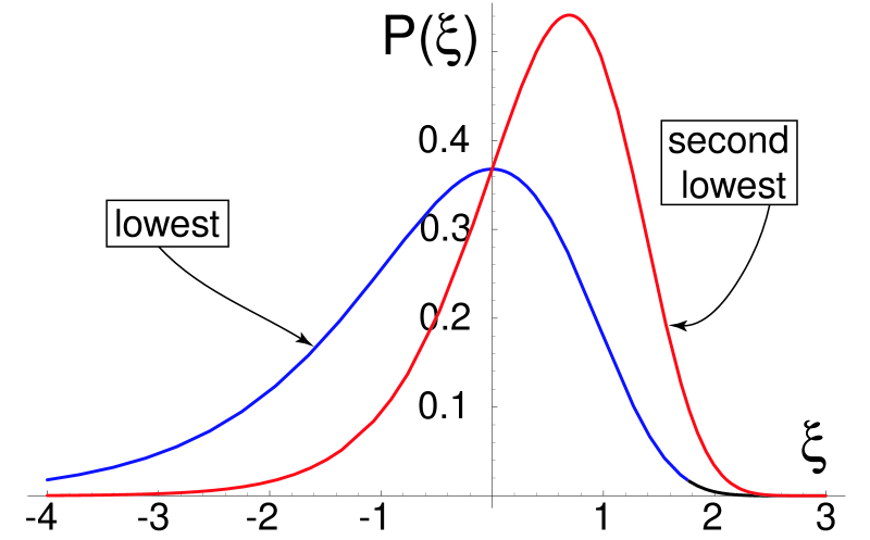
Figure 4: Probability distributions for the lowest and second lowest energy states in REM. Horizontal axes is $\xi=\epsilon/T_{\rm fr}$, and vertical axes is the probability density for this quantity $\xi$ (so the area under each curve in the figure is unity).

A.3.2 Conditional probability of $E_{2}$ at given $E_{1}$

Suppose ground state energy is fixed at $E_{1}$, what is the probability distribution of $E_{2}$ at the given $E_{1}$? According to the general rules of probabilities, this quantity is equal to

$${\cal W}(\left.E_{2}\right|E_{1}) = \frac{{\cal W}(E_{1},E_{2})}{{\cal W}(E_{1})}$$ (75)

$$= \frac{1}{T_{\rm fr}}e^{(\epsilon_{2}/T_{\rm fr})-\exp(\epsilon_{2}/T_{\rm fr})+\exp(\epsilon_{1}/T_{\rm fr})}\ .$$

For understanding, it is useful to mention that this quantity is normalized by the condition $\int_{E_{1}}^{\infty}{\cal W}(\left.E_{2}\right|E_{1})dE_{2}=1$.

A.3.3 Probability distribution for the gap between lowest and second lowest states

As regards the gap between two lowest energy states, $\Delta E=E_{2}-E_{1}$, its probability distribution is also easily found:

$${\cal W}(\Delta E)$$ (76)

$$= \int_{-\infty}^{\infty}dE_{1}\int_{E_{1}}^{\infty}dE_{2}{\cal W}(E_{1},E_{2})\delta\left(E_{2}-E_{1}-\Delta E\right)$$

$$= \int_{-\infty}^{\infty}{\cal W}(E_{2}-\Delta E,E_{2})dE_{2}$$

$$\simeq \frac{1}{T_{\rm fr}^{2}}\int_{-\infty}^{\infty}\exp\left[\frac{\epsilon_{2}-\Delta E}{T_{\rm fr}}+\frac{\epsilon_{2}}{T_{\rm fr}}-e^{\epsilon_{2}/T_{\rm fr}}\right]d\epsilon_{2}$$

$$= \frac{1}{T_{\rm fr}}e^{-\Delta E/T_{\rm fr}}\int_{0}^{\infty}\xi e^{-\xi}d\xi=\frac{1}{T_{\rm fr}}e^{-\Delta E/T_{\rm fr}}\ .$$

Of course, this is the result for $\Delta E>0$, so in general probability distribution for the gap reads

$${\cal W}(\Delta E)=\left\{\begin{array}[]{lcr}0&{\rm for}&\Delta E<0\\ (1/T_{\rm fr})e^{-\Delta E/T_{\rm fr}}&{\rm for}&\Delta E>0\end{array}\right.$$ (77)

It might seem surprising at the first glance that this probability decays only as exponential, not the sharper $e^{-\exp\xi}$ function. Indeed, if we imagine gap forming as fixing lowest energy at the typical place and then looking at the second lowest level, then the probability of the gap decays in a very sharp, double exponential way. However, if we think differently, that $E_{2}$ is fixed in a typical place, and then gap is determined by where is the $E_{1}$, then the probability of $E_{1}$ going down is just exponential. Thus, from this argument we gain the following insight. The probability of the gap is exponential because the dominant possibility for the gap to be large is having unusually low $E_{1}$ rather than high $E_{2}$. Thus, large gap is typically the result of the low ground state.

A.4 Averages

Using formula (68), it is easy to compute the expectation value of the ground state energy:

$$\left<E_{g}\right> = \int_{-\infty}^{\infty}E{\cal W}(E)dE$$ (78)

$$= E_{m}+T_{\rm fr}\int_{-\infty}^{\infty}\xi e^{\xi-\exp\xi}d\xi$$

$$= E_{m}+\frac{\delta\!B}{\sqrt{2s}}\underbrace{\int_{0}^{\infty}\ln\eta e^{-\eta}d\eta}_{\Gamma^{\prime}(1)\approx-0.6}\ ,$$

where $\xi=\epsilon/T_{\rm fr}$ and $\eta=e^{\xi}$. As a fact of mathematical curiosity, there appears $\Gamma^{\prime}$, the derivative of the Euler $\Gamma$-function - rather infrequent guest in physics calculations. However exotic mathematically, this term is smaller than the logarithmic correction term in (65) and so it must be neglected if the first approximation is used for $E_{m}$.

We can also compute the average value of the second lowest energy:

$$\left<E_{2}\right> = \int_{-\infty}^{\infty}E{\cal W}_{2}(E)dE$$ (79)

$$= E_{m}+T_{\rm fr}\int_{-\infty}^{\infty}\xi e^{2\xi-\exp\xi}d\xi$$

$$= E_{m}+\frac{\delta\!B}{\sqrt{2s}}\underbrace{\int_{0}^{\infty}\eta\ln\eta e^{-\eta}d\eta}_{\Gamma^{\prime}(2)=1+\Gamma^{\prime}(1)\approx 0.4}\ .$$

This is greater than the average ground state energy (78) by just the amount $T_{\rm fr}=\delta\!B/\sqrt{2s}$.

The latter result is also consistent with the fact that the average gap, according to eq. (77) is equal to

$$\langle\Delta E\rangle=T_{\rm fr}=\delta\!B/\sqrt{2s}\ .$$ (80)

References

- Bresler and Talmud (1944a) S. Bresler and D. Talmud, Doklady AN SSSR 47, 326 (1944a).
- Bresler and Talmud (1944b) S. Bresler and D. Talmud, Doklady AN SSSR 47, 367 (1944b).
- Finkelstein and Ptitsyn (2002) A. V. Finkelstein and O. B. Ptitsyn, Protein Physics: A Course of Lectures (Academic Press, 2002).
- Bryngelson and Wolynes (1987) J. D. Bryngelson and P. G. Wolynes, Proc. Natl. Acad. Sci. U.S.A 84, 7524 (1987).
- Shakhnovich and Gutin (1989) E. I. Shakhnovich and A. M. Gutin, Biophys. Chem 34, 187 (1989).
- Derrida (1980) B. Derrida, Phys. Rev. Lett 45, 79 (1980).
- Sfatos and Shakhnovich (1997) C. D. Sfatos and E. I. Shakhnovich, Phys. Rep 288, 77 (1997).
- Oliveberg and Shakhnovich (2006) M. Oliveberg and E. I. Shakhnovich, Curr. Opin. Struct. Biol 16, 68 (2006).
- Geissler et al. (2004) P. L. Geissler, E. I. Shakhnovich, and A. Y. Grosberg, Phys. Rev. E 70, 021802 (2004).
- Khokhlov and Khalatur (1999) A. R. Khokhlov and P. G. Khalatur, Phys. Rev. Lett 82, 3456 (1999).
- Khokhlov and Khalatur (2004) A. R. Khokhlov and P. G. Khalatur, Curr. Opin. Solid. State. Mater. Sci 8, 3 (2004).
- Pande et al. (1997) V. S. Pande, A. Y. Grosberg, and T. Tanaka, Biophys. J 73, 3192 (1997).
- Li et al. (1996) H. Li, R. Helling, C. Tang, and N. Wingreen, Science 273, 666 (1996).
- Reagan and Degrado (1989) L. Reagan and W. F. Degrado, Science 241, 976 (1989).
- Amatori et al. (2005) A. Amatori, G. Tiana, J. F-Borg, A. Trovato, and R. A. Broglia, J. Chem. Phys 123, 054904 (2005).
- Amatori et al. (2006) A. Amatori, J. F-Borg, G. Tiana, and R. A. Broglia, Phys. Rev. E 73, 061905 (2006).
- Pande et al. (2000) V. S. Pande, A. Y. Grosberg, and T. Tanaka, Rev. Mod. Phys 72, 259 (2000).
- Bouchaud and Mezard (1997) J. Bouchaud and M. Mezard, J. Phys. A: Math. Gen 30, 7997 (1997).
- Dill and the others (1995) K. A. Dill et al., Protein Sci 4, 561 (1995).
- Wong and Frishman (2006) P. Wong and D. Frishman, PLoS. Comput. Biol 2, 392 (2006).