Aharonov-Casher effect in a two dimensional hole gas with spin-orbit interaction

Abstract

We study the quantum interference effects induced by the Aharonov-Casher phase in a ring structure in a two-dimensional heavy hole (HH) system with spin-orbit interaction realizable in narrow asymmetric quantum wells. The influence of the spin-orbit interaction strength on the transport is analytically investigated. These analytical results allow us to explain the interference effects as a signature of the Aharonov-Casher Berry phases. Unlike the previous studies on the electron two-dimensional Rashba systems, we find that the frequency of conductance modulations as a function of the spin-orbit strength is not constant but increases for larger spin-orbit splittings. In the limit of thin channel rings (width smaller than Fermi wavelength), we find that the spin-orbit splitting can be greatly increased due to the quantization in the radial direction. We also study the influence of magnetic field considering both limits of small and large Zeeman splittings.

Particles propagating through a coherent nanoscale device acquire a quantum geometric phase which can have important physical consequences. This geometric phase, known as Berry phase,Berry (1984) is acquired through the adiabatic motion of a quantum particle in the system’s parameter space and can have strong effects on the transport properties due to self-interference effects of the quasiparticles when moving in cyclic motion. Its generalization to non-adiabatic motion is known as the Aharonov-Anandan phase.Aharonov and Anadan (1987) A classical example of such geometric phases is the Aharonov-Bohm phase acquired by a particle going around a loop in the presence of a magnetic flux. An important corollary to this phase is the Aharonov-Casher (AC) phase arising from the propagation of an electron in the presence of spin-orbit coupling.Aharonov and Casher (1984) This novel effect has attracted strong interest within the spintronic research community which focuses, among other things, on spin-dependent control through electrical means.Wolf et al. (2001); Zutic et al. (2004)

Spintronics has made its way into many niche technological applications, e.g. magnetic memories or MRAM’s,Parkin (2002) using effects that take place in metals. However, the majority of modern electronic devices are based on semiconductors and more applications will be possible when semiconductor devices can employ the spin degree of freedom as another functional variable in computational processing. The effects of the AC phase on transport through semiconducting ring-structures can be tested in two dimensional gas confined to an asymmetric potential well. Such structures enable an all electrical control of the spins via the Rashba spin-orbit interaction by changing the gate voltage.Bychkov and Rashba (1984); Aronov and Lyanda Geller (1993); Choi et al. (1997); Nitta et al. (1999); Mal’shukov et al. (1999) This spin-interference in a semiconductor ring (see Fig. 1) has been proposed as a way to control spin-polarized currentsFrustaglia and Richter (2004); Tserkovnyak et al. (2006) and as a spin-filter.Molnar et al. (2004) Signatures of the Aharonov-Casher effect have already been experimentally detected,Morpurgo et al. (1998); Konig et al. (2006); Bergsten et al. (2006) and more theoreticalSouma and Nikolic (2004) and experimentalHabib et al. (2006) studies have become available recently.

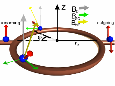
Figure 1: (Color online.) One channel ring of radius $r_{0}$ subject to spin-orbit coupling in the presence of an additional magnetic field $\mathbf{B_{0}}$. Electron (hole) spin travelling around the ring acquires phase due to the applied out-of-plane magnetic field (gray arrow) and the spin-orbit in-plane magnetic field (momentum dependent, green full-line arrows for holes and dashed line arrows for electrons) caused by the spin-orbit interaction. The spin-orbit in-pane magnetic field is different for holes and electrons.

Spin-interference relies on the spin-splitting and, as a result, the devices with stronger spin-splitting can provide more control over the spin. Quantum wells with the spin-orbit interaction proportional to the cube of the momentum (e.g. with a heavy hole (HH) band)Zhang et al. (2001) show, in general, larger spin-orbit splittings. We study here the behavior of the narrow ring in the presence of this cubic spin-orbit interaction. The analysis of recent experiments Konig et al. (2006); Habib et al. (2006) shows that the conductance modulations have larger frequency of oscillations compared to the expected one from a single channel analysis due to Aharonov-Casher effect and it is within a linear-Rashba multi channel conductance analysis that agreement is reached.Konig et al. (2006) In this paper, we analyze whether the larger frequency can be a result of the cubic spin-orbit interaction in a single channel mode. First, we develop a theoretical approach based on the assumption of perfect coupling between leads and the ring. This approach enables us to analytically calculate the Aharonov-Casher modulations of the conductance as a function of the spin-orbit splitting. By introducing an external magnetic field, we also calculate the combined Aharonov-Casher and Aharonov-Bohm conductance modulations. Finally, we study the influence of the Zeeman splitting on the conductance.

The 2D Hamiltonian for a single heavy hole (HH) in the presence of spin-orbit interaction and a magnetic field is given by

$$H_{2D}=\frac{1}{2m^{*}}\bm{\mathbf{\Pi}}^{2}+\frac{1}{2}g\mu_{B}\mathbf{B}\cdot\bm{\mathbf{\sigma}}+\frac{\alpha}{\hbar}(\sigma_{+}\Pi_{-}^{3}-\sigma_{-}\Pi_{+}^{3})+V(\mathbf{r}),$$ (1)

where $g$ is the gyromagnetic ratio, $\mu_{B}$ is the Bohr magneton, $\bm{\mathbf{\sigma}}$ is the vector of the Pauli spin matrices, $\bm{\mathbf{\Pi}}=\mathbf{p}+(e/c)\mathbf{A}$, $\mathbf{\Pi}_{\pm}=\mathbf{\Pi}_{x}\pm i\mathbf{\Pi}_{y}$, $\sigma_{\pm}=\sigma_{x}\pm i\sigma_{y}$ and $\mathbf{B}=\bm{\bigtriangledown}\times\mathbf{A}$. The electrostatic potential $V(\mathbf{r})$ defines, e.g., the lateral confining potential of a 2D ballistic conductor which defines the ring structure. One can obtain the one dimensional (1D) Hamiltonian of a heavy hole in a ring following the procedure described in Appendix, also outlined in Ref. Meijer et al., 2002:

$$\begin{array}[]{l}\hat{H}(\Phi)={\displaystyle\frac{\hbar\omega_{0}}{2}}\left(\widetilde{\partial}_{\varphi}\right)^{2}+{\displaystyle\frac{\hbar\omega_{B}}{2}}\sigma_{z}+\\ {\displaystyle\frac{\hbar\omega_{R}}{4}}\left(2(\cos 3\varphi\sigma_{x}+\sin 3\varphi\sigma_{y})\left(\widetilde{\partial}_{\varphi}\right)^{3}\right.\\ +i3(\cos 3\varphi\sigma_{y}-\sin 3\varphi\sigma_{x})\left[{\displaystyle\frac{3r_{0}^{2}}{w^{2}}}+1+3\left(\widetilde{\partial}_{\varphi}\right)^{2}\right]\\ +\left.(\cos 3\varphi\sigma_{x}+\sin 3\varphi\sigma_{y})\left[{\displaystyle\frac{6r_{0}^{2}}{w^{2}}}-7\right]\widetilde{\partial}_{\varphi}\right)\end{array}$$ (2)

where $\widetilde{\partial}_{\varphi}=\left(i\frac{\partial}{\partial\varphi}+\Phi\right)$, $r_{0}$ is the radius of the ring, $w$ is the half width of the ring channel, $\omega_{0}={\displaystyle\frac{\hbar}{mr_{0}^{2}}}$, $\omega_{B}={\displaystyle\frac{g\mu_{B}B_{z}}{\hbar}}$, $\omega_{R}={\displaystyle\frac{2\alpha}{\hbar r_{0}^{3}}}$, $\Phi={\displaystyle\frac{\pi r_{0}^{2}B}{hc/e}}$. Here we follow the notation of Ref. Frustaglia and Richter, 2004 for easier comparison. Note that the Hamiltonian Eq. (2) is Hermitian since the original Hamiltonian used in Appendix is Hermitian.

The general form of an eigen state of the Hamiltonian Eq. (2) reads:

$$\Psi_{n}(\varphi)=e^{in\varphi}\left(\begin{array}[]{c}\chi_{1}\\ {\displaystyle{\chi_{2}e}^{i3\varphi}}\end{array}\right),$$

where the constants $\chi_{1(2)}$ do not depend on the angle $\varphi$. By diagonalizing the corresponding matrix equation for $\chi_{1(2)}$, we can obtain the eigenenergies and eigenstates.

The complete expressions for the eigenstates and their eigenenergies are too cumbersome to be reproduced here, we thus present analytical results for the two most important limits; (i) thin channel rings with $k_{F}w<1$, and (ii) thick channel rings, $k_{F}w>1$, with small Fermi length compared to the radius, $k_{F}r_{0}\gg 1$ (this limit is usually realized in experiments).Konig et al. (2006); Habib et al. (2006) In case (i) of a ring with a very thin channel, the Hamiltonian simplifies to:

$$\begin{array}[]{l}\hat{H}(\Phi)={\displaystyle\frac{\hbar\omega_{0}}{2}}\left(\widetilde{\partial}_{\varphi}\right)^{2}+{\displaystyle\frac{\hbar\omega_{B}}{2}}\sigma_{z}+{\displaystyle\frac{\hbar\omega_{R}}{2}{\displaystyle\frac{3r_{0}^{2}}{w^{2}}}}\\ \times\left((\cos 3\varphi\sigma_{x}+\sin 3\varphi\sigma_{y})\widetilde{\partial}_{\varphi}+{\displaystyle\frac{3i}{2}}(\cos 3\varphi\sigma_{y}-\sin 3\varphi\sigma_{x})\right)\end{array},$$ (3)

with (non-normalized) eigenstates and eigenenergies:

$$\Psi_{n}(\varphi)=e^{in\varphi}\left(\begin{array}[]{c}{\displaystyle\frac{3+2n-2\Phi+{\displaystyle\frac{2}{3}}h\pm\lambda}{Q_{t}(3+2n-2\Phi)}}\\ {\displaystyle e^{i3\varphi}}\end{array}\right),$$ (4)

$$E_{n}={\displaystyle\frac{\hbar\omega_{0}}{4}}\left((3+2n-2\Phi)^{2}/2+{\displaystyle\frac{9}{2}}\pm 3\lambda\right),$$ (5)

where

$$\lambda=\sqrt{{\displaystyle\frac{4}{9}}h^{2}+{\displaystyle\frac{8}{3}}h(\Phi-n-{\displaystyle\frac{3}{2}})+(1+Q_{t}^{2})(3+2n-2\Phi)^{2}},$$

with $Q_{t}={\displaystyle\frac{r_{0}^{2}}{w^{2}}}{\displaystyle\frac{\omega_{R}}{\omega_{0}}}$ and $h=\omega_{B}/\omega_{0}$. We note however that this limit has not been achieved yet experimentally, e.g. $wk_{F}\sim 30$, although perhaps an effectively narrower channel may be present in some experiments due to irregularities in the ring.

Throughout this paper, we only consider the lowest transverse mode, which should be sufficient for answering the question of whether the larger frequency of conductance oscillations can be a result of the cubic spin-orbit interaction. Thus, in the more experimentally relevant limit (ii), the largest terms in the Hamiltonian Eq. (2) can be captured by fixing the radial coordinate in Eq. (15) to the average value $\left\langle R_{0}(r)\right|r\left|R_{0}(r)\right\rangle=r_{0}$, as it was done in Ref. Aronov and Lyanda Geller, 1993, and consequently symmetrizing it (to make it Hermitian) by the following procedure:

$$\begin{array}[]{ll}\hat{H}_{herm}&=(\hat{H}+\hat{H}^{\dagger})/2=\frac{\hbar\omega_{0}}{2}\left(\widetilde{\partial}_{\varphi}\right)^{2}+{\displaystyle\frac{\hbar\omega_{B}}{2}}\sigma_{z}\\ &+{\displaystyle\frac{\hbar\omega_{R}}{4}}\left\{(\cos 3\varphi\sigma_{x}+\sin 3\varphi\sigma_{y}),\left(\widetilde{\partial}_{\varphi}\right)^{3}\right\}\\ &+i{\displaystyle\frac{3\hbar\omega_{R}}{2}}\left[(\cos 3\varphi\sigma_{y}-\sin 3\varphi\sigma_{x}),\left(\widetilde{\partial}_{\varphi}\right)^{2}\right]\\ &+2\hbar\omega_{R}\left\{(\cos 3\varphi\sigma_{x}+\sin 3\varphi\sigma_{y}),\left(\widetilde{\partial}_{\varphi}\right)\right\}\\ \\ \end{array}$$ (6)

where $\left\{...\right\}$ and $\left[...\right]$ mean commutator and anticommutator respectively. Note that in the case of the Rashba Hamiltonian considered in Ref. Meijer et al., 2002 there is no difference between such symmetrization and the perturbative procedure.

The (non-normalized) eigenstates of the Hamiltonian Eq. (6) are:

$$\Psi_{n}(\varphi)=e^{in\varphi}\left(\begin{array}[]{c}{\displaystyle\frac{\sqrt{12m+13}+{\displaystyle\frac{2}{3}}h\pm\lambda}{mQ\sqrt{12m+13}}}\\ {\displaystyle e^{i3\varphi}}\end{array}\right)$$ (7)

where

$$\lambda=\sqrt{{\displaystyle\frac{4}{9}}h^{2}+{\displaystyle\frac{8}{3}}h(\Phi-n-{\displaystyle\frac{3}{2}})+(12m+13)(1+m^{2}Q^{2})},$$

and $m=n^{2}/3+n-1/3+{\displaystyle\Phi(\Phi-2n-3)/3}$ and $Q=\omega_{R}/\omega_{0}$. The associated eigenenergies read:

$$E_{n}=\hbar\omega_{0}\left(6m+11\pm 3\lambda\right)/4.$$ (8)

Note that in general, the Hamiltonian Eq. (6) gives six eigenstates for a fixed Fermi energy ($E_{F}=E_{n}$). In the limit $\bigtriangleup\ll E_{F}$ (where $\bigtriangleup$ is the energy of spin-orbit splitting and $E_{F}$ is the Fermi energy); however, two of the six states have much larger number $n$, and correspond to the unphysical situation when the cubic spin-orbit coupling term dominates the spectrum creating an unphysical downturn in the spectrum, which is truly not present. Hence, these two states are ignored on the basis of this physical reason, i.e. they do not exists in the physical system. It is convenient to describe the four conducting states by increasing real numbers $n_{1-}\leq n_{2-}\leq n_{2+}\leq n_{1+}$, solutions of the equation $E_{F}=E_{n}$ (see Eqs. (5,8)).

We consider a ring symmetrically coupled to two contact leads in order to study the transport properties of the system subject to a low bias voltage in the linear regime. To this end, we calculate the zero-temperature conductance $G$ based on the Landauer formula:

$$G=\frac{e^{2}}{h}\sum_{\nu^{\prime},\nu=1}^{M}{\displaystyle T_{\nu^{\prime}\nu}},$$ (9)

where labels $\nu$ and $\nu^{\prime}$ number the channel and spin. We assume perfect coupling between leads and ring (i.e., fully transparent contacts), neglecting backscattering effects leading to resonances. In this approximation, the incoming spin $\left|\sigma\right\rangle$ propagates coherently along the four available channels, leaving the ring in a mixed spin state $\left|\sigma_{out}\right\rangle=\sum_{i=1,2;s=\pm}\left\langle\Psi_{n_{is}}(0)\right.\left|\sigma\right\rangle\left|\Psi_{n_{is}}(\pi)\right\rangle$. The spin-resolved transmission probabilities can be obtained by use of a complete basis of incoming $\left|\sigma\right\rangle$ and outgoing $\left|\sigma^{\prime}\right\rangle$ spin states,

$$G=\frac{e^{2}}{h}\sum_{\sigma^{\prime}\sigma}|\left\langle\sigma^{\prime}\right.\left|\sigma\right\rangle|^{2}.$$ (10)

In sufficiently large rings, $k_{F}r_{0}\gg 1$ (e.g. $1/k_{F}\sim 4\mbox{nm}$ in a HgTe QW with a heavy hole band)Zhang et al. (2001), the Zeeman splitting for the magnetic fields considered is small compared to other important energy scales. Summing over all spin-states in Eq. (10) and disregarding the Zeeman term in Eq. (6), we obtain the conductance:

$$G = \frac{e^{2}}{h}\left[1-\cos[\pi(n_{1+}-n_{2+})]\left(\frac{(A-1)}{2}\right.\right.$$ (11)

$$+\left.\left.\frac{(A+1)}{2}\cos[2\pi\Phi]\right)\right]$$

where $A=1$ in the limit (i) and $A={\displaystyle\frac{1+m_{1}m_{2}Q^{2}}{\sqrt{1+m_{1}^{2}Q^{2}}\sqrt{1+m_{2}^{2}Q^{2}}}}$ in the limit (ii), $(n_{1+}-n_{2+})$ is the difference between two roots of Eqs. (5,8), and $m_{1(2)}=n_{1(2)}^{2}/3+n_{1(2)}-1/3+{\displaystyle\Phi(\Phi-2n_{1(2)}-3)/3}$.

In the limit (i) of thin channel rings, we can find the difference between the two roots:

$$n_{1+}-n_{2+}=3\sqrt{1+\left({\displaystyle\frac{r_{0}^{2}}{w^{2}}}Q\right)^{2}},$$

which means that by making the ring channel thinner than the Fermi length we can increase the frequency of conductance oscillations by a factor of $3/(k_{F}w)^{2}$ (see Fig. (2a)). This results from the increase in the spin-orbit splitting due to the quantization in the radial direction. Experimental realization of thin channel rings is very difficult and in the rest of the paper we concentrate on the rings in the limit (ii) when $k_{F}w\gtrsim 1$. Although such rings should have more than one conducting channel, we suppose that only one is important. This can be a result of the resonant transmission of this channel, or incoherent transport through the other channels.

In the experimentally relevant limit (ii), for not too large $Q$, we can approximate $(n_{1+}-n_{2+})$ in Eq. (11) as:

$$n_{1+}-n_{2+}\approx 3+{\displaystyle\frac{2}{3}}\left(N_{F}(8+N_{F})-2\right)Q^{2}$$ (12)

where $N_{F}=E_{F}/(\hbar\omega_{0})=(k_{F}r_{0})^{2}/2$.

Figure 2: Conductance-modulations in a 1D ring as a function of the dimensionless spin-orbit strength $Qk_{F}r_{0}$ (note that state of the art experimental systems are in a regime where $Qk_{F}r_{0}\lesssim 0.1$); a) thin heavy hole ring (solid line) is compared to the Rashba ring (dashed line), $(k_{F}w)^{2}=1/2$; b) and c) thick heavy hole ring (solid line) is compared to the Rashba ring (dashed line).

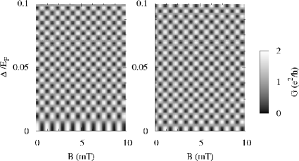
Figure 3: Conductance-modulations in an 1D ring as a function of magnetic field and dimensionless spin-orbit strength (gate voltage). Left plot corresponds to heavy hole spin-orbit interaction, right plot corresponds to Rashba spin-orbit interaction; $r_{0}=1\mu\mbox{m}$, $1/k_{F}\sim 4\mbox{nm}$, $g=20$ and $m^{*}=0.031m$. Parameters of the left plot correspond to the experimental setup in Ref. Konig et al., 2006.

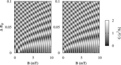
Figure 4: Conductance-modulations in an 1D ring as a function of magnetic field and dimensionless spin-orbit strength (gate voltage) with enhanced Zeeman splitting (multiplied by $10^{3}$). Left plot corresponds to heavy hole spin-orbit interaction, right plot corresponds to Rashba spin-orbit interaction; $r_{0}=1\mu\mbox{m}$, $1/k_{F}\sim 4\mbox{nm}$, $g=20$ and $m^{*}=0.031m$. Parameters of the left plot could correspond to the experimental setup in Ref. Konig et al., 2006 with the magnetic field (range $1-10\>\mbox{T}$) applied under some small angle.

When the parameter $A=1$, Eq. (11) is also valid for an electron ring considered in Ref. Frustaglia and Richter, 2004. This can be obtained by using Eq. (10) and electron Hamiltonian considered in Ref. Frustaglia and Richter, 2004. For the Rashba ring, the difference between roots can be calculated exactly $n_{1+}-n_{2+}=\sqrt{1+Q_{e}^{2}}$ and $Q_{e}={\displaystyle\frac{2m\alpha_{e}r_{0}}{\hbar^{2}}}$ ($\alpha_{e}$ is the Rashba coupling parameter that differs from the one used in Eq. (1)). When the spin-orbit splittings in the hole ($\Delta/E_{F}\sim\sqrt{2N_{F}}Q$) and electron ($\Delta_{e}/E_{F}\sim Q_{e}/\sqrt{2N_{F}}$) systems match, we can write $Q_{e}\sim 2N_{F}Q$. Therefore, the conductance oscillations as a function of spin-orbit splitting for the electron and hole systems have comparable periods (see Figs. 2 and 3)). The period of the hole system has a tendency to become shorter as the spin-orbit splitting becomes larger (see Fig. 2) which is not the case for Rashba rings. Notably, a hole (electron) does not develop sufficient phase difference in the case when the ring radius is small compared to the Fermi length, as it can be seen from Fig. 2. However, as pointed out before, in realistic systems we always have $k_{F}r_{0}\gg 1$ ($1/k_{F}\sim 4\mbox{nm}$ for a HgTe QW with a heavy hole band).Zhang et al. (2001) In Fig. 3, we plot the conductance oscillations in the HH ring (left plot) compared to the Rashba ring (right plot) as a function of the external magnetic field. Here the small g-factor of the electron system is assumed to be the same as for the hole system for easier comparison. Where as in the field direction there is not a large difference in the conductance fluctuations, the changing oscillation frequency of the hole system becomes more obvious as compared to the electron system.

We next take into account the Zeeman splitting as a first order correction. The perturbed eigenenergies become:

$$E_{n} = \frac{\hbar\omega_{0}}{4}\left(6m+11\pm 3\sqrt{(12m+13)(1+m^{2}Q^{2})}\right)$$ (13)

$$\mp{\displaystyle\frac{h\>\mbox{sign}(n)}{2\sqrt{1+m^{2}Q^{2}}}}.$$

where $h=\omega_{B}/\omega_{0}$, sign is the sign function. To the first order in the spin-orbit interaction and Zeeman splitting, Eq. (11) can still describe the conductance after the following substitution:

$$n_{1+}-n_{2+} \rightarrow n_{1+}-n_{2+}+\frac{h}{\sqrt{1+\bar{m}^{2}Q^{2}}}/\left(\frac{\partial E_{n}}{\partial n}\right)$$ (14)

$$\approx n_{1+}-n_{2+}-\frac{h}{\bar{n}\sqrt{1+\bar{m}^{2}Q^{2}}},$$

where $\bar{n}$ is the average of $n_{1+}$ and $n_{2+}$ and $\bar{m}(\bar{n})$ is defined the same way as in Eq. (7). For small Zeeman splittings ($h/n\ll 1$), which holds for realistic rings, the conductance is well described by Eq. (11) and the chessboard pattern in Fig. 2.

We present the results of calculations for larger Zeeman splittings ($h/n\sim 1$) in Fig. 4. The analytical expressions are too cumbersome and we do not reproduce them here. As one can see, the Zeeman term can substantially delay the development of Aharonov-Casher oscillations, especially for larger magnetic fields. In order to experimentally realize this situation, one may apply much larger magnetic fields at some angle to the plane of the ring. Such procedure diminishes the magnetic flux through the structure, allowing to work at higher magnetic fields with much larger Zeeman splittings.

Given the fact that for the experiments in Ref. Konig et al., 2006 and Habib et al., 2006 the experimental systems are in a regime where $Qk_{F}r_{0}\lesssim 0.1$ and $k_{F}w>1$, the frequency of conductance oscillation expected for a single mode (1D) ring are of similar order for both the hole and electron systems. We conclude that the multichannel analysis of the experiments is an important feature for understanding them at present. The increasing frequency of oscillation observed in our calculation, only seen theoretically in the hole gas systems, will require a strength of doping and confining electric field which has not been experimentally achieved at present.

Acknowledgments. The authors are grateful for useful discussions with B. Habib, and M. Shayegan. This work was supported by ONR under Grant No. ONR-N000140610122 and by the NSF under Grant no. DMR-0547875, by the EPSRC through Grant No. GR/S81407/01, by the Grant Agency and Academy of Sciences of the Czech Republic through Grants No. 202/05/0575, and AV0Z10100521, by the Ministry of Education of the Czech Republic Grant No. LC510, by the EU Project NANOSPIN FP6-2002-IST-015728, and from the EU EUROCORES Project SPICO FON/06/E002. M.F.B. is supported by the Department of Education through a GAANN fellowship. Jairo Sinova is a Cottrell Scholar of Research Foundation.

Appendix A Derivation of the 1D Hamiltonian

In this Appendix, we present the derivation of the 1D Hamiltonian for the hole ring. In cylindrical coordinates, with $x=r\cos\phi$ and $y=r\sin\phi$, Eq. (1) reads

$$\begin{array}[]{l}\widehat{H}(r,\phi)=-\frac{\hbar}{2m}\left(\frac{\partial^{2}}{\partial r^{2}}+\frac{\partial}{r\partial r}-\frac{1}{r^{2}}\left(i\frac{\partial}{\partial\phi}+\Phi\right)^{2}\right)+V(r)+\frac{\alpha i}{\hbar r^{3}}\text{cos}[3\phi]\left(3r\left(\sigma_{y}-i\sigma_{x}\Phi+\sigma_{y}\Phi^{2}\right)\frac{\partial}{\partial r}-3r^{2}(\sigma_{y}-i\sigma_{x}\Phi)\frac{\partial^{2}}{\partial r^{2}}\right.\\ +r^{3}\sigma_{y}\frac{\partial^{3}}{\partial r^{3}}-8\sigma_{x}\frac{\partial}{\partial\phi}-6i\sigma_{y}\Phi\frac{\partial}{\partial\phi}+9r\sigma_{x}\frac{\partial^{2}}{\partial\phi\partial r}+6ir\sigma_{y}\Phi\frac{\partial^{2}}{\partial\phi\partial r}-3r^{2}\sigma_{x}\frac{\partial^{3}}{\partial\phi\partial r^{2}}+6\sigma_{y}\frac{\partial^{2}}{\partial\phi^{2}}\left.-3r\sigma_{y}\frac{\partial^{3}}{\partial\phi^{2}\partial r}+i\sigma_{x}\left(i\frac{\partial}{\partial\phi}+\Phi\right)^{3}\right)\\ -\frac{\alpha i}{\hbar r^{3}}\text{sin}[3\phi]\left(3r\left(\sigma_{x}+i\sigma_{y}\Phi+\sigma_{x}\Phi^{2}\right)\frac{\partial}{\partial r}-3r^{2}(\sigma_{x}+i\sigma_{y}\Phi)\frac{\partial^{2}}{\partial r^{2}}\right.+r^{3}\sigma_{x}\frac{\partial^{3}}{\partial r^{3}}+8\sigma_{y}\frac{\partial}{\partial\phi}-6i\sigma_{x}\Phi\frac{\partial}{\partial\phi}-9r\sigma_{y}\frac{\partial^{2}}{\partial\phi\partial r}+6ir\sigma_{x}\Phi\frac{\partial^{2}}{\partial\phi\partial r}\\ +3r^{2}\sigma_{y}\frac{\partial^{3}}{\partial\phi\partial r^{2}}+6\sigma_{x}\frac{\partial^{2}}{\partial\phi^{2}}\left.-3r\sigma_{x}\frac{\partial^{3}}{\partial\phi^{2}\partial r}-i\sigma_{y}\left(i\frac{\partial}{\partial\phi}+\Phi\right)^{3}\right)\end{array}$$ (15)

where $\Phi$ is the magnetic flux through the ring as a function of the radial coordinate, $\Phi={\displaystyle\frac{\pi r^{2}B}{hc/e}}$. We employ the perturbative method used in Ref. Meijer et al., 2002 by separating the Hamiltonian Eq. (15) into the dominant part:

$$\widehat{H}_{0}(r,\phi)=-\frac{\hbar}{2m}\left(\frac{\partial^{2}}{\partial r^{2}}+\frac{\partial}{r\partial r}-\frac{1}{r^{2}}\left(i\frac{\partial}{\partial\phi}+\Phi\right)^{2}\right)+V(r)$$

and the remaining perturbation $\widehat{H}_{1}=\widehat{H}-\widehat{H}_{0}$. In the limit $w\ll r_{0}$ the solution of the Hamiltonian $\widehat{H}_{0}$ can be found as a degenerate set of states $\Psi(r,\phi)=R_{0}(r)\Phi_{n}(\phi)$ where $R_{0}(r)$ is the lowest radial mode and $\Phi_{n}(\phi)$ is a spinor function of the angle $\phi$. It can be shown that the degeneracy in spin space can be lifted by diagonalizing the following Hamiltonian:

$$\widehat{H}_{1D}(\phi)=\left\langle R_{0}(r)\right|\widehat{H}_{1}+\frac{\hbar}{2mr^{2}}\left(i\frac{\partial}{\partial\phi}+\Phi\right)^{2}\left|R_{0}(r)\right\rangle,$$

which allows us to find the desired 1D Hamiltonian.

We use the lowest radial solution found in Ref. Meijer et al., 2002, $R_{0}(r)={\displaystyle\left(\frac{1}{wr_{0}\sqrt{\pi/2}}\right)^{1/2}e^{-(r-r_{0})^{2}/w^{2}}}$, leading to the following expectation values, $\left\langle R_{0}(r)\right|\frac{\partial}{\partial r}\left|R_{0}(r)\right\rangle=-1/(2r_{0})$, $\left\langle R_{0}(r)\right|\frac{\partial}{r^{2}\partial r}\left|R_{0}(r)\right\rangle=1/(2r_{0})$, $\left\langle R_{0}(r)\right|r^{2}\frac{\partial}{\partial r}\left|R_{0}(r)\right\rangle=-3r_{0}/2$, $\left\langle R_{0}(r)\right|\frac{r\partial^{2}}{\partial r^{2}}\left|R_{0}(r)\right\rangle=1/(4r_{0})-r_{0}/w^{2}$, $\left\langle R_{0}(r)\right|\frac{\partial^{2}}{r\partial r^{2}}\left|R_{0}(r)\right\rangle=-1/(r_{0}w^{2})$ and $\left\langle R_{0}(r)\right|\frac{\partial^{3}}{\partial r^{3}}\left|R_{0}(r)\right\rangle=3/(2r_{0}w^{2})$. The Hermitian 1D Hamiltonian for the hole ring takes the form of Eq. (2).

References

Berry (1984)
M. V. Berry,
Proc. R. Soc. Lond. 392,
45 (1984).
Aharonov and Anadan (1987)
Y. Aharonov and
J. Anadan,
Phys. Rev. Lett. 58,
1593 (1987).
Aharonov and Casher (1984)
Y. Aharonov and
A. Casher,
Phys. Rev. Lett. 53,
319 (1984).
Wolf et al. (2001)
S. A. Wolf,
D. D. Awschalom,
R. A. Buhrman,
J. M. Daughton,
S. von Molnar,
M. L. Roukes,
A. Y. Chtchelkanova,
and D. M.
Treger, Science
294, 1488 (2001).
Zutic et al. (2004)
I. Zutic,
J. Fabian, and
S. Das Sarma,
Rev. Mod. Phys. 76,
323 (2004).
Parkin (2002)
S. S. P. Parkin,
Applications of Magnetic Nanostructures
(Taylor and Francis, New York, U.S.A,
2002).
Bychkov and Rashba (1984)
Y. A. Bychkov and
E. I. Rashba,
J. Phys. C: Sol. State Phys.
17, 6039 (1984).
Aronov and Lyanda Geller (1993)
A. G. Aronov and
Y. B. Lyanda Geller,
Phys. Rev. Lett. 70,
343 (1993).
Choi et al. (1997)
T. Choi,
S. Y. Cho,
C. M. Ryu, and
C. K. Kim,
Phys. Rev. B 56,
4825 (1997).
Nitta et al. (1999)
J. Nitta,
F. E. Meijer,
and
H. Takayanagi,
Appl. Phys. Lett. 75,
695 (1999).
Mal’shukov et al. (1999)
A. G. Mal’shukov,
V. V. Shlyapin,
and K. A. Chao,
Phys. Rev. B 60,
R2161 (1999).
Frustaglia and Richter (2004)
D. Frustaglia and
K. Richter,
Phys. Rev. B 69,
235310 (2004).
Molnar et al. (2004)
B. Molnar,
F. M. Peeters,
and
P. Vasilopoulos,
Phys. Rev. B 69,
155335 (2004).
Morpurgo et al. (1998)
A. F. Morpurgo,
J. P. Heida,
T. M. Klapwijk,
B. J. van Wees,
and G. Borghs,
Phys. Rev. Lett. 80,
1050 (1998).
Konig et al. (2006)
M. Konig,
A. Tschetschetkin,
E. M. Hankiewicz,
J. Sinova,
V. Hock,
V. Daumer,
M. Schafer,
C. R. Becker,
H. Buhmann, and
L. W. Molenkamp,
Phys. Rev. Lett. 96,
076804 (2006).
Bergsten et al. (2006)
T. Bergsten,
T. Kobayashi,
Y. Sekine, and
J. Nitta,
Phys. Rev. Lett. 97,
196803 (2006).
Souma and Nikolic (2004)
S. Souma and
B. K. Nikolic,
Phys. Rev. B 70,
195346 (2004).
Habib et al. (2006)
B. Habib,
E. Tutuc, and
M. Shayegan,
cond-mat/0612638 (unpublished) (2006).
Zhang et al. (2001)
X. C. Zhang,
A. Pfeuffer-Jeschke,
K. Ortner,
V. Hock,
H. Buhmann,
C. R. Becker,
and G. Landwehr,
Phys. Rev. B 63,
245305 (2001).
Meijer et al. (2002)
F. E. Meijer,
A. F. Morpurgo,
and T. M.
Klapwijk, Phys. Rev. B
66, 033107
(2002).
Tserkovnyak et al. (2006)
Y. Tserkovnyak,
and
A. Brataas,
cond-mat/0611086 (unpublished) (2006).