Influence of Point-like Disorder on the Guiding of Vortices and the Hall Effect in a Washboard Planar Pinning Potential

Abstract

Explicit current-dependent expressions for anisotropic longitudinal and transverse nonlinear magnetoresistivities are represented and analyzed on the basis of a Fokker-Planck approach for two-dimensional single-vortex dynamics in a washboard pinning potential in the presence of point-like disorder. Graphical analysis of the resistive responses is presented both in the current-angle coordinates and in the rotating current scheme. The model describes nonlinear anisotropy effects caused by the competition of point-like (isotropic) and anisotropic pinning. Nonlinear guiding effects are discussed and the critical current anisotropy is analyzed. Gradually increasing the magnitude of isotropic pinning force this theory predicts a gradual decrease of the anisotropy of the magnetoresistivities. The physics of transition from the new scaling relations for anisotropic Hall resistance in the absence of point-like pins to the well-known scaling relations for the point-like disorder is elucidated. This is discussed in terms of a gradual isotropizaton of the guided vortex motion, which is responsible for the existence in a washboard pinning potential of new (with respect to magnetic field reversal) Hall voltages. It is shown that whereas the Hall conductivity is not changed by pinning, the Hall resistivity can change its sign in some current-angle range due to presence of the competition between i- and a-pins.

I INTRODUCTION

The importance of flux-line pinning in preserving the superconductivity in a magnetic field has been generally recognized since the discovery of type-II superconductivity. But till now the mechanism of flux-line pinning and creep in superconductors (and particularly in the high-$T_{c}$ superconductors (HTSC’s)) is still a matter of controversy and great current interest, especially in the cases of strong competition between different types of pins.

One of the open issues in the field is the influence of isotropic point-like disorder on the vortex dynamics in the anisotropic washboard planar pinning potential (PPP) for the case of arbitrary orientation of the transport current with respect to the PPP ”channels” where the guiding of vortices can be realized. The importance of this issue may be substantiated by ubiquitous presence of point-like pins in those high- and low-$T_{c}$ superconductors which were used so far for resistive measurements of the guided vortex motion^1-9.

The first attempt to discuss the influence of isotropic point-like disorder on the guiding of vortices was made by Niessen and Weijsenfeld¹ still in 1969. They studied guided motion in the flux flow regime by measuring transverse voltages of cold-rolled sheets of a Nb-Ta alloy for different magnetic fields H, transport current densities J, temperatures T, and different angles $\alpha$ between the rolling and current direction. The (H,J,T,$\alpha$)-dependences of the cotangent of the angle $\beta$ between the average vortex velocity $\langle\textbf{v}\rangle$ and the vector J direction were presented. For the discussion, a simple theoretical model was suggested, based on the assumption that vortex pinning and guiding can be described in terms of an isotropic pinning force ${\bf F}_{p}^{i}$ plus a pinning force ${\bf F}_{p}^{a}$ with a fixed direction which was perpendicular to the rolling direction. The experimentally observed dependence of the transverse and longitudinal voltages on the magnetic field in the flux flow regime as a function of the angle $\alpha$ was in agreement with this model.

Unfortunately, in spite of the correct description of a geometry of the motive forces of a problem (see below Fig. 1) it was impossible within the flux flow approach¹ to calculate theoretically the nonlinear (J, T, $\alpha$)-dependences of the average pinning forces $\langle{\bf F}_{p}^{i}\rangle$ and $\langle{\bf F}_{p}^{a}\rangle$ which determine the experimentally observed cot$\beta(J,T,\alpha)$ dependences.

The nonlinear guiding problem was exactly solved at first only for the washboard PPP (i.e. for ${\bf F}_{p}^{i}=0$) within the framework of the two-dimensional single-vortex stochastic model of anisotropic pinning based on the Fokker-Planck equation with a concrete form of the pinning potential^10,11. Two main reasons stimulated these theoretical studies. First, in some HTCS’s twins can easily be formed during the crystal growth^2-5,8. Second, in layered HTCS’s the system of interlayers between parallel ab-planes can be considered as a set of unidirectional planar defects which provoke the intrinsic pinning of vortices¹².

Rather simple formulas were derived¹¹ for the experimentally observable nonlinear even$(+)$ and odd$(-)$ (with respect to the magnetic field reversal) longitudinal and transverse magnetoresistivities $\rho_{\|,\perp}^{\pm}(j,\theta,\alpha,\varepsilon)$ as functions of the dimensionless transport current density $j,$ dimensionless temperature $\theta,$ and relative volume fraction $0<\varepsilon<1$ occupied by the parallel twin planes directed at an angle $\alpha$ with respect to the current direction. The $\rho_{\|,\perp}^{\pm}$-formulas were presented as linear combinations of the even and odd parts of the function $\nu(j,\theta,\alpha,\varepsilon)$ which can be considered as the probability of overcoming the potential barrier of the twins¹¹; this made it possible to give a simple physical treatment of the nonlinear regimes of vortex motion (see below item II.C).

Besides the appearance of a relatively large even transverse $\rho_{\perp}^{+}$ resistivity, generated by the guiding of vortices along the channels of the washboard PPP, explicit expressions for two new nonlinear anisotropic Hall resistivities $\rho_{||}^{-}$ and $\rho_{\perp}^{-}$ were derived and analyzed. The physical origin of these odd contributions caused by the subtle interplay between even effect of vortex guiding and the odd Hall effect. Both new resistivities were going to zero in the linear regimes of the vortex motion (i.e. in the thermoactivated flux flow (TAFF) and the ohmic flux flow (FF) regimes) and had a bump-like current or temperature dependence in the vicinity of highly nonlinear resistive transition from the TAFF to the FF. As the new odd resistivities arose due to the Hall effect, their characteristic scale was proportional to the small Hall constant as for ordinary odd Hall effect investigated earlier¹⁰. It was shown¹¹ that appearance of these new odd $\rho_{||,\bot}^{-}$ contributions leads to the new specific angle-dependent ”scaling” relations for the PPP which demonstrate the so-called anomalous Hall behavior in the type-II superconductors.

Here we should to emphasize that the anomalous behavior of the Hall effect in many high-temperature and in some conventional superconductors in the mixed state remains one of the challenging issues in the vortex dynamics^5,12,16. The problem at issues includes several remarkable experimental facts: a) the Hall effect sign reversal in the vortex state with respect to the normal state at temperatures near $\emph{T}_{c}$ and for moderate magnetic fields; b) the Hall resistivity ”scaling” relation $\rho_{\perp}\sim\rho_{\|}^{\beta}$ exists with $1\leq\beta\leq 2$, where $\rho_{\perp}$ is the Hall resistivity and $\rho_{\parallel}$ is the longitudinal resistivity; c) the influence of pinning on the ”Hall anomaly” and scaling relation. Assuming that the ”bare” Hall coefficient $\alpha_{H}$ is constant, two different scaling laws have been derived earlier theoretically for different pinning potentials^11,17. Vinokur et al. have shown¹⁷ that a scaling law $\rho_{\perp}=\delta\rho_{\parallel}^{2}$ (where $\delta=n\alpha_{H}c^{2}/B\Phi_{0}$ is the Hall conductivity, $n=\pm 1$, $c$ is the speed of light, $B$ is the magnetic field and $\Phi_{0}$ is the magnetic flux quantum) is the general feature of any isotropic vortex dynamics with an average pinning force directed along the average vortex velocity vector. Later it was shown¹¹ that for purely anisotropic a-pins that create a washboard planar pinning potential, the form of corresponding ”scaling” relation is highly anisotropic due to the reason that pinning force for a-pins is directed perpendicular to the pinning planes. If $\alpha$ is the angle between parallel pinning planes and direction of the current density vector $\mathbf{j}$, then for $\alpha=0$ the scaling law has the form $\rho_{\bot}=-n(\alpha_{H}/\eta)\rho_{\|}$ ($\eta$ is the vortex viscosity) which was interpreted previously¹¹ as a scaling law with $\beta=1$, whereas for $\alpha=\pi/2$ the scaling relation is more complex¹¹. The $\rho_{\perp}^{-}$, as it is shown in this paper, can be presented as a sum of the three contributions with the different signs. The graphical analysis in Sec. III of this paper represents a some range of the $(\alpha,j)$-values where the theory predicts a nonlinear change of the $\rho_{\perp}^{-}$ sign.

Let us consider another specific feature of the purely anisotropic guiding model^10,11. From the mathematical viewpoint, the nonlinear anisotropic problem, as solved in Ref. 11, reduces to the Fokker-Planck equation of the one-dimensional vortex dynamics¹³ because the vortex motion is unpinned in the direction which is parallel to the PPP channels. As a consequence, a critical current $j_{c}$ exists only for the direction which is strictly perpendicular to the PPP channels ($\alpha=0$); $j_{c}(\alpha)=0$ for any other direction ($0<\alpha\leq\pi/2$). However, the measurements of the magnetoresistivity show^1-8 that $j_{c}(\alpha)>0$ for all $\alpha$ (although $j_{c}(\alpha)$ may be anisotropic). So, in spite of some merits of a model with a washboard PPP, which was the first exactly solvable stochastic nonlinear model of anisotropic pinning, it cannot describe the $j_{c}$-anisotropy of the experimentally measured samples.

Due to this reason later it was suggested^14,20 another simple model, which demonstrates this $j_{c}$-anisotropy for all $\alpha$ on the basis of the bianisotropic pinning potential formed by the sum of two washboard PPP’s in two mutually perpendicular directions. In contradistinction to the nonlinear model with uniaxial PPP¹¹, this bianisotropic nonlinear model predicts a $j_{c}(\alpha)$-anisotropy and relates it to the guiding anisotropy, describing the appearance of two step-like and two bump-like singularities in the $\rho_{\|,\perp}^{+}$ and $\rho_{\|,\perp}^{-}$ (Hall) resistive responses, respectively. Although several proposals to realize experimentally this bianisotropic model were discussed so far¹⁴, the corresponding experiments, however, are still absent.

At the same time, the experimental study of vortex dynamics in the PPP is always accompanied with a presence of a certain level of point-like disorder. So, as far as the analysis of existing experimental data is concerned, none of the present theoretical studies in the limiting cases of purely anisotropic or isotropic pinning are sufficient. The more general approach is needed.

The objective of this paper is to present results of a theory for the calculation of the nonlinear magnetoresistivity tensor at arbitrary value of competition between point-like and anisotropic planar disorder for the case of in-plane geometry of experiment. This approach will give us the experimentally important theoretical model which demonstrates the $j_{c}$-anisotropy for all $\alpha$ and predicts a nonlinear change of the $\rho_{\perp}^{-}$ sign at some set of parameters (without change of the Hall conductivity) due a competition of the washboard PPP and a point-like disorder.

The organization of the article is as follows. In Sec. II we derive main results of the $i+a$ pinning problem and consider two main limiting cases of purely $a$- or $i$-pinning. In Sec. III we represent the graphical analysis of different types of nonlinear responses, in particular, the $(j,\alpha)$ graphs of the $\rho_{\parallel,\perp}^{\pm}$ magnetoresistivities and the resistive response in a rotating current scheme. In Sec. IV we conclude with a general discussion of our results.

II Main relations

II.1 Formulation of the problem.

The Langevin equation for a vortex moving with velocity $\mathbf{v}$ in a magnetic field $\mathbf{B}=\mathbf{n}B$ ($B\equiv|\mathbf{B}|$, $\mathbf{n}=n\mathbf{z}$, $\mathbf{z}$ is the unit vector in the $z$-direction and $n=\pm 1$) has the form

$$\eta_{0}\mathbf{v}+n\alpha_{H}\mathbf{v}\times\mathbf{z}=\mathbf{F}_{L}+\mathbf{F}_{p}^{a}+\mathbf{F}_{p}^{i}+\mathbf{F}_{th},$$ (1)

where $\mathbf{F}_{L}=n(\Phi_{0}/c)\mathbf{j}\times\mathbf{z}$ is the Lorentz force ($\Phi_{0}$ is the magnetic flux quantum, $c$ is the speed of light), $\mathbf{F}_{p}^{a}=-\nabla U_{p}(x)$ is the anisotropic pinning force ($U_{p}(x)$ is the washboard planar pinning potential), $\mathbf{F}_{p}^{i}$ is the isotropic pinning force, induced by uncorrelated point-like disorder , $\mathbf{F}_{th}$ is the thermal fluctuation force, $\eta_{0}$ is the vortex viscosity, and $\alpha_{H}$ is the Hall constant.

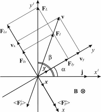
Figure 1: System of coordinates $xy$ (with the unit vectors $\mathbf{x}$ and $\mathbf{y}$) associated with the PPP planes and the system of coordinates $x^{\prime}y^{\prime}$ associated with the direction of the current density vector $\mathbf{j}$; $\alpha$ is the angle between the channels of the PPP and $\mathbf{j}$, $\beta$ is the angle between the average velocity vector of the vortices v and the vector $\mathbf{j}$; $\mathbf{F}_{L}$ is the Lorentz force; $<\mathbf{F}_{p}^{i}>$ and $<\mathbf{F}_{p}^{a}>$ are the average isotropic and anisotropic pinning forces, respectively, $\mathbf{F}_{I}$ is the average effective motive force for a vortex. Here for simplicity we assume $\epsilon=0$.

For purely isotropic pinning (i.e. for $\mathbf{F}_{p}^{a}=0$) Eq. (1) was earlier solved¹⁷ for $\mathbf{F}_{th}=0$, using the fact that

$$\mathbf{F}_{p}^{i}=-\eta_{i}(\upsilon)\mathbf{v},$$ (2)

where $\eta_{i}(\upsilon)$ is velocity-dependent viscosity and $\upsilon\equiv|\mathbf{v}|$.

Below we will show (see Eq. (8) and item D of Sec. II), that the solution, obtained in Ref. 17, can be presented in terms of the probability function of overcoming the effective current- and temperature-dependent potential barrier of isotropic pinning $\nu_{i}(F_{I})$, which is simply related to $\eta_{i}(\upsilon)$.

In the absence of point-like disorder (i.e. for $\mathbf{F}_{p}^{i}=0$) Eq. (1) was reduced to the Fokker-Planck equation, which was solved^10,11, assuming that the fluctuational force $\mathbf{F}_{th}(t)$ is represented by a Gaussian white noise, whose stochastic properties are assigned by the relations

$$\langle F_{th,i}(t)\rangle=0,\,\langle F_{th,i}(t)F_{th,j}(t^{\prime})\rangle=2T\eta_{0}\delta_{ij}\delta(t-t^{\prime}),$$ (3)

where $T$ is the temperature in energy units.

In what follows we derive the solution of Eq. (1), using for $\mathbf{F}_{p}^{i}$ the assumption (2), which reduces Eq. (1) to the equation

$$\eta\mathbf{v}+n\alpha_{H}\mathbf{v}\times\mathbf{z}=\mathbf{F}_{L}+\mathbf{F}_{p}^{a}+\mathbf{F}_{th},$$ (4)

where $\eta=\eta(\upsilon)\equiv\eta_{0}+\eta_{i}(\upsilon)$. Using the result of Ref. 11, the selfconsistent solution of the Eq. (4) can be represented as

$$\begin{array}[]{l}\eta(\upsilon)\langle v_{x}\rangle=F_{a}\nu_{a}(F_{a})/(1+\tilde{\epsilon}^{2}),\\ \\ \eta(\upsilon)\langle v_{y}\rangle=F_{Ly}+n\tilde{\epsilon}F_{a}\nu_{a}(F_{a})/(1+\tilde{\epsilon}^{2}),\end{array}$$ (5)

where $\nu_{a}(F_{a})$ is the probability of overcoming the PPP under the influence the effective moving force $F_{a}\equiv F_{Lx}-n\tilde{\epsilon}F_{Ly}$, $F_{Lx}$ and $F_{Ly}$ are the Lorentz force components acting along the vector $\mathbf{x}$ and $\mathbf{y}$, respectively, $\tilde{\epsilon}\equiv\epsilon Z(\upsilon)$, $\epsilon\equiv\alpha_{H}/\eta_{0}$ and $Z(\upsilon)\equiv\eta_{0}/\eta(\upsilon)$ with an obvious condition $0\leq Z(\upsilon)\leq 1$. Eqs. (5) can be rewritten as

$$\eta(\upsilon)\langle\mathbf{v}\rangle=\mathbf{F}_{I},$$ (6)

where $F_{Ix}$ and $F_{Iy}$ are corresponding right-hand parts of Eqs. (5). From Eq. (6) we have

$$\eta(\upsilon)\upsilon=F_{I},$$ (7)

where $F_{I}\equiv(F_{Ix}^{2}+F_{Iy}^{2})^{1/2}$ and we omitted for simplicity the symbol of averaging for $\mathbf{v}$. Then from Eq. (7) follows that $\upsilon=\upsilon(F_{I})$ and thus it is possible to represent $\eta_{i}(\upsilon)$ and $Z(\upsilon)$ in terms of $F_{I}$: $\eta_{i}(\upsilon)=\eta_{i}[\upsilon=\upsilon(F_{I})]\equiv\tilde{\eta}_{i}(F_{I})$ and

$$Z(\upsilon)=Z[\upsilon=\upsilon(F_{I})]\equiv\nu_{i}(F_{I}).$$ (8)

Here $\nu_{i}(F_{I})$ has a physical meaning of the probability to overcome the effective potential barrier of isotropic pinning under the influence of effective ($\upsilon$-dependent through the $\tilde{\epsilon}$-dependence) force $F_{I}$. Then in terms of the $\nu_{i}(F_{I})$ Eq. (6) takes the selfconsistent form

$$\eta_{0}\mathbf{v}=\nu_{i}(F_{I})\mathbf{F}_{I},$$ (9)

which can be highly simplified for a small dimensionless Hall constant  $(\epsilon\ll 1)$. Really, in this limit  $\tilde{\epsilon}=\epsilon\nu_{i}(F_{i})$, where  $F_{i}\equiv F_{I}(\epsilon=0)$, and the right-hand part of the Eq. (6) becomes $\upsilon$-independent, i.e. is represented only in terms of the known quantities. Just in this limit all subsequent results of the paper will be discussed.

II.2 The nonlinear resistivity and conductivity tensors

The average electric field induced by the moving vortex system is given by

$$\mathbf{E}=(1/c)\mathbf{B}\times\mathbf{v}=n(B/c)(-\upsilon_{y}\mathbf{x}+\upsilon_{x}\mathbf{y}),$$ (10)

where $\mathbf{x}$ and $\mathbf{y}$ are the unit vectors in $x$- and $y$-direction, respectively.

From formulas (9) and (10) we find the dimensionless magnetoresistivity tensor $\hat{\rho}$ (having components measured in units of the flux-flow resistivity $\rho_{f}\equiv\Phi_{0}B/\eta_{0}c^{2}$) for the nonlinear law $\mathbf{E}=\hat{\rho}(j)\mathbf{j}$

$$\begin{array}[]{l}\hat{\rho}=\left(\begin{array}[]{cc}\rho_{xx}&\rho_{xy}\\ \rho_{yx}&\rho_{yy}\end{array}\right)=\\ {}\\ \qquad{}\left(\begin{array}[]{cc}\nu_{i}(F_{I})&-n\epsilon\nu_{i}^{2}(F_{i})\nu_{a}(F_{Lx})\\ n\epsilon\nu_{i}^{2}(F_{i})\nu_{a}(F_{Lx})&\nu_{i}(F_{I})\nu_{a}(F_{a})\end{array}\right).\end{array}$$ (11)

The conductivity tensor $\hat{\sigma}$ (the components of which are measured in units of $1/\rho_{f}$), which is the inverse of the tensor $\hat{\rho}$, has the form

$$\begin{array}[]{l}\hat{\sigma}=\left(\begin{array}[]{cc}\sigma_{xx}&\sigma_{xy}\\ \sigma_{yx}&\sigma_{yy}\end{array}\right)=\\ {}\\ \qquad{}\left(\begin{array}[]{cc}[\nu_{i}(F_{I})]^{-1}&n\epsilon\\ -n\epsilon&[\nu_{i}(F_{I})\nu_{a}(F_{a})]^{-1}\end{array}\right).\end{array}$$ (12)

From Eqs. (11) and (12) we see that the off-diagonal components of the $\hat{\rho}$ and $\hat{\sigma}$ tensors satisfy the Onsager relation ($\rho_{xy}=-\rho_{yx}$ in the general nonlinear case and $\sigma_{xy}=-\sigma_{yx}$). All the components of the $\hat{\rho}$-tensor and the diagonal components of the $\hat{\sigma}$-tensor are functions of the current density $j$ through the external force value $F_{L}$, the temperature $T$, the angle $\alpha$, and the dimensionless Hall parameter $\epsilon$. For the following (see item E.2 of Sec. II) it is important, however, to stress that the off-diagonal components of the $\hat{\sigma}$ (i.e. the dimensional Hall conductivity terms $\delta=n\epsilon/\rho_{f}$) are not influenced by a presence of the $i$- and $a$-pins¹⁶.

The experimentally measurable resistive responses refer to a coordinate system tied to the current (see Fig. 1). The longitudinal and transverse (with respect to the current direction) components of the electric field, $E_{\parallel}$ and $E_{\perp}$, are related to $E_{x}$ and $E_{y}$ by the simple expressions

$$\begin{array}[]{ll}E_{\parallel}=E_{x}\sin\alpha+E_{y}\cos\alpha,\\ \\ E_{\perp}=-E_{x}\cos\alpha+E_{y}\sin\alpha.\\ \end{array}$$ (13)

Then according to Eqs. (13), the expressions for the experimentally observable longitudinal and transverse (with respect to the $\mathbf{j}$-direction ) magnetoresistivities $\rho_{\parallel}\equiv E_{\parallel}/j$ and $\rho_{\perp}\equiv E_{\perp}/j$ have the form:

$$\begin{array}[]{ll}\rho_{\parallel}=\rho_{xx}\sin^{2}\alpha+\rho_{yy}\cos^{2}\alpha,\\ \\ \rho_{\perp}=\rho_{yx}+(\rho_{yy}-\rho_{xx})\sin\alpha\cos\alpha.\\ \end{array}$$ (14)

Note, however, that the magnitudes of the $\rho_{\parallel,\perp}$, given by Eqs. (14), are, in general, depend on the direction of the external magnetic field $\mathbf{B}$ along $z$ axis due to the $n\epsilon$-dependence of the $F_{I}$ and $F_{a}$ forces in arguments of the $\nu_{i}$ and $\nu_{a}$ functions, respectively. In order to consider only $n$-independent magnitudes of the $\rho_{\parallel}$- and $\rho_{\perp}$-resistivities we should introduce the even(+) and the odd($-$) with respect to magnetic field reversal $(\rho^{\pm}\equiv(\rho(n)\pm\rho(-n))/2)$ longitudinal and transverse dimensional magnetoresistivities, which in view of Eqs. (14) have the form:

$$\begin{array}[]{ll}\rho_{\parallel}^{+}=\rho_{f}[\sin^{2}\alpha+\nu_{a}(F_{Lx})\cos^{2}\alpha]\nu_{i}(F_{i}),\\ \\ \rho_{\parallel}^{-}=\rho_{f}[[\sin^{2}\alpha+\nu_{a}(F_{Lx})\cos^{2}\alpha]\nu_{i}^{-}(F_{I})+\\ \\ \qquad{}\nu_{i}(F_{i})\nu_{a}^{-}(F_{a})\cos^{2}\alpha].\\ \end{array}$$ (15)

$$\begin{array}[]{ll}\rho_{\perp}^{+}=-\rho_{f}\nu_{i}(F_{i})[1-\nu_{a}(F_{Lx})]\sin\alpha\cos\alpha,\\ \\ \rho_{\perp}^{-}=\rho_{f}[n\epsilon\nu_{a}(F_{Lx})\nu_{i}^{2}(F_{i})+\\ \\ \qquad\{\nu_{a}^{-}(F_{a})\nu_{i}(F_{i})-\nu_{i}^{-}(F_{I})[1-\nu_{a}(F_{Lx})]\}\times\\ \\ \qquad\qquad\qquad\qquad\qquad\qquad\qquad\qquad\sin\alpha\cos\alpha].\\ \end{array}$$ (16)

Here $\nu^{-}$ are the odd ($\nu^{-}\equiv\nu^{-}(n)=(\nu(n)-\nu(-n))/2$) components of the functions $\nu_{i}(F_{I})$ and $\nu_{a}(F_{a})$, and for $\nu^{-}_{a}(F_{a})$ we have the expansion in terms of $\epsilon<<1$:

$$\nu_{a}^{-}\simeq-n\epsilon\nu_{i}(F_{i})F_{Ly}[d\nu_{a}(F_{Lx})/dF_{Lx}].$$ (17)

Eqs. (15)-(16) are accurate to the first order in $\epsilon<<1$ and contain a lot of new physical information, which will be analyzed below (see item E of Sec. II). However, before this analysis it is instructive to discuss in short the main physically important features of two main limiting cases of purely anisotropic $a$-pinning and isotropic $i$-pinning, which follow from Eqs. (15)-(16), when $\nu_{i}=1$ or $\nu_{a}=1$, respectively.

II.3 Anisotropic a-pinning.

Setting $\nu_{i}=1$ we obtain rather simple formulas, which were derived firstly¹¹ for the experimentally observable nonlinear even and odd longitudinal and transverse anisotropic magnetoresistivities $\rho_{\parallel,\perp}^{\pm}(j,\theta,\alpha,\varepsilon_{a})$ as functions of the transport current density $j$, dimensionless temperature $\theta$ and relative volume fraction $0\leq\varepsilon_{a}\leq 1$, occupied by the parallel twin planes, directed at an angle $\alpha$ with respect to the current direction:

$$\rho_{\parallel a}^{+}=\rho_{f}[\nu_{a}^{+}\cos^{2}\alpha+\sin^{2}\alpha],\quad\rho_{\perp a}^{+}=\rho_{f}(\nu_{a}^{+}-1)\sin\alpha\cos\alpha,$$ (18)

$$\rho_{\parallel a}^{-}=\rho_{f}\nu_{a}^{-}\cos^{2}\alpha,\quad\rho^{-}_{\perp a}=\rho_{f}[n\epsilon\nu_{a}^{+}+\nu_{a}^{-}\sin\alpha\cos\alpha].$$ (19)

Here $\nu_{a}=\nu_{a}(F)$ is considered as the probability of overcoming the potential barrier of the washboard PPP in the $x$-direction under the influence of the effective force $F\equiv F_{Lx}-n\epsilon F_{Ly}$¹¹. This $\nu_{a}$-function describes an essentially nonlinear transition from the linear low-temperature thermoactivated flux flow (TAFF) regime of vortex motion to the ohmic flux flow (FF) regime. It is a step-like function of $j$ or $\theta$ for a small fixed temperature or current density respectively (see Figs. 4, 5 in Ref. 11).

It follows from Eqs. (18)-(19) that for $\alpha\not=0,\pi/2$ the observed resistive response contains not only the ordinary longitudinal $\rho_{||a}^{+}(\alpha)$ and transverse $\rho_{\perp a}^{-}(\alpha)$ magnetoresistivities, but also two new components induced by the pinning anisotropy: an even transverse $\rho_{\perp a}^{+}(\alpha)$ and an odd longitudinal component $\rho_{||a}^{-}(\alpha)$. The physical origin of the $\rho_{\perp a}^{+}(\alpha)$ (which is independent of $\epsilon$) is related in an obvious way with the guided vortex motion along the ”channels” of the washboard pinning potential in the TAFF regime. On the other hand, the component $\rho_{||a}^{-}(\alpha)$ is proportional to the odd component $\nu_{a}^{-}$, which is zero at $\epsilon=0$ and has a maximum in the region of the nonlinear transition from the TAFF to the FF regime at $\epsilon\not=0$ (see Figs. 6, 7 in Ref. 11) The $(j,\theta)$-dependence of the odd transverse (Hall) resistivity $\rho_{\perp a}^{-}(j,\theta)$ has contributions both, from the even $\nu_{a}^{+}\approx\nu_{a}$ and from the odd $\nu_{a}^{-}$ components of the $\nu_{a}(j,\theta)$-function. Their relative magnitudes are determined by the angle $\alpha$ and the effective Hall constant $\epsilon$. Note, that as the odd longitudinal $\rho_{\parallel a}^{-}$ and odd transverse $\rho_{\perp a}^{-}$ magnetoresistivities arise by virtue of the Hall effect, their characteristic scale is proportional to $\epsilon<<1$ (see Eqs. (19)).

The appearance of these new odd Hall contributions follows from emergence of a certain equivalence of $xy$-directions for the case, where a guiding of the vortex along the channels of the washboard anisotropic pinning potential is realized¹⁸ at $\alpha\neq 0,\pi/2$ and leads to the new specific angle-dependent ”scaling” relations for the Hall conductivity¹¹ for the case $\epsilon\tan\alpha<<1$

$$n\epsilon=(\rho_{\perp a}^{-}-\rho_{\parallel a}^{-}\tan\alpha)\cos^{2}\alpha/(\rho_{\parallel a}^{+}-\rho_{f}\sin^{2}\alpha).$$ (20)

Here the dimensionless Hall constant $\epsilon<<1$ is uniquely related to three experimentally observable nonlinear resistivities $\rho_{\parallel a}^{+},\rho_{\parallel a}^{-},\rho_{\perp a}^{-}$, and the ”scaling” relation (20) depends on the angle $\alpha$. This relation differs substantially from the power-law scaling relations, obtained in the isotropic case¹⁷ (see below). In the particular case $\alpha=0$ we regain the results¹⁰, specifically $\epsilon=\rho_{\perp a}^{-}/\rho_{\parallel a}^{+}$ (in Ref. 10 $\epsilon=\rho_{\perp}/\rho_{\parallel}$), i.e. a linear relationship between $\rho_{\perp a}^{-}$ and $\rho_{\parallel a}^{+}$.

Eq. (20) may be represented in another form

$$\rho_{\perp a}^{-}(\alpha)={\delta}\nu_{a}(\alpha){\rho_{f}}^{2}-\rho_{||a}^{-}(\alpha)\tan\alpha$$ (21)

which is more suitable for considering scaling relations in longitudinal ($\alpha=\pi/2$) and transverse ($\alpha=0$) LT-geometries of experiment¹¹. In these geometries second term in the right hand side of Eq. (21) is zero and we obtain that

$$\rho_{\perp a}^{-}=\tilde{\delta}({\rho_{||a}^{+}})^{2},$$ (22)

$$\begin{array}[]{ll}\tilde{\delta}(\alpha=\pi/2)\equiv\tilde{\delta_{L}}={\delta}\nu_{a}(0,\theta);\\ \\ \tilde{\delta}(\alpha=0)\equiv\tilde{\delta_{T}}={\delta}/\nu_{a}(j,\theta).\end{array}$$ (23)

From Eqs. (22)-(23) follows that $\tilde{\delta}$ may be interpreted as an effective Hall conductivity in LT-geometries which is suppressed for $\alpha=\pi/2$ ($\tilde{\delta_{L}}<{\delta}$) and enhanced for $\alpha=0$ ($\tilde{\delta_{T}}>{\delta}$) in comparison with a bare Hall conductivity ${\delta}$. The physical reason for this influence of $\nu_{a}$-function on the $\tilde{\delta}$ behavior in LT-geometries is simple. Namely, it appears as a result of the fact that in the case of anisotropic pinning the driving force $F\equiv F_{Lx}-n\epsilon F_{Ly}$, which determines the probability of overcoming the potential barrier ( and therewith also determines the magnitude of the component of the vortex velocity perpendicular to the channels of the PPP), is the sum of two forces. The first of these is the transverse component of the Lorentz force, $F_{Lx}$= $F_{L}\cos\alpha$, and the other is the transverse component of the Hall force $F_{H}=n\epsilon F_{Ly}$ which is proportional to the longitudinal (relative to the PPP planes) component of the velocity of guided vortex motion. This second force $F_{H}$, which changes its sign (relative to the sign of $F_{L}$ ) upon reversal of the sign of the external magnetic field, is the reason for appearance of new, Hall-like in their origin, $\nu^{-}$-terms in the formulas for the resistive responses in Eqs. (19).

Returning to the physics of suppression and enhancement of the $\tilde{\delta}$ in LT-geometries we should keep in mind that only longitudinal component of the vortex velocity (with respect to the current direction) $v_{l}$ is responsible for the appearance of the transverse Hall voltage. Thus, in L-geometry $v_{l}$ and $\tilde{\delta}$ are suppressed by PPP-barriers, whereas in T-geometry $v_{l}$ is not influenced by them and $\tilde{\delta}$ looks like enhanced quantity. On the contrary, the behavior of the transverse component of the vortex velocity $v_{t}$, which determines the longitudinal voltage, in LT-geometries is opposite.

II.4 Isotropic i-pinning.

For this case we put $\nu_{a}=1$ and from Eqs. (15)-(16) follows that

$$\rho_{\parallel}^{+}=\rho_{\parallel i}=\rho_{f}\nu_{i}(F_{L}),\quad\rho_{\perp}^{-}=\rho_{\perp i}=\rho_{f}n\epsilon\nu_{i}^{2}(F_{L}),$$ (24)

where $F_{L}=F_{i}(\nu_{a}=1)=\mid\mathbf{F}_{L}\mid$. From Eqs. (24) the well-known scaling relation $\rho_{\parallel i}\sim(\rho_{\perp i})^{2}$, derived firstly in Ref. 17, follows. Note that $\rho_{\perp i}^{+}=\rho_{\parallel i}^{-}=0$ in this case, i.e. nonlinear resistive response is isotropic.

II.5 Competition between a- and i-pinning.

Equations (15)-(16) for the magnetoresistivities $\rho_{\parallel,\perp}^{\pm}$ at arbitrary value of competition between point-like and anisotropic planar disorder for the in-plane geometry of experiment can be represented in a more suitable form, if we take into account Eqs. (18)-(19) and (24):

$$\rho_{\parallel}^{+}=\nu_{i}(F_{i})\cdot\rho_{\parallel a}^{+},\quad\rho_{\perp}^{+}=\nu_{i}(F_{i})\cdot\rho_{\perp a}^{+},$$ (25)

$$\rho_{\parallel}^{-}=\nu_{i}^{-}\rho_{\parallel a}^{+}+\nu_{i}(F_{i})\cdot\rho_{\parallel a}^{-},$$ (26)

$$\rho_{\perp}^{-}=\rho_{f}n\epsilon\nu_{a}\nu_{i}^{2}+\rho_{f}\{\nu_{a}^{-}\nu_{i}-\nu^{-}_{i}[1-\nu_{a}]\}\sin 2\alpha/2.$$ (27)

Here $\nu_{i}(F_{i})$ is the probability function $\nu_{i}$ of anisotropic argument $F_{i}=[F^{2}_{Lx}\nu^{2}_{a}(F_{Lx})+F_{Ly}^{2}]^{1/2}$, the magnetoresistivity $\rho_{\parallel,\perp a}^{\pm}$ and the $\nu_{a}\equiv\nu_{a}(F_{Lx})$-functions in Eqs. (25)-(27) are the same as those in item C of Sec. II; $\nu_{i}^{-}=\nu_{i}^{-}[F_{I}(n)]$ and $F_{I}(n)=[F_{Ly}^{2}+F_{Lx}^{2}\nu_{a}^{2}(F_{a})+2n\epsilon\nu_{i}(F_{i})F_{Lx}F_{Ly}\nu_{a}(1-\nu_{a})]^{1/2}$. It is easy to check, that previous results of items C and D of Sec. II follow from Eqs. (25)-(27) in the limits of purely anisotropic (i.e. for $\nu_{i}=1$, $\nu_{i}^{-}=0$) and isotropic (i.e. for $\nu_{a}=1$, $\nu_{a}^{-}=0$) pins.

In this subsection it must be suffice to discuss in short the main physically important features of these equations. First of all, the magnetoresistivities $\rho_{\parallel,\perp}^{\pm}$ can be found, if the $\nu_{a}$- and $\nu_{i}$- functions are known. Moreover, the converse statement is also valid: it is possible to reconstruct these functions from ($j$, $\theta$, $B$)-dependent resistive measurements, using only Eqs. (25), where the Hall terms are ignored. Eqs. (26) and (27), which arise due to the Hall effect, have a rather complicated structure, which reflects a more pronounced competition between isotropic and anisotropic disorder in the Hall-mediated resistive responses. Let us outline the main new physical results, following from Eqs. (25)-(27).

II.5.1 Point-like disorder and vortex guiding.

For the discussion of the influence of point-like pins on the guiding of vortices in the anisotropic pinning potential it is sufficient to analyze Eqs. (25). Whereas for the purely anisotropic pinning ($\nu_{i}=1$) a critical current density $j_{c}$ exists only for direction, which is strictly perpendicular to the PPP ($\alpha=0$) and $j_{c}(\alpha)=0$ for any other direction ($0<\alpha\leq\pi/2$) due to the guiding of vortices along the channels of a washboard potential, in Eqs. (25) the factor $\nu_{i}(F_{i})$ ensures that an anisotropic critical current density $j_{c}(\alpha,\theta)$ exists for arbitrary angles $\alpha$.

It is interesting, however, to note, that the angular dependence of the ratio $\rho_{\perp}/\rho_{\parallel}$, which determines the angle $\beta$ between $\mathbf{j}$ and $\mathbf{v}$ for $a$-pins in Ref. 11, according to the relation

$$\cot\beta=-\frac{\rho_{\perp a}^{+}}{\rho_{\parallel a}}=\frac{1-\nu_{a}}{\tan\alpha+\nu_{a}\cot\alpha}$$ (28)

is not influenced by the isotropic disorder, because factor $\nu_{i}(F_{i})$ in Eqs. (25) vanishes from Eq. (28). Physically it means, that character of anisotropy in the case of competition between $i$- and $a$-pinning is determined only by $<\mathbf{F}_{p}^{a}>=[\nu_{a}(F_{Lx},\theta)-1]\mathbf{F}_{Lx}$, (see Fig. 1), i.e. by the average pinning force of the PPP. Isotropic pins influence only the magnitude of the average $\mathbf{v}$-vector, because $<\mathbf{F}_{p}^{i}>\parallel\mathbf{v}\parallel\mathbf{F}_{I}$. So, the polar resistivity diagram $\rho(\alpha)$, which can be measured experimentally ⁵, is influenced by point-like pins, because from Eqs. (11) follows, that

$$\begin{array}[]{ll}\rho(\alpha)=\rho_{f}[\rho_{xx}^{2}\sin^{2}\alpha+\rho_{yy}^{2}\cos^{2}\alpha]^{1/2}=\\ \\ \qquad{}\rho_{f}\nu_{i}(F_{i})(\sin^{2}\alpha+\nu_{a}^{2}\cos^{2}\alpha)^{1/2}.\\ \end{array}$$ (29)

II.5.2 New Hall voltages and scaling relations.

As it follows from Eqs. (26)-(27), the odd longitudinal $\rho_{\|}^{-}$ and transverse $\rho_{\perp}^{-}$ magnetoresistivities contain terms with the $\nu_{i}^{-}$-function. They possess a highly anisotropic current- and temperature-dependent bump-like behavior. They tend to zero in the linear regime of vortex motion. For $\alpha=0,\pi/2$ these new terms disappear, because $\nu_{i}^{-}=\nu_{a}^{-}=0$ at these limits. As it was in the case of purely a-pinning (see item C of Sec. II), the appearance of these new odd Hall contributions follows from the emergence of a certain equivalence of $xy$-directions due to a guiding of vortices along the channels of the washboard pinning potential for the case with $\alpha\not=0,\pi/2$. Note also, that $\rho_{\|}^{-}$ includes two terms with similar signs, whereas in $\rho_{\perp}^{-}$ there are terms with opposite signs. The latter can give rise to the well-known sign change in the $(j,\theta,H)$-dependence of the Hall resistivity below $\mathrm{T}_{c}$¹².

From Eqs. (25)-(27) new anisotropic ”scaling” relations for the dimensionless Hall constant $\epsilon$ can be derived. For this purpose we exclude $\nu_{i}^{-}$ from Eqs. (25)-(27), for $\nu_{a}^{-}$ use Eq. (17); and after some algebra in the limit $\epsilon\cdot\tan\alpha<<1$ we have:

$$n\epsilon=\frac{2\rho_{\perp}^{-}\cdot\rho_{\parallel}^{+}+\rho_{f}\sin 2\alpha(1-\nu_{a})\nu_{i}\rho_{\parallel}^{-}}{[2\nu_{a}\rho_{\parallel}^{+}-\sin 2\alpha\cdot\rho_{f}\nu_{i}F_{Ly}\nu_{a}^{{}^{\prime}}]\rho_{f}\nu_{i}^{2}}.$$ (30)

It is easy to check that from Eq. (30) follows scaling relations $\delta=n\epsilon/\rho_{f}=\rho_{\perp i}/(\rho_{\parallel i})^{2}$ (for $i$-pins at $\nu_{a}=1$) and Eq. (20) (for $a$-pins at $\nu_{i}=1$)

As it follows from Eqs. (25) and (27), just the same ”scaling” relations as given by Eqs. (22) and (23) for a-pins, exist also for (i+a)-pins (with a replacement of corresponding a-resistivities in Eq. (8) by $\rho_{f}\rho_{\perp}^{-}$ and $\rho_{f}\rho_{\parallel}^{+}$). Physically it follows from the fact that point-like disorder does not change the angular dependence of the ratio $\rho_{\perp a}^{+}/\rho_{\parallel a}^{+}$, which determines the angle $\beta$ between $\mathbf{j}$ and average velocity vector $\langle\mathbf{v}\rangle$ for $a$-pins¹¹, and influences only the magnitude of $\langle\mathbf{v}\rangle$¹⁶.

III Grafical analysis of nonlinear regimes.

III.1 Pinning potential and $\nu$-function behavior.

In order to analyze different types of nonlinear anisotropic $(j,\theta,\alpha)$-dependent magnetoresistivity responses, given by formulas (25)-(27), we should bear in mind that these responses, as is seen from formula (11), are completely determined by the $(j,\theta)$-behavior of the functions $\nu_{a}(F_{a})$ and $\nu_{i}(F_{I})$, having a sense of the probabilities to overcome the effective potential barriers of the $a$- and $i$-pins, respectively. A simple analytical model for the calculation of the $(j,\theta)$-dependent $\nu$-functions was given earlier^11,13,20. We will use for both $\nu_{i}$ and $\nu_{a}$ functions the one-dimensional periodic pinning potential $U_{p}(x)$ (see Fig. 2), which has a simple analytical form^11,20:

$$U_{p}(x)=\left\{\begin{array}[]{crr}\,-F_{p}x,\qquad\qquad 0\leqslant x\leqslant b,\\ \\ F_{p}(x-2b),\qquad b\leqslant x\leqslant 2b,\\ \\ 0,\qquad\qquad\qquad 2b\leqslant x\leqslant h,\\ \end{array}\right.$$ (31)

where $F_{p}$ is the pinning force ($F_{p}=U_{0}/b$, where $U_{0}>0$ is the depth of the potential well and $2b$ is the width of the well). This form of $U_{p}(x)$ allows to define as the properties of a given pinning center (by the parameters $U_{0}$ and $b$), as well as the density of such centers (by the parameter $\varepsilon=2b/h$, where $h$ is the period of the $U_{p}(x)$).

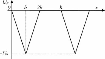
Figure 2: Model pinning potential $U_{p}(x)$: $h$ is the period of the potential, $2b$ is the width of the potential well, $U_{0}$ is the depth of the potential well, $\varepsilon=2b/h$ characterizes the concentration of the pinning planes.

Calculation of the $\nu(j,\theta)$ function on the basis of the pinning potential, given by Eq. (31), was done ¹¹ and can be represented here in the form¹¹

$$\nu(f,\theta,\varepsilon)=\frac{2f(f^{2}-1)^{2}}{2f(f^{2}-1)(f^{2}-1+\varepsilon)-\varepsilon\theta G},$$ (32)

where $G=\{(3f^{2}+1)\cosh(f/\theta\varepsilon)+(f^{2}-1)\cosh[(f(1-\\ \\ \qquad 2\varepsilon))/(\theta\varepsilon)]-2f(f-1)\cosh[f(1-\varepsilon)/\theta\varepsilon-(1/\theta)]-\\ \\ \qquad\quad 2f(f+1)\cosh[(f(1-\varepsilon)/\theta\varepsilon+1/\theta]\}/\sinh(f/\theta\varepsilon).$

Here and below we have for the time being dropped the indices $a$ and $i$ from the physical quantities pertaining to pinning potentials $U_{pa}$ and $U_{pi}$ and formula (32) describes equally the pinning on both potentials. For convenience of qualitative analysis of the formulas following dimensionless parameters were used: $f=Fb/U_{0}$ is the effective motive force, which specifies its ratio to the pinning force $F_{p}=U_{0}/b$, $\theta=T/U_{0}$ is the temperature.

The effect of the external force $F$ acting on the vortices consists in a lowering of the potential barrier for vortices localized at pinning centers and, hence, an increase in their probability of escape from them. Increasing the temperature also leads to an increase in the probability to escape of the vortices from the pinning centers through an increase in the energy of thermal fluctuations of the vortices. Thus the pinning potential of a pinning center, which for $F,T\rightarrow 0$ leads to localization of the vortices, can be suppressed by both an external force and by temperature.

A detailed quantitative and qualitative analysis of the behavior of $\nu(f,\theta,\epsilon)$ as a function of all the parameters and its asymptotic behavior as a function of each are described¹¹. Here we will pay particular attention only to the typical curves of $\nu(f,\theta,\epsilon)$ as a function of the parameters $f$ and $\theta$, which describe the nonlinear dynamics of the vortex system as a function of the external force acting on the vortices in the direction perpendicular to the pinning centers and as a function of temperature (see Figs. $4$ and $5$ in Ref. 11). As we see from those figures, the form of the $\nu(f)$ and $\nu(\theta)$ curves is determined by the values of the fixed parameters $\theta$ and $f$. The monotonically increasing function $\nu(f)$ reflects the nonlinear transition of the vortex motion from the TAFF to the FF regime with the increasing external force at low temperatures ($T\ll U_{0}$), while at high temperatures ($T\gg U_{0})$ the FF regime is realized in the entire range of variation of the external force (even at small forces) because of the effect of thermal fluctuation on the vortices. The monotonically increasing function $\nu(\theta)$ reflects the nonlinear transition from a dynamical state corresponding to the value of the external force at zero temperature to the FF saturation regime. The width of the transition from the TAFF to the FF regime on the $\nu(f)$ and $\nu(\theta)$ curves depends on substantially different on the increasing of the parameters $\theta$ and $f$, respectively. Namely, with increasing $\theta$ the function $\nu(f)$ shifts leftward and becomes less steep (see Fig. 4 in Ref. 11). That is, the higher the temperature, the smoother the transition from the TAFF to the FF regime and the lower the values of the external force, at which it occurs. With increasing $f$ the $\nu(\theta)$ curve also shifts leftward, it becomes steeper (see Fig. 5 in Ref. 11). Consequently, the greater the suppression of the potential barrier of the pinning center by the external force, the sharper the transition from the TAFF to the FF regime and the lower the temperature at which it occurs.

These graphs will be needed later on when we will discuss the physical interpretation of the observed guiding-depended resistive responses. We also note that the dependence of the probability function $\nu(\varepsilon)$ on the concentration of pinning centers decreases monotonically from the value $\nu(0)=1$, which corresponds to the absence of pinning centers, and that it becomes steeper with decreasing fixed parameters $f$ and $\theta$, owing to the growth of the probability density for finding the vortices at the pinning centers with decreasing temperature and external force.

III.2 Dimensionless form of the $\rho_{\parallel,\perp}^{\pm}$-responses.

Let us turn to the dimensionless parameters by which one can in general case take into account the difference of the potentials $U_{a}$ and $U_{i}-$ specifically, the difference of their periods $h_{a}$, $h_{i}$, the potential well depths $U_{0a}$, $U_{0i}$ and the width $b_{a}$, $b_{i}$. We introduce some new parameters: $\varepsilon=(\varepsilon_{a}\varepsilon_{i})^{1/2}$ is the average concentration of pinning centers, $U_{0}=(U_{0a}U_{0i})^{1/2}$ is the average depth of potential well, $\kappa=(\varepsilon_{i}/\varepsilon_{a})^{1/2}=(h_{a}b_{i}/h_{i}b_{a})^{1/2}$, and $p=(U_{0a}/U_{0i})^{1/2}$ , where the parameters $\kappa$ and $p$ are measures of the corresponding anisotropies. The temperature will be characterized by new parameters: $\theta_{a}=pT/U_{0}=T/U_{0a}$ and $\theta_{i}=(1/p)T/U_{0}=T/U_{0i}$, which are the ratio of the energy of thermal fluctuations of the vortices to the average potential well depth $U_{0a}$ and $U_{0i}$, respectively.

The current density will be measured in units of $j_{c}=cU_{0}/\Phi_{0}h$, where $h=(h_{a}h_{i})^{1/2}$. Then the dimensionless parameters $f_{a}$ and $f_{i}$, which specify the ratio of the external forces $F_{a}$ and $F_{i}$ to the pinning forces $F_{pa}=U_{0a}/b_{a}$ and $F_{pi}=U_{0i}/b_{i}$ ($\nu_{a}$ and $\nu_{i}$ are the even functions of their arguments), we denote as $f_{a}=F_{a}/F_{pa}$ and $f_{i}=F_{i}/F_{pi}$. The values of the external force $F$, at which the heights of the potential barriers $U_{0a}$ and $U_{0i}$ vanish at $T=0$ correspond (at $\alpha=0$ and $\alpha=\pi/2$) to the critical current densities $j_{ca}=qj_{c}$ and $j_{ci}=j_{c}/q$ respectively, where $q=p/\kappa$. In general case of nonzero temperature and $0<\alpha<\pi/2$ it is possible to consider the angle-dependent crossover current densities $j_{ca}(\alpha)$ and $j_{ci}(\alpha)$ (see below) which correspond to change in the vortex dynamics from the TAFF regime to a nonlinear regime. The condition, that determines the temperature region, in which the concept of critical current densities is physically meaningful is $0\leqslant T\ll U_{0}$, because for $T\gtrsim U_{0}$ the transition from the TAFF to the nonlinear regime is smeared, and the concept of critical current loses its physical meaning.

It is possible now to rewrite Eqs. (15)-(16) in the dimensionless form in order to represent them as functions of $j$, $\theta$, $\alpha$ at given values of parameters $\varepsilon$, $\epsilon$, $q$, $k$.

$$\rho_{\parallel}^{+}=\nu_{i}(f_{i})[\sin^{2}\alpha+\nu_{a}(f_{a})\cos^{2}\alpha)],$$ (33)

$$\rho_{\perp}^{+}=-\nu_{i}(f_{i})[1-\nu_{a}(f_{a})]\sin 2\alpha/2,$$ (34)

$$\rho_{\parallel}^{-}=\nu_{i}^{-}(\tilde{f_{i}})[\sin^{2}\alpha+\nu_{a}(f_{a})\cos^{2}\alpha)]+\nu_{a}^{-}(\tilde{f_{a}})\nu_{i}(f_{i})\cos^{2}\alpha,$$ (35)

$$\begin{array}[]{l}\rho_{\perp}^{-}=n\epsilon\nu_{a}(f_{a})\nu_{i}^{2}(f_{i})+\\ \\ +\{\nu_{a}^{-}(\tilde{f_{a}})\nu_{i}(f_{i})-\nu^{-}_{i}(\tilde{f_{i}})[1-\nu_{a}(f_{a})]\}\sin 2\alpha/2,\end{array}$$ (36)

$$\textrm{where}\qquad f_{a}=jq^{-1}\cos\alpha,\quad{}\\$$ (37)

$$f_{i}=jq(\sin^{2}\alpha+\nu_{a}^{2}\cos^{2}\alpha)^{1/2},$$ (38)

and   $\tilde{f_{a}}=jq^{-1}[\epsilon\nu_{i}(f_{i})\sin\alpha+n\cos\alpha]$,

$$\begin{array}[]{ll}\tilde{f_{i}}=jq\{\sin^{2}\alpha+\nu_{a}^{2}(\tilde{f_{a}})\cos^{2}\alpha)-n\epsilon\nu_{i}(f_{i})\nu_{a}(f_{a})\times\\ \\ \qquad\qquad\qquad\qquad\qquad\qquad\times[1-\nu_{a}(f_{a})]\sin 2\alpha\}^{1/2}.\end{array}$$

Here

$\nu_{a}(f_{a})=\nu_{a}(f_{a},\theta_{a},\varepsilon_{a}/\kappa)$,  $\nu_{a}(\tilde{f_{a}})=\nu_{a}(\tilde{f_{a}},\theta_{a},\varepsilon_{a}/\kappa)$,
 
    $\nu_{i}(f_{i})=\nu_{i}(f_{i},\theta_{i},\varepsilon_{i}\kappa)$,    $\nu_{i}(\tilde{f_{i}})=\nu_{i}(\tilde{f_{i}},\theta_{i},\varepsilon_{i}\kappa)$,

$$\begin{array}[]{crr}\textrm{and}&\nu^{\pm}_{i}(\widetilde{f}_{i})=\{\nu_{i}[\widetilde{f}_{i}(n)]\pm\nu_{i}[\widetilde{f}_{i}(-n)]\}/2,&\\ \\ &\nu^{\pm}_{a}(\widetilde{f}_{a})=\{\nu_{a}[\widetilde{f}_{a}(n)]\pm\nu_{a}[\widetilde{f}_{a}(-n)]\}/2.&\end{array}$$

In Eqs. (33)-(38) we also denoted $\nu_{i}(f_{i})\equiv\nu^{+}_{i}(\widetilde{f_{i}})$ and $\nu_{a}(f_{a})\equiv\nu^{+}_{a}(\widetilde{f_{a}})$ for simplicity.

Before following graphical analysis of the $\rho_{\parallel,\perp}^{\pm}$ dependences given by Eqs. (33)-(36), we should point out the magnitude of some parameters which will be used for presentation of the graphs. It is important to remind here that the parameter $q$ determines the value of anisotropy between $\nu_{i}$ and $\nu_{a}$ critical current densities, whereas the parameter $k$ describes the anisotropy magnitude of the width of nonlinear transition from the TAFF to the FF regime for $\nu_{i}$ and $\nu_{a}$ function. More definitely, if $q>1$, then $j_{ca}=qj_{c}>j_{ci}=j_{c}/q$ and influence of the $i$-pins on the vortex dynamics decreases with $q$-increasing. For $q<1$ the situation is opposite and anisotropy effects may be fully suppressed with $q$-decreasing. So, for the observation of pronounced competition between $i$- and $a$-pins $q\approx 1$ should be taken.

The temperature dependences of the $\rho_{\parallel}^{+}(\alpha)$ at small current densities under conditions of the presence both isotropic and anisotropic pinning potential were studied experimentally⁸. Arrhenius analysis of these dependences within the frames of suggested here theoretical approach have shown that for the samples⁸ the $U_{0a}=4031$K, $U_{0i}=1568$K, $b_{a}=400$ nm, $b_{i}=2000$ nm at $T\approx 8$K. Then for these samples $q\approx 1.6$, $\kappa\approx 0.5$, $\theta\approx 0.003$. It was also pointed out⁸ that the best fitting of the experimental and theoretical curves was established for $b_{i}/b_{a}=15$, from which follows $\kappa\approx 0.25$. So for all graphs below we used $q=1.6$, $\kappa=0.25$, $\theta=0.003$, $\epsilon=0.01$ and if it is not pointed out specially, $\varepsilon_{a}=1$ and $\varepsilon_{i}=0.1$.

Note also that for the even longitudinal resistivity $\rho^{+}_{\parallel}$ and the even transverse resistivity $\rho^{+}_{\perp}$ for a small Hall effect, terms proportional to $\epsilon\ll 1$ are absent (see Eqs. (33)-(34)) and only contributions describing the competition between isotropic pinning and nonlinear guiding effect on the PPP in terms of the even $\nu_{i}$ and $\nu_{a}$ functions are presented.

III.3 Graphical analysis of current-angular dependences.

III.3.1 $(j,\alpha)$-presentation of $\nu_{a}$ and $\nu_{i}$.

In order to discuss graphical $(j,\alpha)$-behavior of the resistive responses we will use $\nu_{a}$ and $\nu_{i}$ functions of their arguments $f_{a}$ and $f_{i}$, respectively, in the form given by Eq. (32). Then these functions are, as a corresponding $\nu$-function¹¹, the step-functions in $j$ (at fixed $\theta$) or in $\theta$ (at fixed $j$). For every of the $\nu$-functions it is useful to determine the ”crossover current densities” $j_{ci}(\alpha)$ and $j_{ca}(\alpha)$, as those which correspond to the middle point of a sharp step-like nonlinear transition from the TAFF to the FF regime. As it follows from Eqs. (37)-(38), we can present $f_{a}$ and $f_{i}$ as $f_{a}=j/j_{ca}(\alpha)$ with $j_{ca}(\alpha)=q/\cos\alpha$, and $f_{i}=j/j_{ci}(\alpha)$ with $j_{ci}(\alpha)\approx 1/q\cos\alpha$ for $\alpha\ll\pi/4$ and $j_{ci}(\alpha)\approx 1/\nu_{a}q\cos\alpha$ for $\tan^{2}\alpha\ll\nu_{a}^{2}(j,\alpha)$; $j_{ci}(\alpha)\approx 1/q\sin\alpha$ for $\alpha>\pi/4$ because Eq. (38) can be presented in two equivalent forms, namely $f_{i}=jq\cos\alpha\sqrt{\tan\alpha^{2}+\nu_{a}^{2}}=jq\sin\alpha\sqrt{1+(\nu_{a}/\tan\alpha)^{2}}$.

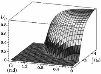
Figure 3: The current-angle dependence of the anisotropic probability function $\nu_{a}(j,\alpha)$. In all following graphs the parameters $q=1.6$, $\kappa=0.25$, $\theta=0.003$, $\epsilon=0.01$, $\varepsilon_{a}=1$, and $\varepsilon_{i}=0.1$ (unless otherwise stated).

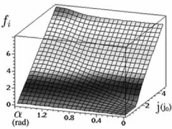
Figure 4: The current-angle dependence of the average effective motive force for a vortex $f_{i}(j,\alpha)$.

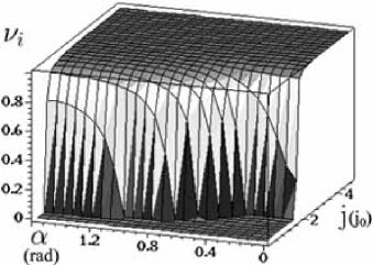
Figure 5: The current-angle dependence of the isotropic probability function $\nu_{i}(j,\alpha)$.

The behavior of $\nu_{a}(j,\alpha)$ function (see Fig. 3) is rather evident from the $f_{a}(j,\alpha)$ behavior. Namely, for all $\alpha\neq\pi/2$ (i.e. for $f_{a}\neq 0$)) the $\nu_{a}$ with a current increasing consistently follows next stages: a) slow increasing at $0<j\lesssim j_{ca}$ in the TAFF regime, where $\nu_{a}\ll 1$, b) sharp step-like increasing with a width of the order of $j_{ca}$ which corresponds to nonlinear transition from the TAFF to the FF regime, c) second stage of slow increasing for $j\gtrsim 2j_{ca}$ which corresponds to the FF regime (see also item C of Sec. II). It follows from the expression for $j_{ca}(\alpha,q)$ that an increasing of $\alpha$ and (or) $q$ leads to a broadening of the step of the order of $j_{ca}$ and its shift to the larger current densities $j\approx j_{ca}$.

The anisotropy of $f_{i}(\alpha)$ (see Eq. (38) and Fig. 4) can be divided into two types: simple (”external”) which depends on $\cos^{2}\alpha$, and more complex (”internal”), given by $\nu_{a}(\alpha)$. The first (external) anisotropy stems from the ”tensorial” $\alpha$-dependence which exists also in the linear (TAFF and FF) regimes of the flux motion. The second (internal) is through the $\alpha$-dependence of $\nu_{a}$, which in the region of transition from the TAFF to the FF regime is substantially nonlinear (Eq. (32) and Fig. 3). The appearance of nonzero $\sin^{2}\alpha$ term in $f_{i}$ for $\alpha\neq 0$ physically describes the guiding of vortices along the channels of the PPP in the presence of $i$-pins for the current densities $j\lesssim~{}j_{ci}(\alpha)$. The influence of $\nu_{a}$-anisotropy on $\nu_{i}$ is different for different values of the angle $\alpha$ (see Fig. 5). For $\alpha>\pi/4$ the anisotropy of $\nu_{a}(\alpha)$ does not influence the value of $f_{i}(\alpha)$ because $(\nu_{a}/\tan\alpha)^{2}\ll 1$ in the expression for $j_{ci}(\alpha)$. On the contrary, for $\alpha\ll\pi/4$ the influence of $a$-pins on $\nu_{i}(\alpha)$ is most effective for that range of current density, where $\nu_{a}^{2}>\tan^{2}\alpha$, due to the inequality $\tan^{2}\alpha\ll 1$. Thus, the $\nu_{i}$ and $\nu_{a}$ as functions of the angle $\alpha$ at $j=const$ behave themselves oppositely (see Figs. 3, 5): $\nu_{i}$ increases monotonically with $\alpha$-increasing, whereas $\nu_{a}$ - monotonically decreases. For $j\gtrsim~{}j_{ca}(\alpha)$ and at small angles which meet the condition $\tan^{2}\alpha\ll 1$, the behavior of the $\nu_{i}$ and $\nu_{a}$ qualitatively similar in $\alpha$ and opposite in $q$.

In case where $\tan^{2}\alpha>1$, the $\nu_{i}$ and $\nu_{a}$ behavior is qualitatively different and stems from the ($\alpha,q$)-dependences of the corresponding crossover current densities. In contradistinction to $\nu_{a}$, the transition of $\nu_{i}$ from the TAFF to the FF depends weakly from $\alpha$ and $q$; it moves to the lower current densities with $q$-increasing for $\alpha>\pi/4$ and moves to the higher ones for $\alpha\ll\pi/4$. In general, the $\nu_{a}$ behavior is more anisotropic than $\nu_{i}$ behavior. The $\nu_{i}$ anisotropy appears only in the TAFF regime, whereas $\nu_{a}$ anisotropy exists as in the TAFF, as well in the FF regime. And this anisotropy is greater in the current density as the angle $\alpha$ is greater. The $\nu_{i}$ and $\nu_{a}$ transition width at $\alpha=const$ is defined by $\varepsilon_{i}$ and $\varepsilon_{a}$ parameters, respectively, and it increases for $\varepsilon_{i}\rightarrow 1$ and $\varepsilon_{a}\rightarrow 1$.

III.3.2 $(j,\alpha)$-presentation of even magnetoresistivities.

Now we are in a position to discuss the results of the presentation of Eq. (25) in the form of graphs. First we note that according to Eqs. (25), the even resistive responses can be represented as the products of corresponding isotropic and anisotropic $\nu$-functions. For this reason the graphical analysis of the $\rho_{\parallel}^{+}(j,\alpha)$ and $\rho_{\perp}^{+}(j,\alpha)$, after the above-mentioned consideration of the $\nu_{i}(j,\alpha)$ (see Fig. 5), can be reduced to the construction and analysis of the $\rho_{\parallel a}^{+}(j,\alpha)$ and $\rho_{\perp a}^{+}(j,\alpha)$ graphs.

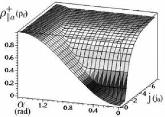
Figure 6: The current-angle dependence of the dimensionless even longitudinal anisotropic magnetoresistivity $\rho_{\parallel a}^{+}(j,\alpha)$ for the value of the parameter $\varepsilon_{a}=1$.

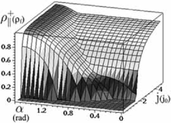
Figure 7: The current-angle dependence of the dimensionless even longitudinal magnetoresistivity $\rho_{\parallel}^{+}(j,\alpha)$ for the value of the parameter $\varepsilon_{a}=1$.

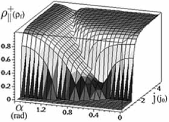
Figure 8: The current-angle dependence of the dimensionless even longitudinal magnetoresistivity $\rho_{\parallel}^{+}(j,\alpha)$ for the value of the parameter $\varepsilon_{a}=0.01$.

Let us begin with a discussion of $\rho_{\parallel a}^{+}$ behavior (see Eq. (18) and Fig. 6). For all $\alpha\neq 0$ due to the term $\sin^{2}\alpha$ in Eq. (18) a critical current density $j_{c}$ exists only for direction, which is strictly perpendicular to the PPP ($\alpha=0$) (as it was shown in item E.1 of Sec. II) and $j_{c}(\alpha)=0$ for any other direction ($0<\alpha\leq\pi/2$) due to the guiding of vortices along the channels of a washboard potential (see also Fig. 8 in Ref. 11). In the FF-regime the isotropization of the $\rho_{\parallel a}^{+}$ arises due to the vortex slipping over the PPP channels. Thus at small angles $\alpha$ the $\nu_{a}$ function strongly influences the $\rho_{\parallel a}^{+}$, whereas for $\alpha\rightarrow\pi/2$ this influence is not so effective due to the external anisotropy, which is proportional to the $\sin^{2}\alpha$ term.

Returning now to the consideration of the $\rho_{\parallel}^{+}(j,\alpha)$ graph we refer to the Eq. (33). It is necessary to pay special attention to the TAFF behavior of these curves at small currents and temperatures, which follows from the full pinning of vortices by point-like pins. This behavior is completely different (for $\alpha\neq 0$) from the non-TAFF behavior of the corresponding graphs for the case of purely anisotropic pinning (see Fig. 8 in Ref. 11), which is provocated by the guiding of vortices along the channels of the PPP. At high current densities and (or) temperatures appears the FF regime, because the vortex motion transverse to the $a$-pins becomes substantial and longitudinal resistivity practically becomes isotropic. In these limiting cases the $\rho^{+}_{\parallel}(j)$ magnitudes are equal to unity (Fig. 7).

For the angles $0<\alpha<\pi/2$ the $\rho_{\parallel}^{+}(j)$ behavior follows substantially the properties of one multiplier. The qualitative behavior of these multipliers, depending on the $j$ and $\alpha$ magnitude is very different as determined by different behavior of their crossover current densities $j_{ci}$ and $j_{ca}$. The priority of a sharp rise of the appearance $\nu_{i}$ or $\nu_{a}$ functions depends on the competition between the crossover current densities $j_{ci}$ and $j_{ca}$, respectively. That is why it may appear a ”step” on some of the $\rho_{\parallel}^{+}(j)$ curves (for $q>1$ and $\alpha\neq 0,\pi/2$) when the next sequence of the vortex motion regimes is realized: a) full $i$-pinning in the TAFF regime ($0<j\lesssim~{}j_{ci}$); b) nonlinear transition from the TAFF to the FF regime for $i$-pins ($j\gtrsim 2j_{ci}$), c) practically linear the FF regime as a consequence of the guiding of vortices along the channels of the washboard PPP (on the $\rho_{\parallel}^{+}(j,\alpha)$ surface one can see the horizontal sections at $j\approx j_{ca}$, see Figs. 7, 8); d) nonlinear transition to the FF regime of vortex motion transverse to the $a$-pins for $j\gtrsim j_{ca}$ and, at last, e) a free FF motion for $j\gg j_{ca}$.

With decreasing of the $q$ the a)-e) corresponding regions along the current density axis $j$ can overlap each other and a common nonlinear transition appears instead of b)-d) regions. For the limiting cases $\alpha=0,~{}\pi/2$, a guiding of vortices is absent and the $\rho_{\parallel}^{+}(j)$ LT-behavior is simply related to the $\nu_{i}$ and $\nu_{a}$ behavior. If parameter $\varepsilon_{a}$ is decreasing, then the width of the transition of $\nu_{a}$ from the TAFF to the FF is also decreasing. Such enhancement of the $\nu_{a}$ steepness leads to appearance of the minimum in $\alpha$ for the $\rho_{\parallel}^{+}(j,\alpha)$ graph (see Fig. 8).

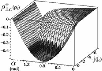
Figure 9: The current-angle dependence of the dimensionless even transverse anisotropic magnetoresistivity $\rho_{\perp a}^{+}(j,\alpha)$

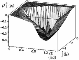
Figure 10: The current-angle dependence of the dimensionless even transverse magnetoresistivity $\rho_{\perp}^{+}(j,\alpha)$. Pay attention to the inverted direction of the axes in comparison with Fig.9.

Now we pass to a discussion of the $\rho_{\perp a}^{+}(j,\alpha)$ and $\rho_{\perp}^{+}(j,\alpha)$ graphs. As it follows from Eq. (18), the $\rho_{\perp a}^{+}<0$ and has a minimum in $\alpha$ for all $j=const$. The $\rho_{\perp a}^{+}$ reaches its maximal magnitude for $\alpha\approx\pi/4$ due to the factor $\sin\alpha\cos\alpha$ and realization of guiding in the TAFF regime for $j\lesssim~{}j_{ca}$ (see. Fig. 9a in Ref. 11 and Fig.9). Therefore, the most favorable angle for its observation is near $\alpha=\pi/4$. In considered case the origin of this minimum has the same reason as a low ($j$, $\alpha$)-behavior of the $\rho^{+}_{\parallel}(j,\alpha)$ curves in Fig. 7, namely it stems from existence of the TAFF regime for the point-like pins at small $j$-values. As is seen in Fig. 9, the position and the magnitude of this $\rho^{+}_{\perp a}$-minimum strongly depends on the $\alpha$-value. It is very much pronounced for $q>1$ and strongly suppressed for $q<1$ by influence of the $i$-pins. With increasing of the current density $j\gtrsim~{}j_{ca}$ a position of the minimum in $\alpha$ is shifting due to the competition of two multipliers in the $\rho_{\perp a}^{+}(j,\alpha)$ expression Eq. (18)): $\sin 2\alpha$ is decreasing for $\alpha\rightarrow\pi/2$, whereas $(1-\nu_{a}(j,\alpha))$ is increasing with $\alpha$-increasing for $j=const$, and decreasing for $j$-increasing for $\alpha=const$ due to the transition to the FF regime. For all $\alpha$ and current densities $j\gtrsim 2j_{ca}$ the $\nu_{a}\approx 1$, and for this reason $\rho_{\perp a}^{+}\rightarrow 0$. The $q$-influence is defined by $j_{ca}(\alpha)$ and determines the region of appearance of a small value of the $\rho_{\perp a}^{+}$ for the current densities $j\approx j_{ca}$.

Since the $\rho_{\perp}^{+}$, according to Eq. (34), is the product of the $\rho_{\perp a}^{+}$ and $\nu_{i}(f_{i})$, so this graph (see Fig. 10) can be reduced to the product of the graphs in Fig. 5 and Fig. 9. The transition from the TAFF to the FF regime is highly anisotropic in $\alpha$; this causes a shift of the maximal $\rho_{\perp}^{+}(j,\alpha)$ magnitude in the direction of a small angle $\alpha\ll\pi/4$ for the $j=const$. That is why in view of $i$-pinning presence the $\rho_{\perp}^{+}(j,\alpha)$, as distinct from $\rho_{\perp a}^{+}(j,\alpha)$, has the minimum both in $\alpha$ and in $j$. This statement follows from the fact that influence of $i$-pinning leads to the $\rho_{\perp}^{+}\rightarrow 0$ for $0<j\lesssim~{}j_{ci}(\alpha)$ due to the $\nu_{i}\ll 1$. For the current densities $j\gtrsim~{}j_{ca}(\alpha)$ the $\rho_{\perp}^{+}(j,\alpha)$ behavior is determined exclusively by the above-mentioned $\rho_{\perp a}^{+}(j,\alpha)$ behavior.

III.3.3 $(j,\alpha)$-presentation of odd magnetoresistivities.

Before following discussion of the odd resistive responses we should remind the reader about the bump-like behavior of the current and temperature dependence of the $\nu^{-}$ functions (see Figs. 6 and 7 in Ref. 11 ), because $\nu^{-}_{i}$ and $\nu^{-}_{a}$ functions, as it follows from Eqs. (35)-(36), give an important contribution to the odd responses. The $\nu^{-}(j)$ and $\nu^{-}(\theta)$ curves for the case of $\epsilon\ll 1$ in fact are proportional to the derivatives of the corresponding $\nu^{+}(j)$ and $\nu^{+}(\theta)$ curves, which have a step-like behavior as a function of their arguments (see Ref. 11 for the detailed discussion of this point and Eq. (17) in this paper). As the $\rho^{-}_{\parallel}$ and $\rho^{-}_{\perp}$ resistivities given by Eqs. (26)-(27) arise by virtue of the Hall effect, their characteristic scale is proportional to $\epsilon\ll 1$, as for Eqs. (19) for purely anisotropic pins.

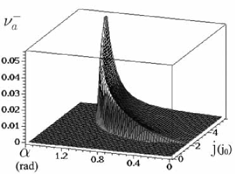
Figure 11: The current-angle dependence of the function $\nu_{a}^{-}(j,\alpha)$.

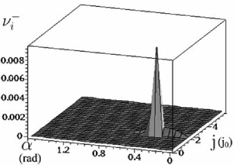
Figure 12: The current-angle dependence of the function $\nu_{i}^{-}(j,\alpha)$.

The position of the characteristic peak in the $\nu^{-}_{i}$ and $\nu^{-}_{a}$ functions is different for $q\neq 1$, because parameter $q$ determines the anisotropy of the critical current densities for $i$- and $a$- pins. So, if $q$ is not very close to the unity, the position of the $i$- and $a$- peaks cannot coincide, and in this case the current and temperature odd resistive dependences $\rho^{-}_{\parallel,\perp}$ can have a bimodal behavior. For the $\rho^{-}_{\parallel}$ curves such dependences will correspond to existence of the resistive ”steps” on the $\rho^{+}_{\parallel}$ curves (see Fig. 7), because for $\epsilon\ll 1$ we can consider the $\rho^{-}_{\parallel}$ dependences as derivatives of the $\rho^{+}_{\parallel}$ curves. From this viewpoint it is easy to understand the previous assertion in item E.2 of Sec. II that $\rho^{-}_{\parallel}$ includes two terms (every proportional to the $\nu^{-}_{i}$ and $\nu^{-}_{a}$, respectively) with similar signs.

Now we will discuss the $\nu_{a}^{-}$ and $\nu_{i}^{-}$ as a function of ($j,\alpha$) and the parameter $q$ in detail. Really, due to the smallness of the Hall constant, the $\nu_{a}^{-}$ and $\nu_{i}^{-}$ tend to zero in the regions of the linear TAFF and FF regimes of the $\nu_{a}$ and $\nu_{i}$ function, respectively. The $\nu_{a}^{-}$ and $\nu_{i}^{-}$ functions have a sharp peak (see Fig. 11, 12) in the region of sharp change of the $\nu_{a}$ and $\nu_{i}$ increasing (for $j\approx j_{ca}$ or $j\approx j_{ci}$, respectively). With $\alpha$- and $q$-increasing the width and the height of the $\nu_{a}^{-}$ maximum also increases with simultaneous shift of the maximum to the higher current densities due to the relation $j_{ca}(\alpha)\approx q/\cos\alpha$. The $\nu_{i}^{-}$ peak is located in the angle range $0<\alpha\lesssim\pi/4$, which corresponds to a change of the angular dependence of the crossover current density $j_{ci}(\alpha)$ from the angles $\alpha\gtrsim\pi/4$ to the angles $\alpha\ll\pi/4$ (see. Fig. 12). The $\nu_{i}^{-}$ maximum shifts to a smaller current densities with $q$-increasing due to the $j_{ci}(\alpha)\approx 1/\nu_{a}q\cos\alpha$,. The magnitudes of the $\nu_{a}^{-}$ and $\nu_{i}^{-}$ are compete by an order of magnitude for $0<\alpha\lesssim\pi/4$ and all $q$-values which satisfy a condition $j_{ca}\approx j_{ci}$.

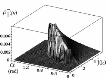
Figure 13: The current-angle dependence of the odd longitudinal magnetoresistivity $\rho_{\parallel}^{-}(j,\alpha)$.

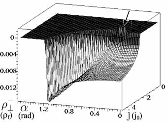
Figure 14: The current-angle dependence of the odd transverse magnetoresistivity $\rho_{\perp}^{-}(j,\alpha)$. The characteristic minimum (which is shown by the arrow) is in the region $0<\alpha<\pi/4$ and $j\approx j_{ci}(\alpha)$. The minimum is shown as two neighboring minimums due to the step-like behavior of the calculation. Pay attention to the inverted direction of the axes in comparison with Fig.13.

Now let us discuss a graphical presentation of the Eq. (35), which can be represented as $\rho_{\parallel}^{-}=B_{1}+B_{2}$, where $B_{1}=\nu_{i}^{-}\rho_{\parallel a}^{+}$, and $B_{2}=\rho_{f}\nu_{a}^{-}\nu_{i}\cos^{2}\alpha$. Taking into account that every factor in the $B_{1}$ and $B_{2}$ is positive (see Figs. 5, 6, 11, 12), we can conclude that $\rho_{\parallel}^{-}\geq 0$ for all values of the $j,\alpha,q$.

Proceeding to the analysis of the $B_{1}$ and $B_{2}$ $(j,\alpha,q)$-behavior in details we consider first those limiting cases in which $a$- or $i$- pinning is dominant i.e. $\nu_{i}\approx 1$ or $\nu_{a}\approx 1$, respectively. If $a$-pinning is dominant (i.e. for $q\gg 1$), then $\nu_{i}^{-}\rightarrow 0$, and Eq.(35) has the form $\rho_{\parallel}^{-}\approx\rho_{\parallel a}^{-}=\nu_{a}^{-}\cos^{2}\alpha$. For the opposite case (i.e. for $q<1$), conversely, $\nu_{a}^{-}\rightarrow 0$, and $\rho_{\parallel}^{-}\approx\nu_{i}^{-}\rho_{\parallel a}^{+}$. The $\rho_{\parallel}^{-}(j,\alpha)$ graph presentation is especially simple because it may be depicted with the aid of Figs. 5, 11, 12.

In the general case, i.e. for $q\approx 1$, we should consider the $B_{1}$ and $B_{2}$ separately because dominant type of pinning is absent. The $B_{1}$ is proportional both $\nu_{i}^{-}$, which is nonzero for $0<\alpha<\pi/4$ and $j(\alpha)\approx j_{ci}(\alpha,q)$ (see Fig. 12), and the factor $\rho_{\parallel a}^{+}$ with a graph, shown in Fig. 6. As a result, the $B_{1}$ has a sharp maximum for the $0<\alpha<\pi/4$ and $j(\alpha)\approx j_{ci}(\alpha,q)$. The second term $B_{2}$ is proportional both the factor $\nu_{a}^{-}$ and the factor $\nu_{i}\cos^{2}\alpha$. The contribution of the first factor is maximal for $\alpha\approx\pi/2$ and current densities $j(\alpha)\approx j_{ca}(\alpha,q)$, whereas the $\nu_{i}\cos^{2}\alpha$ contribution is maximal for $0<\alpha\lesssim\pi/4$ and $j(\alpha)\approx j_{ci}(\alpha,q)$. Therefore these factors compete so that the resulting maximum of $B_{2}$ shifts from $\alpha\approx\pi/2$ to the $\pi/4\lesssim\alpha<\pi/2$. It is relevant to note that the condition $j_{ci}(\alpha)<j_{ca}(\alpha)$ for $q\approx 1$ and $\pi/4\lesssim\alpha<\pi/2$ is always fulfilled. That is why the maximal contribution of the $B_{2}$ is realized for $j(\alpha)\approx j_{ca}(\alpha,q)$ because in this region of the current densities the $\nu_{i}\rightarrow 1$ for $\pi/4\lesssim\alpha<\pi/2$. Therefore the $\rho_{\parallel}^{-}$ behavior is determined mainly by the $B_{2}$ behavior, and the $B_{1}$ contribution is essential for $0<\alpha\lesssim\pi/4$ and $j\approx j_{ci}(\alpha)$.

The $\rho_{\perp}^{-}(j,\alpha)$ dependence is the most complicated. For the sake of simplicity the analysis we represent the $\rho_{\perp}^{-}$ as a sum $\rho_{\perp}^{-}=\rho_{f}[A_{1}+(A_{2}+A_{3})\sin 2\alpha]$, where $A_{1}=n\epsilon\nu_{a}\nu_{i}^{2}$, $A_{2}=\nu_{a}^{-}\nu_{i}/2$, $A_{3}=-\nu^{-}_{i}(1-\nu_{a})/2$. First we consider the limiting cases of purely isotropic or anisotropic pinning ($\nu_{a}\rightarrow 1$ or $\nu_{i}\rightarrow 1$, respectively). For $i$-pinning we have $\rho_{\perp}^{-}=\rho_{f}n\epsilon\nu_{i}^{2}$, from which follows (Vinokur et al.¹⁷) a scaling relation $\rho_{\perp}\sim\rho_{\parallel}^{2}$. For the case of purely anisotropic pinning $\rho_{\perp}^{-}=\rho_{f}\{n\epsilon\nu_{a}+(\nu_{a}^{-}\sin 2\alpha)/2\}$, and the scaling relation is $\rho_{\perp}\sim\rho_{\parallel}$ (see also Ref. 16).

Now we consider every term in the $\rho_{\perp}^{-}(j,\alpha)$ in detail. The $A_{1}$ contribution can be reduced in fact to the multiplication of the graph in Fig. 3 by the graph in Fig. 5 squared; the result is essentially nonzero for $j\gtrsim j_{ca}(\alpha,q)$. The $A_{2}$ contribution was described above (see the $B_{2}$ term in the $\rho_{\parallel}^{-}$ without taking into account the $\cos^{2}\alpha$ anisotropy). Note also that both terms ($A_{1}$ and $A_{2}$) are positive for $n\epsilon>0$. The $A_{3}$ behavior is of great interest because the $A_{3}<0$ for $n\epsilon>0$. Let us consider the cases $q>1$ and $q<1$, which correspond to the $a$-, or $i$-pinning domination, respectively. Then, for $\alpha<\pi/4$:

a) for $q<1$ we have $j_{ci}(\alpha)>j_{ca}(\alpha)$ and the sharp maximum of the $\nu^{-}_{i}$ is suppressed by the factor $(1-\nu_{a})\rightarrow 0$. As a result, the $A_{3}$ contribution can be ignored.

b) for $q\geq 1$ the opposite inequality follows, i.e. $j_{ci}(\alpha)<j_{ca}(\alpha)$. Then for $j\approx j_{ci}(\alpha)$ the $A_{3}$ term is dominant because $\nu_{a}\ll 1$ and $\nu_{i}^{-}\rightarrow n\epsilon$ in this $(j,\alpha)$-region (see Fig. 3 and Fig. 5). As a result, the $\rho_{\perp}^{-}(j,\alpha,q)$ change the sign for $j\approx j_{ci}(\alpha)$ and $0<\alpha\lesssim\pi/4$. Since the scale of the $\nu_{i}^{-}\ll\nu_{i}$, the amplitude of the minimum is small in comparison with the $\rho_{\perp}^{-}$ magnitude.

Thus, a competition of the $a$- and $i$-pinning leads to the qualitatively important conclusion that the $\rho_{\perp}^{-}$ can change its sign at a certain range of $(\alpha,j,q)$-values, namely for $j\approx j_{ci}(\alpha,j,q)$, $0<\alpha\lesssim\pi/4$, and $q>1$.

III.4 Resistive response in a rotating current scheme.

III.4.1 Polar diagram.

An experimental study of the vortex dynamics in $\rm{YBa_{2}Cu_{3}O_{7-\delta}}$ crystals with unidirectional twin planes was recently done using a modified rotating current scheme^4,5. In that scheme it was possible to pass current in an arbitrary direction in the $ab$ plane of the sample by means of four pairs of contacts placed in the plane of the sample. Two pairs of contacts were placed as in the conventional four-contact scheme, and the other two pairs were rotated by $90^{\circ}$ with respect to the first (see the illustration in Fig. $1$ of Ref. 4). By using two current sources connected to outer pair of contacts, one can continuously vary the direction of the current transport in the sample. By simultaneously measuring the voltage in the two directions, one can determine directly the direction and magnitude of the average velocity vector of the vortices in the sample as a function of the direction and magnitude of the transport current density vector. This made it possible to obtain the angular dependence of the resistive response on the direction of the current with respect to the pinning planes on the same sample. The experimental data^4,5 attest to the anisotropy of the vortex dynamics in a certain temperature interval which depends on the value of the magnetic field. A rotating current scheme was used⁴ to measure the polar diagrams of the total magnetoresistivity $\rho(\alpha)$, where $\rho=(\rho^{2}_{x}+\rho^{2}_{y})^{1/2}$ is the absolute value of the magnetoresistivity, $\rho_{x}$ and $\rho_{y}$ are the $x$ and $y$ components of the magnetoresistivity in an $xy$ coordinate system, and $\alpha$ is the angle between the current direction and the $oy$ axis (parallel to the channels of the $a$-pinning centers). In the case of a linear anisotropic response the polar diagram of the resistivity is an ellipse, as can easily be explained. In the case of a nonlinear resistive response the polar diagram of the resistivity is no longer an ellipse and has no simple interpretation.

In this subsection we carry out a theoretical analysis of the polar diagrams of the magnetoresistivity $\rho$ in the general nonlinear case in the framework of a stochastic model of $a+i$ pinning. This type of angular dependence $\rho(\alpha)$ is informative and convenient for theoretical analysis. For a sample with specific internal characteristics of the pinning (such as $q$, $\varepsilon_{a}$, $\varepsilon_{i}$, and $\kappa$) at a given temperature and current density the function $\rho(\alpha)$ is contained by the resistive response of the system in entire region of angles $\alpha$ and makes it possible to compare the resistive response for any direction of the current with respect to the direction of the planar pinning centers. In addition, in view of the symmetric character of the $\rho(\alpha)$ curves, their measurements makes it possible to establish the spatial orientation of the system of the planar pinning centers with respect to the boundaries of the sample if this information is not known beforehand.

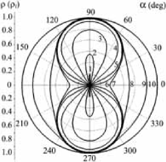
Figure 15: Series of graphs of the function $\rho(\alpha)$ for a sequence of the parameter $j$: 0.63 (1), 0.65 (2), 0.75 (3), 1.00 (4), 1.50 (5), 1.92 (6), 2.00 (7), 2.50 (8), 4.00 (9), 20.0 (10) for $\varepsilon_{a}=1$.

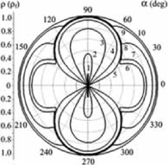
Figure 16: Series of graphs of the function $\rho(\alpha)$ for a sequence of the parameter $j$: 0.63 (1), 0.65 (2), 0.75 (3), 1.00 (4), 1.50 (5), 1.92 (6), 2.00 (7), 2.50 (8), 4.00 (9), 20.0 (10) for $\varepsilon_{a}=0.1$.

Now for analysis of the $\rho(\alpha)$ curves we imagine that vector j is rotated continuously from an angle $\alpha=\pi/2$ to $\alpha=0$. The characteristic form of the $\rho(\alpha)$ curves will obviously be determined by the sequence of dynamical regimes through which the vortex system passes as the current density vector is rotated. By virtue of the symmetry of the problem, the $\rho(\alpha)$ curves can be obtained in all regions of angles $\alpha$ from the parts in the first quadrant.

We recall that in respect to the two systems of pinning centers it is possible to have the linear TAFF and FF regimes of vortex dynamics and regimes of nonlinear transition between them. The regions of nonlinear transitions are determined by the corresponding values of the crossover current densities $j_{ci}(\alpha,q)$ and $j_{ca}(\alpha,q)$.

Now let us consider the typical $\rho(\alpha)$ dependences which are presented in Fig. 15 and 16 for a sequence of a current density magnitude. We remind that the polar diagram graphs represented below are constructed, as the previous graphs in Figs. 3-7, 9-14 for the next values of parameters: $q=1.6$ (i.e. for the case with dominant $a$-pins), $\kappa=0.25$, $\theta=0.003$, $\epsilon=0.01$, $\varepsilon_{i}=0.1$, $\varepsilon_{a}=1$ (Fig. 15), and $\varepsilon_{a}=0.1$ (Fig. 16). Note that $\rho(\alpha)$ is the product of two multipliers: one is the $\nu_{i}(f_{i})$ dependence, which was earlier studied in Fig. 4 of item C.1 of Sec. III, and other is the $\sqrt{\sin^{2}\alpha+\nu_{a}^{2}\cos^{2}\alpha}$ factor, which qualitative behavior is close to the $\rho_{\parallel a}^{+}(j,\alpha)$ dependence (see Fig. 6 in item C.2 of Sec. III).

Let us analyze the $\rho(\alpha)$ behavior for the series of values of the current density $j$. When the angle $\alpha$ changes from $0$ to $\pi/2$ the function $\rho(\alpha)$ grows monotonically from $\rho(0)=\nu_{a}(j/q)\nu_{i}(jq\nu_{a}(j/q))$ to $\rho(\pi/2)=\nu_{i}(jq)$. In Fig. 15 curves 1-6 of the function $\rho(\alpha)$ have the shape of the 8-figure drawn along $ox$-axis (strongly elongated for the curves 1, 2).

This anisotropy can be determined by the relation of the magnitudes of the half-axis at the direction $\alpha=\pi/2$ to the transverse half-axis for any fixed magnitude of the current density. The curves 1-6 of the $\rho=\rho(\alpha)$ graph has the 8-form elongated along $ox$-axis. It is caused by the step-like behavior of the $\nu_{i}$-function, corresponding for the curves 1, 2 to the crossover from the TAFF to the FF regime. That is why the magnitude of the $\rho(\pi/2)$ for the curve 2 is rather greater than for the first one. With $\alpha$-increasing the $\nu_{i}$-function is in the TAFF-region (see Fig.5), which provocates the $\rho(\alpha)\ll 1$ in the case where the condition $j<j_{ci}(\alpha)$ is satisfied. Therefore, with $j$-increasing the magnitude of the angle $\alpha$, which separates the TAFF and the FF regions of the $\nu_{i}$-function at a fixed value of the current density, decreases to the $\alpha\ll 1$.

As the $\nu_{i}(j,\alpha=\pi/2)$ is in the FF region (i.e. $j\gtrsim~{}j_{ci}(\alpha=\pi/2)$), so the anisotropy of the 8-curve decreases for curves 3-6. The $\rho=\rho(\alpha)$ behavior of the curves 5-6 is more isotropic in the region $\alpha\ll\pi/4$ than behavior of the curves 1-4. If the condition $j>j_{ca}(0)$ is satisfied, an appearance of the nonzero resistance in corresponding region follows. Its magnitude is smaller than $\rho(\pi/2)$ for the curves 7, 8, 9 and practically is equal to the $\rho(\pi/2)$ for the curve 10. Note, that for the $\alpha=0,\pi$ and $j_{ca}<j\lesssim 3j_{ca}/2$ one can see the minimum, which decreases with $j$-increasing and disappears in the case where the condition $j\gtrsim 3j_{ca}/2$ is satisfied. So, for large magnitudes of the current densities the $\rho(\alpha)$ behavior becomes more isotropic.

It is necessary to pay attention for the $\rho=\rho(\alpha)$ behavior in the case where $\varepsilon_{a}=0,1$ (see Fig. 16) for the same series of the magnitudes of the current densities. The behavior of the curves 6, 7, 8, 9 differs from the above-mentioned case, but the behavior of the curves 1-5, 10 retains the same. This fact is caused by the influence of the parameter $\varepsilon_{a}$ on the $\nu_{i}$ behavior only in the area of its sharp step-like behavior at the $j\simeq j_{ca}(\alpha)$. Note, that the $\nu_{i}$ contribution is dominant in the region $\alpha\ll 1$ as well as the above-mentioned anisotropy of the $\rho_{\perp a}^{+}(j,\alpha)$ (see Fig. 5 and Fig. 7). As decreasing of the $\varepsilon_{a}$ causes the more narrow crossover from the TAFF- to the FF-regime, the $\nu_{i}(\alpha)$ has a minimum at fixed magnitude of the current density. The magnitude of this minimum decreases with the $j$-increasing and the minimum shifts from the $\alpha\simeq\pi/4$ to the $\alpha\simeq\pi/2$. The influence of the parameter $q$ acts on the crossover current densities $j_{ci}$ and $j_{ca}$ only quantitatively, but does not change an evolution of the curves 1-10 qualitatively.

III.4.2 $\Theta_{E}(\alpha)$-dependence.

Let us examine theoretically in our model a new type of the experimental dependence, recently studied⁴ for $\Theta_{E}(\alpha)$, where $\Theta_{E}$ is the angle between $\mathbf{j}$-vector and the electric field vector $\mathbf{E}$ measured at fixed values of the current density and temperature. Taking into account that in the xy coordinate system the magnetoresistivity components are $\rho_{x}=\rho_{xx}\sin\alpha=\nu_{i}(F_{i})\sin\alpha$, $\rho_{y}=\rho_{yy}\cos\alpha=\nu_{i}(F_{i})\nu_{a}(F_{a})\cos\alpha$, we obtain the following simple relation: $\tan\Theta_{E}(\alpha)=\rho_{x}/\rho_{y}=\tan\alpha/\nu_{a}(F_{a})$, or

$$\Theta_{E}(\alpha)=\arctan(\tan\alpha/\nu_{a}(F_{a})).$$ (39)

Note, that the $\nu_{i}$ term, describing the $i$-pinning, is absent in Eq.(39). Then it follows from the latter that the $\nu_{a}(j,\alpha,\theta)=\tan\alpha/\tan\Theta_{E}(j,\alpha,\theta)$, i.e. the $\nu_{a}(j,\alpha,\theta)$ function can be found from the experimental dependence $\Theta_{E}(\alpha)$. Unfortunately, the dependence $\Theta_{E}(\alpha)$ for the series of the temperature values was experimentally found⁴ so far only for the FF-regime (see. Fig. 2 in Ref. 4). The $\Theta_{E}(j,\alpha)$ dependence is presented in Fig. 17. It shows all changes in the $\Theta_{E}(j,\alpha)$ behavior also for the TAFF-regime.

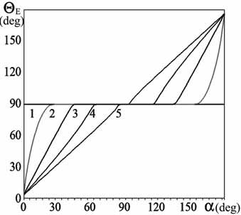
Figure 17: Series of graphs of the function $\Theta_{E}(\alpha)$ for a sequence of the parameter $j$: 1 (1), 1.7 (2), 2.2 (3), 3.5 (4), 20 (5) for $T=8K$.

Let us analyze the Eq. (39) in detail. The $\Theta_{E}(j,\alpha)$ is the odd function of the angle $\alpha$, and its magnitude increases monotonically with the $\alpha$-increasing for all values of the $j$ due to the monotonical decreasing of the $\nu_{a}(j,\alpha)$ function (see. Fig. 17). It follows from Eq. (39) that the period of the function $\Theta_{E}(\alpha)$ is equal to $\pi$. One more important limiting case is realized for $\nu_{a}\approx 1$,which corresponds to the limit of isotropic pinning. Depending on the inequality between the $j$ magnitude and the crossover current density $j_{ca}(\alpha)\approx q/\cos\alpha$, one can separate two regions where the $\Theta_{E}(j,\alpha)$ behavior is qualitatively different. If A is the argument of the arctangent function in Eq. (39), then in that region $j,\alpha,q$, where the inequality $j\gtrsim~{}j_{ca}(\alpha)$ is true (the FF regime for $\nu_{a}(j,\alpha)$, see also Fig. 3), the magnitude of the $\Theta_{E}\approx\emph{A}$ as $\emph{A}\ll 1$. And for the case $j\lesssim~{}j_{ca}$ (the TAFF regime of the $\nu_{a}(j,\alpha)$) the value $\Theta_{E}\approx\pi/2-\emph{A}^{-1}$, as $\emph{A}\gg 1$.

Note, that the parameter $\varepsilon_{a}$ influences the $\Theta_{E}(j,\alpha)$ by changing the character of the step-like crossover of the $\nu_{a}(j,\alpha)$ (the smaller the $\varepsilon_{a}$, the sharper the crossover). The value of the parameter $q$, as well as above-mentioned, determines the magnitude of the $j_{ca}(\alpha)$ (and, therefore the position of the boundaries in $j$ of the regions of quite different $\Theta_{E}(\alpha)$ behavior) at fixed $\alpha$.

III.4.3 Critical current density anisotropy.

Under the critical current density we mean the current density, which corresponds to the electric field strength on the sample $E=1\mu V/cm$. Let us determine the $j_{c}(\alpha)$ behavior graphically by crossing the $E_{\parallel}^{+}=j\rho_{\parallel}^{+}(j)$ graph and the plain $E=E_{c}$ in the polar coordinates. For all angles $\alpha$ the point of crossing for these graphs determines the critical current density magnitude for the defined direction, and the crossing line of the graphs presents the dependence $j_{c}(\alpha)$.

Let us remind the reader that as in above-mentioned sections, in the nonlinear law $E_{\parallel}^{+}=j\rho_{\parallel}^{+}(j)$ we measure $j$ and $\rho$ in the values of the $j_{0}=cU_{0}/\Phi_{0}dh$ and $\rho_{f}=\rho_{n}B/B_{c2}$, respectively. That is why the $E$ magnitude we have to measure in the $E_{0}=j_{0}\rho_{f}$. As well as in item B of Sec. III we use the data from Ref. 8, where for the niobium samples $\rho_{n}\approx 5,5\cdot 10^{-6}$ Ohm$\cdot$cm, $B\approx 150$ Gs, $B_{c2}\approx$ 17 kGs, $\rho_{f}\approx 5\cdot 10^{-8}$Ohm$\cdot$cm, $U_{0}=2500K$, and $d=2.5\cdot 10^{-6}cm$.

Therefore, $E_{0}\approx 6\cdot 10^{-4}V/cm$, and for $E_{c}=1\mu V/cm$ we have to cross the dimensionless $\rho_{\parallel}^{+}(j)\cdot j$ graph by the plain $E\approx 0.002$.

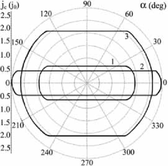
Figure 18: Series of graphs of the function $j_{c}(\alpha)$ for the parameter pairs: $E_{c}=0.002$, $q$=1.6 (1); $E_{c}=0.002$, $q$=3 (2); $E_{c}=2$, $q$=1.6 (3).

Now we will discuss the $j_{c}(\alpha)$ as a function of $\alpha,q,E_{c}$, and $\varepsilon$ in detail. The $j_{c}(\alpha)$-anisotropy can be determined by the relation of the magnitudes of the half-axis at the direction $\alpha=0$ to the transverse half-axis for any fixed magnitude of the parameters $q$, $E_{c}$. The $j_{c}(\alpha)$ decreases monotonically from $j_{c}(0)$ with $\alpha$-increasing and has a minimum for $\alpha=\pi/2$. It is caused by the fact that, as it was shown in item C.1 of Sec. II, the $a$-pinning (with high values of the $j_{ca}$ for $q>1$) does not influence the $i$-pinning for $\alpha=\pi/2$. Therefore, the inequality for the crossover current densities $j_{ci}(\alpha)<j_{ca}(\alpha)$ for $q>1$ leads to the corresponding inequality for the critical current densities $j_{c}(0)<j_{c}(\pi/2)$.

The $q$ influences the $j_{c}(\alpha)$ behavior (as in item D.1 of Sec. II) only quantitatively: with $q$-increasing the ratio $j_{c}(0)/j_{c}(\pi/2)$ grows and visa versa. It is caused by the $j_{c}(0)$-increasing and $j_{c}(\pi/2)$-decreasing due to the $\alpha$-behavior of the corresponding crossover current densities $j_{ci}(\alpha)$ and $j_{ca}(\alpha)$. The smaller the $\varepsilon_{a}$, the sharper the crossover between the $j_{c}(\alpha)$ regions of slowly and quickly decreasing as a function of the $\alpha$. With $E_{c}$-increasing the nonlinear law $E_{\parallel}^{+}=\rho_{\parallel}^{+}(j)j$ is satisfied for the larger values of the current density.

That is why with $\alpha$-increasing from $0$ to $\alpha^{\ast}$ values (for which the condition $\tan^{2}\alpha^{\ast}\ll\nu_{a}^{2}(j,\alpha^{\ast})$ is satisfied) the $\nu_{a}$-function is in the FF regime and $j_{c}(\alpha)$ decreases slowly. When the condition $\alpha>\alpha^{\ast}$ is true the $\nu_{a}$-function has a step-like crossover from the FF to the TAFF regime and $j_{c}(\alpha)$ decreases quickly.

So, the $\alpha^{\ast}$ behavior as a function of the parameters $q$ and $E_{c}$ is qualitatively different: it increases with $E_{c}$-increasing and decreases with $q$-increasing. On the increase of the $E_{c}$ by the several orders of magnitude the $j_{c}(\alpha)$ curve degenerates into a circumference due to the isotropization of the $j_{ci}(\alpha)$ and $j_{ca}(\alpha)$ behavior for the high $j$-values. Otherwise, with $E_{c}$-decreasing the $j_{c}(\alpha)$ curve degenerates into a narrow loop, because the $j_{ci}(\alpha)$ and $j_{ca}(\alpha)$ behavior for a small $j$ is very anisotropic.

IV CONCLUSION.

In the present work we have theoretically examined the strongly nonlinear anisotropic two-dimensional single-vortex dynamics of a superconductor with coexistence of the anisotropic washboard PPP and isotropic pinning potential as function of the transport current density $j$ and the angle $\alpha$ between the direction of the current and PPP planes at a fixed temperature $\theta$.

The experimental realization of the model studied here can be based on both naturally occurring^2-5 and artificially created^6-8 systems with $i+a$ pinning structures. The proposed model has made it possible for the first time (as far as we know) to give a consistent description of the nonlinear anisotropic current- and temperature-induced depinning of vortices for an arbitrary direction relative to the anisotropy of the washboard PPP. In the framework of this model one can successfully analyze theoretically certain observed resistive responses which are used for studying anisotropic pinning in a number of new experimental techniques⁴ (the polar diagram of $\rho(\alpha)$, the $\Theta_{E}(\alpha)$ curve described by formula Eq. (39)) as well as new Hall responses specific for the $i+a$ pinning problem.

A quantitative description of the anisotropic nonlinear resistive properties of the problem under study is done in the framework of the stochastic model on the basis of the Fokker-Planck approach. The main nonlinear components of the problem are the anisotropic $\nu_{a}(F_{a})$ and isotropic $\nu_{i}(F_{i})$ probability functions for the vortices to overcome the potential barriers of $a$- and $i$-pinning centers under the action of anisotropic motive forces $F_{a}$ and $F_{i}$, respectively. The latter include both the ”external” parameters $j,\alpha,\theta$ and the ”internal” parameters $q,\varepsilon_{i},\varepsilon_{a}$ which describe the intensity and anisotropy of the pinning. As can be seen from Eqs. (33)-(36), the magnetoresistivities $\rho_{\parallel,\perp}^{\pm}(j,\alpha,\theta)$ are, in general, nonlinear combinations of the experimentally measured $\nu_{i}$ and $\nu_{a}$ functions ($\nu_{i}$ can be measured independently from the $\rho_{\parallel,\perp}^{+}(\alpha=\pi/2)$, see Eq. (33) and $\nu_{a}$ - from the $\Theta_{E}(\alpha)$, see Eq. (39)).

Therefore, the nonlinear (in $j$) resistive behavior of the vortex system can be caused by factors of both an anisotropic and isotropic pinning origin. It is important to underline that whereas the structure of the $\nu_{a}(F_{a})$ and $F_{a}$ is the same as for purely $a$-pinning problem, the structure of the $\nu_{i}(F_{i})$ and $F_{i}$ is strongly different from the structure of the purely $i$-pinning problem due to the fact that $F_{i}$, as motive force of the ($i+a$)-problem, is nonlinear and anisotropic (see Eqs. (37)-(38)) and Figs. 3, 4, 5).

Two main new features appear due to the introduction of the isotropic $i$-pins into the initially anisotropic $a$-pinning problem. First, unlike the stochastic model of uniaxial anisotropic pinning studied previously^10,11, where the critical current density $j_{c}$ is indeed equal to zero for all directions (excepting $\alpha=0$) due to the guiding of vortices, in the given $i+a$ model the anisotropic critical current density $j_{c}(\alpha)$ exists for all directions because $i$-pins ”quench” the guiding of vortices in the limit $(j,\theta)\rightarrow 0$. Second, the Hall resistivity response functions $\rho_{\perp}^{-}(j,\alpha)$ can have a change of sign in a certain range of $(j,\alpha,q)$ (at fixed dimensionless Hall constant $\epsilon=\alpha_{H}/\eta$ and the dimensional Hall conductivity $\delta=n\epsilon/\rho_{f})$, whereas the sign of the $\rho_{\parallel}^{-}(j,\alpha)$ does not change.

It should be noted that recently⁸ the nonlinear (in $\theta$) anisotropic longitudinal and transverse resistances of Nb films deposited on facetted sapphire substrates were measured at different angles $\alpha$ between $\mathbf{j}$ and facet ridges in a broad range of temperature and relatively small magnetic field $\mathbf{H}$. The experimental data were in good agreement with the theoretical model described here. The measured $\rho_{\parallel}^{+}(\theta,\alpha)$ dependences can be fitted using the probability functions $\nu_{a}$ and $\nu_{i}$ in the form proposed here (see Eq. (32)) with the anisotropic and isotropic pinning potential given by Eq. (31). The periods and depths of the potential wells were estimated from the experimental data⁸ and were used here (see Sec.III) for the theoretical analysis of different types of nonlinear anisotropic $(j,\alpha)$-dependent magnetoresistivity responses, given by Eqs. (33)-(36), in the form of graphs (see Figs. 3-18). Whether these theoretical results can explain a new portion of the $(j,\alpha)$-dependent $i+a$ resistivity data measured at $\theta=const$ (in particular, for the samples investigated earlier⁸ at small current densities) remains to be seen.

References

- (1) A.K. Niessen and C.H. Weijsenfeld, J. Appl. Phys. 40, 384 (1969).
- (2) A.A. Prodan, V.A. Shklovskij, V.V. Chabanenko et al., Physica C 302, 271 (1998).
- (3) V.V. Chabanenko, A.A. Prodan, V.A. Shklovskij et al., Physica C 314, 133 (1999).
- (4) H.Pastoriza, S.Candia, and G.Nieva, Phys. Rev. Lett. 83, 1026 (1999).
- (5) G. D’Anna, V. Berseth, L. Forro, A. Erb, E. Walker, Phys. Rev. B 61, 4215 (2000).
- (6) M. Huth, K. A. Ritley, J. Oster et al., Adv. Funct. Mater. 12, 333-341 (2002).
- (7) O.K.Soroka, M.Huth, V.A. Shklovskij et al., Physica C 388-389, 773,(2003).
- (8) O.K.Soroka,”Vortex Dynamics in Superconductors in the Presence of Anisotropic Pinning” Ph. D. Thesis, J. Gutenberg University, Mainz, 2005.
- (9) O.K.Soroka, V.A.Shklovskij, M.Huth et al., to be published.
- (10) Y. Mawatari, Phys. Rev. B 56, 3433 (1997).
- (11) V.A. Shklovskij, A.A. Soroka, A.K. Soroka, Zh Eksp. Teor. Fiz. 116, 2103 (1999) [JETP 89, 1138 (1999)].
- (12) G. Blatter, M.V. Feigel’man, V.B. Geshkenbein et al., Rev. Mod. Phys. 66, 1125 (1994).
- (13) O.V. Usatenko and V.A. Shklovskij, J. Phys. A 27, 5043 (1994).
- (14) V.A. Shklovskij, Phys. Rev. B 65, 092508 (2002).
- (15) V.A. Shklovskij, J. Low Temp. Phys. 130, 407 (2003).
- (16) V.A. Shklovskij, J. Low Temp. Phys. 139, 289 (2005).
- (17) V.M. Vinokur, V.B. Geshkenbein, M.V. Feigel’man, and G. Blatter, Phys. Rev. Lett. 71, 1242 (1993).
- (18) V.A. Shklovskij. Physica C 388-389, 655 (2003).
- (19) B. Chen and J. Dong, Phys. Rev. B 44, 10206 (1991).
- (20) V.A. Shklovskij and A.A. Soroka, Fiz. Nizk. Temp. 28, 365 (2002); [Low Temp. Phys. 28, 254 (2002)].