Modeling microscopic swimmers at low Reynolds number

Abstract

We employ three numerical methods to explore the motion of low Reynolds number swimmers, modeling the hydrodynamic interactions by means of the Oseen tensor approximation, lattice Boltzmann simulations and multiparticle collision dynamics. By applying the methods to a three bead linear swimmer, for which exact results are known, we are able to compare and assess the effectiveness of the different approaches. We then propose a new class of low Reynolds number swimmers, generalized three bead swimmers that can change both the length of their arms and the angle between them. Hence we suggest a design for a microstructure capable of moving in three dimensions. We discuss multiple bead, linear microstructures and show that they are highly efficient swimmers. We then turn to consider the swimming motion of elastic filaments. Using multiparticle collision dynamics we show that a driven filament behaves in a qualitatively similar way to the micron-scale swimming device recently demonstrated by Dreyfus et al. DB05a .

I Introduction

Microscopic and mesoscopic organisms such as bacteria operate at length scales where swimming motion takes place at very low Reynolds number N2 . In his ‘scallop’ theorem of microscopic swimming Purcell argued that swimming strategies can only be successful in this regime if they involve a cyclic and non time reversible motion P77 ; SW89 . The driving of helically shaped bacterial flagella by a reversible rotary engine and the beating motion of elastic rod-like flagella utilized by eukaryotic cells are examples of biological mechanisms which break time reversible invariance, thus allowing microscopic organisms to move in a controlled fashion. In an exciting recent development Dreyfus et al. DB05a have demonstrated for the first time the controlled swimming motion of a fabricated, micrometer size device.

Several authors have described models of swimmers at low Reynolds number. Simple models which comprise linked spheres or connected rods that move by changing the distances or directions between the components are considered in P77 ; BK03 ; NG04 ; AK05 ; DB05b . For one dimensional motion analytic results for the swimming velocity and efficiency can be obtained. Felderhof F06 used the Oseen tensor formalism to model microscopic swimmers using a bead spring model. Gauger and Stark GS06 used a similar method to model the experimental elastic filament of Dreyfus et al. DB05a . Both of these approaches are distinct from the one we use, in that the actuation of the beads is described in terms of forces, whereas we define swimming in terms of a predefined shape change. Propulsion by a non time reversible pattern of surface distortions is addressed in SS96 ; Y06a ; PB06 . Another possible swimming mechanism, mediated by an asymmetric distribution of reaction products, is proposed in GL05 .

Increasingly, quantitative experiments on bacterial dynamics are appearing in the literature. Transient collective motion has been observed in collections of swimming cells DC04 . Bacteria near solid boundaries have been shown to swim in circles LD06 and those near an obstacle to reverse their swimming direction CD06 . Experiments have been performed to determine the dependence of the chemotactic response of Dictyostelium discoideum cells swimming in a concentration gradient B06 .

Although simple, analytical models can provide considerable help in understanding these results there are many new features inherent or accessible in real biological systems that remain to be explored. These include more complicated swimming mechanisms, interactions between densely packed swimmers and the effect of boundaries and obstacles. There will increasingly be a need to develop numerical methods to probe the behavior of more complicated structures and situations where analytic approaches become intractable.

In numerical approaches published so far Hernandez-Ortiz et al. have considered the swimming motion of a collection of force dipoles HS05 . They observe the large scale coherent vortex motion that has been seen in experiments. Ramachandran et al. have described swimmers, modeled as force dipoles, interacting with a fluid described by a lattice Boltzmann algorithm RK06 . Work on swimmers propelled by a flexible filament modeled hydrodynamics through an anisotropic friction coefficient L03 ; LC03 .

Our first aim in this paper is to explore new ways in which simulation methods can be applied to the motion of swimmers in a low Reynolds number solvent. We model the hydrodynamic interactions by using the Oseen tensor approximation Oseenref , a lattice Boltzmann algorithm S01 ; Y06 and multiparticle collision dynamics MK99 . The approaches are validated by solving the equations of motion for a linear three bead swimmer where an analytic solution is available for comparison NG04 . We discuss the relative merits and demerits of the three approaches.

Secondly, we extend the linear model to more general three bead microstructures. We use an Oseen tensor approach to demonstrate that they can move in a controlled fashion in three dimensions by changing both the length of and the angle between their arms and we discuss the efficiencies of the various swimming modes. We also show that multibead linear structures are highly efficient swimmers.

We then consider the swimming motion of driven elastic filaments. Our model, solved using multiparticle collision dynamics, mirrors the behavior of the swimming device introduced by Dreyfus et al. DB05a . In the conclusion, we consider future directions in which the modeling approaches might be useful in understanding the swimming of bacteria and of fabricated microstructures.

II Numerical Approaches

The swimmers we consider are composed of $N$ spheres, of fixed radius $R$ and with positions given by ${\bf r}_{i}$, where $i=1...N$. The spheres are linked by rods that are sufficiently thin to neglect any hydrodynamic effect. Internal forces and torques act to change the lengths and/or angles between the rods, causing the swimmer to change shape. These shape changes, when coupled to the fluid, lead to directed motion. We now describe three different numerical approaches used to simulate the fluid.

II.1 Oseen tensor

The Oseen tensor allows us to consider the hydrodynamic interaction, in the limit of zero Reynolds number, between spheres that are spaced far apart (i.e. at distances significantly larger than their radii, $R$) Oseenref . A sphere pushed by a force will move, and so set up a flow field. Any surrounding spheres will be advected with the resulting local fluid velocity. Furthermore, since the Reynolds number is very low, the time taken to set up the flow fields is much smaller than that needed for a given sphere to move a significant fraction of $R$ N1 . Therefore, the hydrodynamic interaction can be approximated as instantaneous. Since the Stokes equation (the Navier-Stokes equation without the inertial term, as is appropriate in the low Reynolds number limit) is linear, the velocity fields produced by each of the spheres simply add up. This allows us to write

$${\bf v}_{i}=\sum_{j=1}^{N}{\bf H}_{ij}{\bf F}_{j}$$ (1)

where ${\bf v}_{i}$ is the velocity of sphere $i$ and ${\bf F}_{j}$ is the force on sphere $j$. The Oseen tensor ${\bf H}_{ij}$ is Oseenref

$${\bf H}_{ij}=\begin{cases}\frac{{\bf I}}{6\pi\eta R},&\text{if $i=j$},\\ \frac{1}{8\pi\eta|r_{ij}|}\left({\bf I}+\frac{{\bf r}_{ij}{\bf r}_{ij}}{|r_{ij}|^{2}}\right)&\text{otherwise},\end{cases}$$ (2)

where $\eta$ is the fluid viscosity, ${\bf I}$ is the identity matrix, and ${\bf r}_{ij}={\bf r}_{j}-{\bf r}_{i}$ is the vector between spheres $i$ and $j$. For a swimmer, the forces ${\bf F}_{i}$ are not external, but rather internal forces mediated through the links that connect the spheres. They are subject to the constraints

$$\sum_{i=1}^{N}{\bf F}_{i}=0,\quad\sum_{i=1}^{N}{\bf F}_{i}\times{\bf r}_{i}=0$$ (3)

which state that no external forces or torques act on the swimmer.

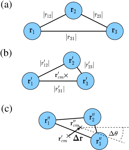
Figure 1: (a) The swimmer at time $t$. (b) The swimmer shape defined at time $t+\delta t$. The lengths of the two links connecting sphere $3$ have decreased. (c) The shape at $t+\delta t$ is translated by a vector $\Delta{\bf r}$ and rotated by an angle $\Delta\theta$ around its center of mass. These operations preserve the link lengths, thus leaving the shape unchanged. The parameters $\Delta{\bf r}$ and $\Delta\theta$ are chosen to improve upon the accuracy of the constraints in equation (3). This procedure is performed iteratively until the necessary accuracy is achieved.

The swimming motion is defined as a periodic shape change and, from this information, the algorithm must determine the trajectory of the swimmer through the fluid. To illustrate how this works we begin by considering a swimmer whose motion is confined to a two dimensional plane. Figure 1 shows the procedure for the case $N=3$. At a given time $t$, the position of the spheres ${\bf r}_{i}$ are known, as shown in figure 1(a). The new shape of the swimmer at the next time step $t+\delta t$ is shown in figure 1(b). We have chosen, for illustrative purposes, a swimming step where the lengths of the two links connecting sphere 3 have decreased.

The shape of the swimmer in figure 1(b) is defined through the three quantities $|r_{12}^{\prime}|$, $|r_{23}^{\prime}|$, and $|r_{31}^{\prime}|$. However, this information does not determine the absolute positions of the spheres. To find these, it is necessary to enforce the conservation conditions stated in equation (3). This is performed in the following iterative manner.

We take the first approximation for ${\bf r}_{i}(t+\delta t)$ to be ${\bf r}_{i}^{\prime}$. This does not, in general, obey equation (3), as will be apparent below. Our aim is to move the spheres in such a way as to successively improve the accuracy of equation (3). To do this, we consider translating the swimmer by a vector $\Delta{\bf r}=(\Delta x,\Delta y)^{T}$, and rotating it about its center of mass by an angle $\Delta\theta$, as illustrated in Figure 1(c). Note that these operations do not change the shape of the swimmer. In doing this, we introduce new position coordinates ${\bf r}_{i}^{\prime\prime}$ defined by

$${\bf r}_{i}^{\prime\prime}={\bf r}^{\prime}_{cm}+{\bf\Delta r}+{\bf R}\left({\bf r}^{\prime}_{i}-{\bf r}^{\prime}_{cm}\right)$$ (4)

where ${\bf R}$ is a clockwise rotation matrix around an angle $\Delta\theta$ and ${\bf r}^{\prime}_{cm}=\sum_{i=1}^{N}{\bf r}_{i}^{\prime}/N$ is the center of mass position of the swimmer. The unknown displacement ${\bf\Delta r}$ and angle $\Delta\theta$ are chosen to improve upon the accuracy of the constraints in equation (3). To calculate them we note that the velocity of sphere $i$ can be related to its displacement over time $\delta t$ by

$${\bf v}_{i} = \frac{{\bf r}_{i}^{\prime\prime}-{\bf r}_{i}}{\delta t}$$ (5)

$$\approx \frac{{\bf r}_{i}^{\prime}-{\bf r}_{i}+{\bf\Delta r}+\Delta\theta|{r}_{i}^{\prime}-{r}_{cm}^{\prime}|\hat{\bf r}_{i}^{\theta}}{\delta t}.$$

The unit vector $\hat{\bf r}_{i}^{\theta}$ lies in the direction a given point moves under an infinitesimal rotation (which can be calculated by rotating the vector ${\bf r}^{\prime}_{i}-{\bf r}^{\prime}_{cm}$ by $90^{o}$ clockwise and normalizing it).

Substituting expression (5) into equation (1), and numerically inverting the resulting matrix equation using Gaussian elimination, we obtain an expression for the forces acting on each sphere of the form

$${\bf F}_{i}={\bf a}_{i}+{\bf b}_{i}\Delta x+{\bf c}_{i}\Delta y+{\bf d}_{i}\Delta\theta$$ (6)

where ${\bf a}_{i}$, ${\bf b}_{i}$, ${\bf c}_{i}$, and ${\bf d}_{i}$ are constant vectors. Using this, the three constraints in equation (3) can, after some rearranging, be written

$${\bf A}\left(\begin{array}[]{c}\Delta x\\ \Delta y\\ \Delta\theta\end{array}\right)=\left(\begin{array}[]{c}e_{1}\\ e_{2}\\ e_{3}\end{array}\right),$$ (13)

where the matrix ${\bf A}$ and the column vector ${\bf e}$ are constants. Finally, this matrix equation can be inverted to obtain the values of $\Delta x$, $\Delta y$, and $\Delta\theta$ which are then used in equation (4) to obtain a better approximation, ${\bf r}^{\prime\prime}$, to the sphere positions at time $t+\delta t$. Repeating the procedure gives rapid convergence to the correct solution. Typically a single iteration improves the accuracy of equation (3) by a factor of $\sim 10$.

The approach is easily generalized to a swimmer moving in three dimensions. In this case there are three displacement parameters $\Delta x$, $\Delta y$, $\Delta z$, and three rotation parameters $\Delta\theta_{xy}$ $\Delta\theta_{yz}$, $\Delta\theta_{zx}$ (where, for example, $\Delta\theta_{xy}$ is a rotation in the $x$-$y$ plane). These six unknowns can be determined using the six constraints in equation (3). The method is the same as above, except equations (4-6) now contain the corresponding extra terms, and ${\bf A}$ in equation (13) becomes a six by six matrix.

The computation for one time step scales as $N^{3}$. For low to moderate values of $N$ the method is very fast. However, for $N\gtrsim 100$, it quickly becomes very computationally intensive.

II.2 Lattice-Boltzmann

The lattice Boltzmann algorithm is now a widely used mesoscopic modeling technique for simulating the behavior of complex fluids S01 ; Y06 . The method consists of an evolution equation for a mass density distribution function $f_{k}({\bf s},t)$, which can be considered as a simplified, discretized version of Boltzmann’s transport equation. The distribution function is defined at positions, ${\bf s}$, which lie on a cubic lattice with a distance $\delta s$ between nearest neighbor points. Its value is updated simultaneously and discretely in time, with time step $\delta t$. We define $c=\delta s/\delta t$. The subscript $k$ denotes a particular velocity direction ${\bf e}_{k}$. The velocity vectors ${\bf e}_{k}$ must be chosen such that ${\bf e}_{k}\delta t$ lies between lattice sites. In this study all simulations are performed in three dimension using a $15$ velocity model. This has a zero velocity vector ${\bf e}_{0}=(0,0,0)$, six nearest neighbor velocity vectors ${\bf e}_{1-6}$ in the directions $(\pm c,0,0)$, $(0,\pm c,0)$, and $(0,0,\pm c)$, and eight velocity vectors ${\bf e}_{7-14}$ in the diagonal directions $(\pm c,\pm c,\pm c)$. From $f_{k}$ we can calculate the mass density $\rho$ and momentum density $\rho{\bf u}$:

$$\rho=\sum_{k}f_{k}, \rho u_{\alpha}=\sum_{k}f_{k}e_{k\alpha}.$$ (14)

Evolution in time is given by

$$f_{k}({\bf s}+{\bf e}_{k}\delta t,t+\delta t)=f_{k}({\bf s},t)-\frac{1}{\tau}\Bigl{[}f_{k}({\bf s})-f_{k}^{eq}({\bf s})\Bigr{]}$$ (15)

where we use the Bhatnagar-Gross-Krook approximation, which uses a single parameter $\tau$ to determine the rate of relaxation toward equilibrium. A suitable choice for the equilibrium distribution function is

$$f^{eq}_{k} = \rho w_{k}\left(1+\frac{3e_{k\alpha}u_{\alpha}}{c^{2}}+\frac{9(e_{k\alpha}u_{\alpha})^{2}}{2c^{4}}-\frac{3u^{2}}{2c^{2}}\right)$$ (16)

where the weight factors are $w_{0}=\frac{2}{9}$, $w_{1-6}=\frac{1}{9}$, and $w_{7-14}=\frac{1}{72}$. Note that this distribution satisfies

$$\sum_{k}f_{k}^{eq}=\rho, \sum_{k}f_{k}^{eq}e_{k\alpha}=\rho u_{\alpha},$$ (17)

such that mass and momentum are conserved in time. This can be seen by summing the zeroth and first velocity moments of equation (15), and using the relations in (14).

Applying the Chapman-Enskog expansion to the lattice Boltzmann equation (15) Y06 gives the continuity equation for the total density,

$$\partial_{t}\rho+\partial_{\alpha}(\rho u_{\alpha})=0$$ (18)

and the Navier-Stokes equation for the fluid momentum,

$$\partial_{t}(\rho u_{\alpha})+\partial_{\beta}(\rho u_{\alpha}u_{\beta})=-\partial_{\alpha}\left(\rho c_{s}^{2}\right)+\partial_{\beta}\left(\nu\rho\partial_{\beta}u_{\alpha}\right)$$ (19)

where the kinematic viscosity is

$$\nu=\frac{(\delta s)^{2}}{3\delta t}\left(\tau-\frac{1}{2}\right)$$ (20)

and the speed of sound is $c_{s}=c/\sqrt{3}$. At low Reynolds numbers the fluid is, to a very good approximation, incompressible, i.e. $\nabla.{\bf u}=0$. (In the simulations, the difference between the maximum and minimum density within the system was found to be no more that $0.04\%$ of the average density.)

For simplicity, we do not explicitly consider a solid-fluid interface but define the swimmer to comprise of the fluid region within the spheres which make up the swimmer N3 . The swimmer-fluid interaction is incorporated into the lattice Boltzmann algorithm after finding the fluid velocities in equation (8), but before calculating the equilibrium distributions in equation (10). This interaction is generated in three stages. Firstly, the total linear and angular momentum of the swimmer are calculated:

$${\bf P}=\sum_{j}\rho_{j}{\bf u}_{j},\quad{\bf L}=\sum_{j}{\bf s}_{j}\times\rho_{j}{\bf u}_{j},$$ (21)

where the sum $j$ runs over all the lattice sites contained within the swimmer. Secondly, the new positions of the spheres are calculated. This procedure is analogous to that described for the Oseen tensor method in Section II.1. In this, we know the positions of the spheres at time $t$ and the swimmer shape at time $t+\delta t$. The algorithm works out how this new shape is oriented with respect to the original, such that linear and angular momentum are conserved, i.e.

$$\sum_{i}m_{i}{\bf v}_{i}={\bf P},\quad\sum_{i}{\bf r}_{i}\times m_{i}{\bf v}_{i}={\bf L},$$ (22)

where $m_{i}=\sum_{j}\rho_{j}$ and

$${\bf v}_{i}=\frac{{\bf r}_{i}(t+\delta t)-{\bf r}_{i}(t)}{\delta t}$$ (23)

are the mass and velocity of sphere $i$, respectively. Thirdly, the motion of the swimmer is coupled back to the fluid. Lattice sites within a given sphere are set to the velocity of that sphere, i.e. ${\bf u}_{j}={\bf v}_{i},\,\,\,{\bf s}_{j}\in\text{Sphere}\,\,i$. These updated velocities are then used in calculating the equilibrium distributions (16). Through repeated iteration of the lattice Boltzmann equation (9), the fluid within and immediately adjacent to the spheres is strongly coupled to move with the same velocity as the spheres, thus giving the correct boundary condition.

To avoid unwanted lattice effects, the radius $R$ of each sphere must be sufficiently large to accurately resolve its shape on the cubic grid. In this study we choose $R=3\delta s$, such that each sphere contains approximately $113$ lattice sites. Note that in this procedure we neglect the effect of rotation on the spheres, assuming that all parts of a given sphere travel at the same velocity. This assumption is justified because the hydrodynamic interactions between rotating spheres is rather weak. (The Oseen tensor (2) decays as $r^{-1}$, whereas the flow field around a rotating sphere decays at a much faster rate of $r^{-3}$.) In the case of modeling more than one swimmer, it is necessary to add hard core potentials between spheres to prevent them from overlapping.

II.3 Multiparticle Collision Dynamics

An alternative mesoscale approach, which solves the equations of fluctuating hydrodynamics is the multiparticle collision dynamics (also known as stochastic rotation dynamics) algorithm introduced by Malevanets and Kapral MK99 . The fluid is represented by a large number of point-like particles of mass $m$, with position $\mathbf{r}_{k}(t)$, and velocity $\mathbf{v}_{k}(t)$ at time $t$, where $k$ is the particle index. The particles move in continuous space, and at discrete time intervals, $\delta t$. Particle positions are updated according to

$$\mathbf{r}_{k}(t+\delta t)=\mathbf{r}_{k}(t)+\mathbf{v}_{k}(t)\delta t.$$ (24)

At each time step the particles also undergo a multiparticle collision that locally conserves mass, momentum, and energy. To perform the collision, the simulation box is divided into a grid of cubic cells, with sides of length $a$. The average number of particles per cell will be denoted by $\gamma$. The velocities of the particles in each cell are then rotated about the center of mass velocity of the cell, $\mathbf{v}_{cm}$

$$\mathbf{v}_{k}(t+\delta t)=\mathbf{v}_{cm}(t)+\mathbf{R}\left[\mathbf{v}_{k}(t)-\mathbf{v}_{cm}(t)\right].$$ (25)

$\mathbf{R}$ is a rotation matrix through a fixed angle, $\alpha$, about an axis that is generated randomly for each cell in the simulation at each time step. The position of the cubic grid is chosen randomly at each time step – this leads to substantially improved Galilean invariance in the algorithm IK01 . In the continuum limit, the multiparticle collision dynamics algorithm recovers the thermohydrodynamic equations of motion and thus acts as a Navier-Stokes solver. Conveniently, the dependence of the transport coefficients of the fluid on the simulation parameters is known analytically IK03 ; PY05 . Thus, it is a relatively simple task to choose values that result in a low Reynolds number fluid.

We couple a swimmer to the multiparticle collision dynamics solvent by considering it to be composed of a number of particles, and including these solute particles in the solvent collision step (25). In this way the swimming microstructure can exchange momentum with the solvent. In general, the equations of motion of the microstructure are solved using a velocity Verlet molecular dynamics algorithm. Precise details of how specific swimmers are dealt with using this approach are given in later sections of the paper.

III Linear Three Sphere Swimmer

Recently, Najafi and Golestanian NG04 proposed a one-dimensional swimmer comprising three connected spheres. Their model is perhaps the simplest example of a controlled, cyclic motion that breaks time reversibility. The swimmer consists of a central sphere that is connected to two other spheres by arms that are separated by an angle of $180^{o}$, are of negligible thickness, and whose length can be changed by, for example, the action of engines located on the central sphere. The microstructure moves by shortening and extending the lengths of the arms in a periodic and time irreversible manner, as shown in Figure 2. The relevant parameters for this model are $D$, the distance between the central sphere and an outer sphere at the maximum arm length, $\varepsilon$, the distance the arm shortens, $W$, the speed at which the arms change their lengths, and $R$, the radius of the spheres. The result of this cyclic, time irreversible motion is a net translation of the swimmer along the line linking the three spheres; we define $\Delta$ as the distance the swimmer translates in one complete cycle.

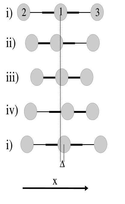
Figure 2: The four step, cyclic motion of the linear three sphere swimmer NG04 .

III.1 Analytic Theory

Because of the simplicity of the shape deformations of the linear three sphere swimmer, it is possible to calculate analytically the total net displacement, $\Delta$, of the swimmer during each complete cycle of its motion, in the limit of $\varepsilon\ll D$ and $R\ll D$. We summarize the argument of Najafi and Golestanian NG04 and correct their formula for the displacement of the swimmer, which we shall need for comparison to the numerical results.

Each of the four steps of the stroke can, by a simple transformation, be converted into one particular auxiliary stroke. In the auxiliary stroke one arm has a fixed length, $\delta$, where $\delta$ is either $D$ or $D-\varepsilon$, and the other arm changes length from $D$ to $D-\varepsilon$. We choose the x-axis to be parallel to the line linking the spheres and directed away from sphere $2$ (see Figure 2). During the auxiliary stroke $v_{1}=v_{3}$ and $W=v_{2}-v_{1}$, and thus the velocity of the middle sphere, in the limit that the swimmer undergoes small deformations, is

$$v_{1}(\delta) \approx\frac{-W\left(H_{11}-H_{23}-H_{12}\right)}{\left(3H_{11}-2\left(H_{12}+H_{13}+H_{23}\right)\right)}$$ (26)

$$\approx-\frac{W}{3}\left[1-\frac{R}{2(D-Wt)}+\frac{R}{\delta}-\frac{R}{2(\delta+D-Wt)}\right],$$

ignoring terms of order $(R/D)^{2}$ and greater. The elements of the Oseen tensor for each pair of spheres follow from equation (2). Integrating (26) gives the displacement over the auxiliary stroke,

$$\Delta_{a}(\delta)=\int^{\varepsilon/W}_{0}v_{1}(\delta)\,dt.$$ (27)

This can then be used to calculate the total displacement after the four step cycle, to second order in $\varepsilon/D$, as

$$\Delta = 2\left[\Delta_{a}(D)-\Delta_{a}(D-\varepsilon)\right]$$ (28)

$$= \frac{7}{12}R\left[\left(\frac{\varepsilon}{D}\right)^{2}+\left(\frac{\varepsilon}{D}\right)^{3}\right],$$

We note here that this expression differs from that given by Najafi and Golestanian NG04 who reported

$$\Delta=2.8R\left(\frac{\varepsilon}{D}\right)^{3}.$$ (29)

In equation (29) the displacement, $\Delta$, is proportional to $(\varepsilon/D)^{3}$. If one considers the transformation $\varepsilon\rightarrow\chi=-\varepsilon$ and $D\rightarrow G=D-\varepsilon$, this corresponds to a swimmer undergoing exactly the same continuous motion as that shown in Figure 2, only with the swimming stroke beginning at the third step in the cycle. Thus, the swimmer must move in the same direction. However, equation (29) suggests that the swimming direction is reversed under this transformation, which is clearly incorrect.

In the following section, we summarize the results of numerical simulation studies of the motion of the linear three sphere swimmer at low Reynolds number in order to validate and compare the use of these approaches in the study of swimming microstructures.

III.2 Numerical Results

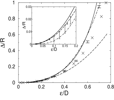
Figure 3: The shift per cycle of the linear three sphere swimmer, $\Delta$, as a function of the sphere displacement amplitude, $\varepsilon$. The inset shows a magnified view of the region of the graph below $\varepsilon/D=0.2$. The parameters $D=25$ and $R=3$ were used in the Oseen tensor and lattice Boltzmann approaches. In the multiparticle collision dynamics simulations we used $D=3.0a$. The solid line was obtained by numerically solving the Oseen tensor equation, outlined in section II.1. The crosses mark results obtained from lattice Boltzmann simulations, presented in section II.2. The error bars show the distribution of results using multiparticle collision dynamics from section II.3. The dashed line is the theoretical expression given in equation (28) and the dot-dashed line is the expression proposed by Najafi et al. NG04 reproduced in equation (29).

Figure 3 gives the results for a single linear three sphere swimmer, using each of the three methods presented in Section II. This graph shows how the total displacement of the swimmer over one swimming cycle, $\Delta$, varies as a function of the amplitude of the stroke, $\varepsilon$. The parameters used were $D=25$ and $R=3$ for the Oseen tensor and lattice Boltzmann approaches and $D=3.0a$ for the multiparticle collision dynamics simulations.

The solid line in Figure 3 is obtained by directly solving the Oseen tensor interaction between the spheres, as outlined in Section II.1. The dashed line shows the theoretical curve, equation (28), which is correct to third order in $\varepsilon/D$. These two curves converge in the limit of small $\varepsilon/D$, as expected. The dot-dashed line is equation (29), the expression proposed by Najafi and Golestanian NG04 . This appears to give good agreement for larger values of $\varepsilon/D$. This is misleading, however, as in the limit of small $\varepsilon/D$ it does not converge to the theoretical solution (this is seen most clearly within the inset), and it should not be valid at higher values of $\varepsilon/D$ due to the assumptions made in the derivation.

The lattice Boltzmann simulations were performed using a lattice of size $L_{x}=200$, $L_{y}=100$, and $L_{z}=100$, with periodic boundary conditions. Initially, the swimmer was placed in the middle of the box, aligned parallel to the $x$ direction. The relaxation parameter was chosen to be $\tau=1$. The simulations were run for one complete swimming cycle, which corresponded to $t_{max}=102400\delta t$ time steps. The maximum speed of spheres is approximated by $4\varepsilon/t_{max}$. Using this together with $R$, which gives a characteristic length scale for the problem, the Reynolds number can be expressed as $Re=4\varepsilon R/\nu t_{max}$. The largest displacement used ($\varepsilon=19$) gives $Re=0.013$. This was checked to be sufficiently low by running a limited number of simulations using $t_{max}=204800\delta t$ time steps, and finding that these results agreed to within $1\%$. Furthermore, we checked that finite size effects were not important by performing simulations using a lattice of size $L_{x}=300$, $L_{y}=150$, and $L_{z}=150$, with results again agreeing within this tolerance.

The results from the lattice Boltzmann simulations are denoted by the crosses in Figure 3. They agree well with the full Oseen tensor result (solid curve) at small $\varepsilon/D$ and deviate as $\varepsilon/D$ gets increasingly large. This is because the Oseen tensor approximation that the spheres are far apart breaks down in this limit (the spheres intersect each other if $\varepsilon/D>0.76$ for the parameters used).

Simulations using multiparticle collision dynamics are intrinsically noisy. If we simply use a molecular dynamics algorithm to solve the equations of motion for the swimmer and include the particles that make up the swimmer in the solvent collision step then, without further correction, the microstructure will rotate, and not stay aligned along one particular axis. Although this behavior would be realistic for a nanoscale microstructure in a solvent, it does not easily allow for an accurate comparison of swimming speed with theory. To constrain the motion to one dimension, the transverse velocities of the three particles that comprise the swimmer were adjusted to the average velocity of the particles after each collision step. Changes in the arm lengths were undertaken by adding an extra velocity to each particle, such that the total momentum of the microstructure remained unchanged during the arm length change.

For the multiparticle collision dynamics solvent we used the following parameters: Particle temperature $kT=0.005$, time step $\delta t=0.01$, cell size $a=1.0$, rotation angle $\alpha=135^{o}$, average number of particles per cell $\gamma=10$, and particle mass $m=10$. These result in a Reynolds number for the microstructure of $\sim 10^{-5}$. These parameters both ensure a low Reynolds number and minimize fluctuations in the solvent with a high Schmidt number. In our simulations, we employed a simulation box of dimensions $30a\times 8a\times 8a$ with periodic boundary conditions and checked for finite size effects. For the swimmer we used a mass of $5m$ for each sphere. Due to the nature of the swimmer–solvent interaction in our implementation of the multiparticle collision dynamics algorithm, it is difficult to define the effective hydrodynamic radii of the spheres. However, comparison with the Oseen tensor and lattice Boltzmann simulation results suggests the parameters used lead to $R/D\sim 0.12$. The simulations were conducted for a total time of $t_{max}=2.72\times 10^{5}\delta t$ time steps, and one period of motion took $6.8\times 10^{3}\delta t$. The period must be sufficiently long to allow the solvent to couple with the swimmer. 20 runs were performed for each parameter set and the results are denoted by the error bars in Figure 3, which are spread one standard error on either side of the average of the 20 runs. The results are compatible with, but much less precise than, those obtained by the methods without intrinsic fluctuations.

Figure 4: The percentage efficiency of a linear three sphere swimmer as a function of (a) the sphere displacement amplitude, $\varepsilon$, for fixed $D=5R$, and (b) the maximum arm length, $D$, for fixed minimum separation $D-\varepsilon=4R$.

By changing the parameters, $D$ and $\varepsilon$, it is not only possible to change the swimmer displacement, $\Delta$, but also the efficiency of the swimmer. We define this efficiency to be the energy required for an external force to move the individual spheres by the distance $\Delta$ in a time $P$ divided by the work done by the swimmer in performing the corresponding cyclic shape change:

$$\text{Efficiency}=\frac{6\pi\eta N\Delta^{2}/P}{\sum_{i=1}^{N}\int_{0}^{P}\mathbf{F}_{i}.\mathbf{v}_{i}dt}.$$ (30)

Using the Oseen tensor approach, the forces on the spheres, $\mathbf{F}_{i}$, are calculated through equation (6), so this quantity is easily obtainable. The line in figure 4(a) shows how the swimming efficiency is changed as a function of $\varepsilon$, whilst keeping $D=5R$ fixed. Note that this curve terminates when $\varepsilon=D-2R$, since beyond this the spheres unphysically overlap at some point within the swimming cycle. Furthermore, the Oseen tensor method tends to overestimate the efficiency when the spheres get close, because it does not include the viscous dissipation resulting from lubrication effects. Figure 4(a) illustrates a general feature of swimmers, namely that small amplitude motion results in inefficient swimming. The curve in figure 4(b) shows the efficiency against $D$, assuming a fixed mimumum sphere separation of $D-\varepsilon=4R$. We find that the swimmer becomes increasingly efficient as $D$ increases, approaching a limit of around $8\%$.

We now summarize the relative advantages and disadvantages of the three numerical methods. The Oseen tensor approach is particularly advantageous for swimmers comprising small numbers of spheres because it is computationally very fast (simulations taking only minutes instead of days using lattice Boltzmann or multiparticle collision dynamics). This is primarily because it is not necessary to explicitly solve a set of fluid dynamics equations. However the simulation time scales as $N^{3}$ so lattice Boltzmann becomes more efficient for large numbers of swimmers.

The Oseen tensor formalism is also limited because it assumes that the interacting spheres are spaced far apart, compared to their radii. This means, for instance, that it would not be appropriate to use this method to study the movement of a swimmer close to a wall or in a confined geometry. On the other hand, the lattice Boltzmann algorithm can address these problems, providing an exact solution to any fluid flow problem given sufficient resolution. In practice it is limited by computational power. To avoid spurious lattice effects, the sphere radius must be significantly larger than the lattice size, necessitating the need for large systems. Moreover, to obtain a sufficiently low Reynolds number, the cyclic swimming motion must be performed over a great number of time steps, further increasing the computational burden.

Multiparticle collision dynamics is advantageous because it is unconditionally stable, unlike the lattice Boltzmann method, and this allows somewhat lower Reynolds numbers to be obtained more easily. One can also use a molecular dynamics approach to treat the microstructure allowing for great flexibility in the swimmer models it is possible to consider.

Additionally, as this method inherently contains noise it will be appropriate for studying very small scale structures, for which Brownian fluctuations are important. However, if the fluctuations are unphysical the noise is undesirable, necessitating long time averages.

For the remainder of this paper, we concentrate on using the Oseen tensor and multiparticle collision dynamics approaches to study more complex swimming motions.

IV Generalized Three Sphere Swimmers

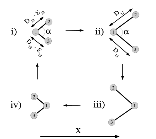
Figure 5: Alternative cyclic motion for a three sphere swimmer, allowing the microstructure to translate in two dimensions. Possible extensions to this scheme include allowing the angle $\alpha$ to change as the arm lengths change.

The swimmer described in Section III is constrained to move in one dimension along its axis. Using the same basic elements one can design a number of other three sphere swimmers that can move their individual components and centers of mass in two or three dimensions. To extend the original design we allow the angle between the two arms of the swimmer to change DB05b . When the change in angle takes place, the spheres may move radially with the arm lengths constant, or the arm lengths may change at the same time, thus allowing for a number of different motions. In Figure 5 we show one of many possible alternative schemes of motion for swimmers of this type, which we will refer to as generalized three sphere swimmers.

Figure 6: The position shift over one cycle, $\Delta$, as a function of swimmer angle $\alpha$ for the swimmer defined in Figure 5. Other parameters were $D=5R$ and $\varepsilon=2R$.

We first concentrate on the motion shown in Figure 5, and the case where the arms rotate at fixed length. If the swimmer employs a symmetric motion with arm lengths $D_{12}=D_{13}$ and $\varepsilon_{12}=\varepsilon_{13}$, the net translation of the swimmer is along the x-axis (defined in the figure). Thus, the microstructure remains a one dimensional swimmer while its individual elements are moving in two dimensions. Interestingly, the direction that the microstructure translates varies with $\alpha$, for fixed $D$ and $\varepsilon$, as shown in Figure 6. For $D=5R$ and $\varepsilon=2R$ the outer two spheres do not intersect for $\alpha>39^{o}$, and there is a transition from backward motion to forward motion at $\alpha=77^{o}$. Intuitively it is not obvious what causes this reversal of direction. We found that the maximum efficiency of this swimmer (with efficiency defined by equation (30)), occurs at $\alpha=138^{o}$. This corresponds to an efficiency of $1.8\%$, which is considerably less than the $\sim 8\%$ found for the linear three sphere swimmer in the previous section. It seems plausible that the linear three sphere swimmer is the most efficient three sphere swimmer possible.

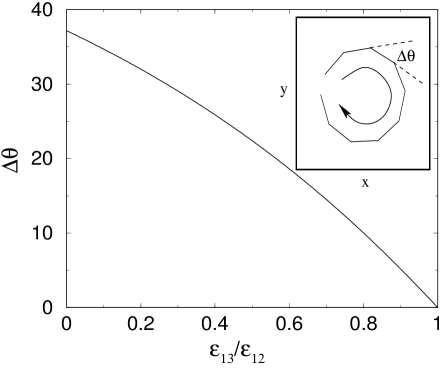
Figure 7: The angular change in the orientation of the generalized three sphere swimmer over one complete swimming cycle, $\Delta\theta$, as a function of the swimmer displacement amplitude, $\varepsilon_{13}$. Other parameters were fixed to be $\varepsilon_{12}=3R$ and $D_{12}=D_{13}=6R$. The inset shows the movement of the center of mass of the swimmer at a fixed point in the cycle, over the course of 9 swimming cycles.

If one instead defines an asymmetric motion, with $D_{12}\neq D_{13}$ and/or $\varepsilon_{12}\neq\varepsilon_{13}$, the microstructure will move its center of mass in two dimensions. The swimmer rotates and translates, as shown for $D_{12}=D_{13}=6$, $\varepsilon_{12}=3$ and $\varepsilon_{13}$ as variable in Figure 7. As the difference between $\varepsilon_{12}$ and $\varepsilon_{13}$ becomes greater, the angular rotation about the center of mass of the microstructure for each swimming cycle increases. Thus, it is a relatively easy step to imagine a manufactured device that can switch between symmetric and asymmetric cyclic motions, perhaps in response to an external stimulus or experimental condition, to enable movement in a controlled fashion in two dimensions. A three sphere swimmer, that can change the angle between its two arms, could simply adopt the efficient swimming motion of Section III, where $\alpha=180^{o}$, to move in a straight line, and then vary $\alpha$ to adopt a structure allowing it to turn.

To extend the movement of such a microstructure to three dimensions, the angle between the arms could be changed along another plane, perpendicular to the original one. One strategy to do this might be to employ a double-jointed structure where the angle between the arms could be changed from $\alpha=180^{o}$ in either of two perpendicular planes. It is of interest that this microstructure is the first low Reynolds number swimmer to be proposed theoretically that can move in a controlled fashion in three dimensions, without employing numerous one dimensional swimming devices placed perpendicular to each other.

V Extended, Linear, One Dimensional Swimmers

To extend the linear three sphere swimmer of Section III one can simply add more spheres to the microstructure, the simplest extension being the four sphere case. For the four sphere microstructure shown in Figure 8i), we analyzed through Oseen tensor based numerical simulations all possible cyclic motions that are made up of a discrete number of steps. At the end of each step the distance between neighboring spheres is either $D$ (an extended rod) or $D-\varepsilon$ (a contracted rod). If a rod changes length during a step then it does so at a constant speed $W$. In this analysis we allowed for more than one rod length changing simultaneously.

Out of this subset of possible swimmers the swimming strategy shown in Figure 8 is the most efficient. This optimal swimming strategy proceeds as follows: Starting from the fully extended conformation, i), the distance between spheres $1$ and $2$ is reduced to $D-\varepsilon$, ii). In the next two steps the distance between spheres $2$ and $3$ is reduced to $D-\varepsilon$, iii), and the distance between spheres $3$ and $4$ is reduced to $D-\varepsilon$, iv), the fully contracted conformation. The microstructure then sequentially extends, first by extending the distance between spheres $1$ and $2$ to $D$, v), then extending the distance between spheres $2$ and $3$ to $D$, vi), and finally by extending the distance between spheres $3$ and $4$ to $D$, completing the cycle and taking the conformation back to the original starting configuration i). For the case $D=5R$ and $\varepsilon=2R$, the four sphere microstructure using the optimal swimming strategy has a swimming efficiency of 6.9 % compared to 4.5 % for the three sphere swimmer using the same parameters.

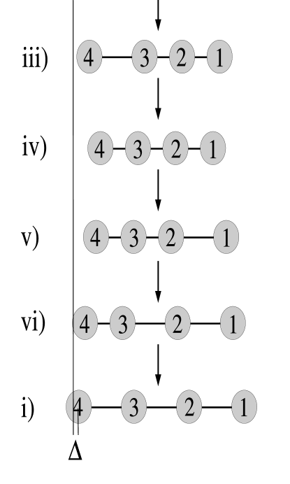
Figure 8: The most efficient cyclic swimming strategy for an extended, linear, four sphere microstructure.

Extending to the five sphere case, we analyzed all possible cyclic swimming strategies using Oseen tensor based numerical simulations, and found that the analogous swimming strategy to that in Figure 8 was optimal, resulting in a swimming efficiency of 8.8 % for the $D=5R$ and $\varepsilon=2R$ case. We studied this optimal swimming strategy for microstructures with up to 200 spheres and the swimming efficiency as a function of the number of spheres is shown in Figure 9.

Figure 9: Percentage efficiency against the number of spheres for a microstructure adopting the swimming strategy depicted in Figure 8.

The curve indicates a logarithmic growth in the efficiency as a function of sphere number. This would imply that for a sufficiently large number of spheres the efficiency will go above one. Although counter intuitive, from our definition of efficiency in equation (30), this is perfectly possible, and does not violate any physical principles. However, as the number of spheres is increased, the physical size of the spheres and rods would have to be made proportionately smaller, to ensure that finite Reynolds number effects do not become important.

VI Filament Swimmers Using Multiparticle Collision Dynamics

As an example of using multiparticle collision dynamics to investigate a more complicated swimmer we consider the motion of a filament modeled as beads connected by springs and interacting through Lennard-Jones forces. The filament is driven by a sinusoidally oscillating force applied at one end. The model was motivated by the man-made microscopic swimmer of Dreyfus et al. where a red blood cell is attached to a filament consisting of superparamagnetic colloids, that are connected to each other using DNA DB05a . Two magnetic fields are used experimentally, one to align the filament and the other to actuate one end of it in a sinusoidal manner. This actuation results in a series of waves, originating at the tail of the filament, propagating towards the red blood cell at the head. Because the perpendicular and parallel friction coefficients of the microstructure are not equal ($\zeta_{\perp}/\zeta_{\parallel}\approx 2$), a net translation, in the opposite direction to the propagation of the wave, occurs along the alignment direction of the filament.

In the multiparticle collision dynamics simulation we model the filament as a number of Lennard-Jones beads, representing the superparamagnetic colloids, connected to each other by FENE springs, representing the DNA linkers. Instead of a magnetic field, we simply apply an equal and opposite force to each end of the filament to align it along an axis, and apply a sinusoidal actuating force, perpendicular to the aligning forces, to one end of the filament (see Figure 10(a)).

Lowe L01 proposed a dimensionless parameter to characterize naturally flexible filaments, the ‘sperm number’, defined as

$$S_{p}=L/\left(\frac{\kappa}{\zeta_{\perp}\omega}\right)^{1/4}$$ (31)

where $L$ is the length, $\kappa$ is the bending rigidity, and $\zeta_{\perp}$ is the perpendicular friction coefficient for the filament, and $\omega$ is the angular frequency of the actuation or driving. For our model filament in a multiparticle collision dynamics solvent we calculate the bending rigidity from the change in energy of the structure as a function of the curvature of the filament LC03 . We determine the friction coefficients by applying a known force to each bead, in a direction perpendicular or parallel to the alignment, and measuring the resulting velocity of the microstructure (with no actuation). We can then measure how the velocity of the microstructure depends on $S_{p}$ by changing the angular frequency of the actuation.

For the multiparticle collision dynamics solvent we use the following parameters: $kT=1.0$, $\delta t=1.0$, $a=1.0$, $\alpha=120^{o}$, $\gamma=5$, and $m=4$ resulting in a Reynolds number for the microstructure of $\sim 10^{-2}$. For the microstructure we use a mass of $4m$ for each bead and a molecular dynamics time step of $0.002\delta t$. The average distance between the centers of mass of each bead is $\approx 1.0a$, and we use 10 beads to represent the filament. The simulations are conducted over $t_{max}=200000\delta t$ solvent time steps, and we average the results over 10 runs for each data point.

In Figure 10 we show the swimming velocity of the microstructure, scaled by $L\omega$, as a function of $S_{p}$. As predicted by theory for naturally flexible filaments WG98 , we observe a maximum in the scaled swimming velocity of the filament between the high (dominated by viscous friction) and low (dominated by internal elasticity) $S_{p}$ regimes. This reproduces the behavior demonstrated for the man-made swimmer of Dreyfus et al. DB05a , and we also observe very similar scaled speeds in our simulations to those found experimentally.

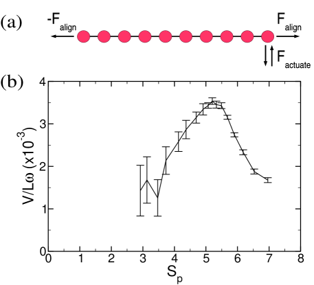
Figure 10: (a) Model filament used in the multiparticle collision dynamics simulations. The filament is composed of Lennard-Jones beads that are connected by FENE springs. An aligning force, $F_{align}$, is applied to both ends of the filament, and a sinusoidal force, $F_{actuate}=F_{max}\sin(\omega t)$, is used to actuate one end of the microstructure, leading to wave propagation from right to left in the diagram. (b) Scaled swimming velocity as a function of the sperm number for the flexible filament. To obtain this plot, $F_{max}$ is varied for different frequencies of actuation such that the integral of $F_{actuate}$ over half of the period is equal.

To verify that the filament in the simulations swims through the mechanism of wave propagation, we also modeled a 2 bead microstructure under the influence of aligning and actuating forces. We find that this microstructure does not swim as it is impossible for a 2 bead filament to move in a time irreversible fashion.

VII Conclusions

In this paper we have described three different methods for simulating low Reynolds number swimmers: An Oseen tensor approach, lattice Boltzmann and multiparticle collision dynamics. In Section III, each of these methods was used to model a very simple, linear swimmer comprising three linked spheres. Analytic results are available for this system NG04 and hence we were able to validate the approaches and identify the strengths and weaknesses of each method. For swimmers made up of a small number of spheres the Oseen tensor approach is very fast. However as the number of spheres increases, or as multiple swimmers are considered, lattice Boltzmann becomes more efficient. Moreover the Oseen tensor does not accurately take into account short range hydrodynamic interactions. Lattice Boltzmann is able to deal with spheres close to each other or to a surface, but at the expense of an increasingly fine lattice resolution. We found that multiparticle collision dynamics is in general a less useful approach as the intrinsic noise tends to dominate the results. This method will be of use when modeling nanoscale systems where fluctuations are an intrinsic component of the physics.

Subsequently, in Section IV, we proposed a new three sphere swimmer, which has the advantage of being able to turn, and control its trajectory in a three dimensional manner. These ideas may be of use in the design and fabrication of artificial microswimmers. Section V extended the one dimensional three sphere swimmer aiming to search for the most efficient swimming strategy for a larger number of spheres. We found that the efficiency increases logarithmically with the sphere number.

In Section VI, we looked at modeling a filament swimmer that moves due to the propagation of waves along its length. Using multiparticle collisional dynamics we were able to reproduce the behavior observed experimentally.

There are many directions in which it would be fruitful to pursue the simulations. We are currently considering interactions between two or more swimmers, and it would be of interest to consider the effect of boundaries and obstacles on swimming behavior. Continuum hydrodynamic theories have recently been proposed to describe concentrated solutions of swimmers SR02 ; LM05 . These have led to results very suggestive of swimming behavior but it is hard to pin down the phenomenological parameters in the equations of motion. Simulations of increasing numbers of swimmers are needed to try to bridge the gap between the microscopic and continuum approaches.

There is enormous scope presented by more realistic biological problems such as the chemotactic responses of bacteria or random tumbling during a swimming cycle. Moreover simulations of this type may be important in designing artificial microswimmers for applications as diverse as drug delivery or mixing fluids within microchannels.

References

- (1) R. Dreyfus, J. Baudry, M. L. Roper, M. Fermigier, H. A. Stone, and J. Bibette, Nature 437 862 (2005).
- (2) The dimensionless Reynolds number is defined by , where is a characteristic velocity, is a characteristic length, and is the kinematic viscosity of the fluid. It is clear that since for a typical liquid, then on the micron scale .
- (3) E. M. Purcell, Am. J. Phys. 45 3 (1977).
- (4) A. Shapere and F. Wilczek, J. Fluid Mech. 198 557 (1989); ibid. 198 587 (1989).
- (5) J. E. Avron, O. Kenneth, and D. H. Oaknin, New. J. Phys. 7 234 (2005).
- (6) R. Dreyfus, J. Baudry, and H. A. Stone, Euro. Phys. J. B 47 161 (2005).
- (7) A. Najafi and R. Golestanian, Phys. Rev. E 69 062901 (2004).
- (8) L. E. Becker, S. A. Koehler, and H. A. Stone, J. Fluid Mech. 490 15 (2003).
- (9) B. U. Felderhof, Phys. Fluids 18 063101 (2006).
- (10) E. Gauger and H. Stark, Phys. Rev. E 74 021907 (2006).
- (11) E. Yariv, J. Fluid Mech. 550 139 (2006).
- (12) H. A. Stone and A. D. T. Samuel, Phys. Rev. Lett. 77 4102 (1996).
- (13) C. M. Pooley and A. C. Balazs, submitted to Phys. Rev. E.
- (14) R. Golestanian, T. B. Liverpool, and A. Ajdari, Phys. Rev. Lett. 94 220801 (2005).
- (15) C. Dombrowski, L. Cisneros, S. Chatkaew, R. E. Goldstein, and J. O. Kessler, Phys. Rev. Lett. 93 098103 (2004).
- (16) E. Lauga, W. R. DiLuzio, G. M. Whitesides, and H. A. Stone, Biophys. J. 90 400 (2006).
- (17) L. Cisneros, C. Dombrowski, R. E. Goldstein, and J. O. Kessler, Phys. Rev. E 73 030901(R) (2006).
- (18) C. Beta, private communication.
- (19) J. P. Hernandez-Ortiz, C. G. Stoltz, and M. D. Graham, Phys. Rev. Lett. 95 204501 (2005).
- (20) S. Ramachandran, S. Kumar, and I. Pagonabarraga, Eur. Phys. J. E 20 151 (2006).
- (21) C. P. Lowe, Phil. Trans. R. Soc. London B 358 1543 (2003).
- (22) M. C. Lagomarsino, F. Capuani, and C. P. Lowe, J. Theo. Biol. 224 215 (2003).
- (23) L. D. Landau and E. M. Lifshitz, Fluid mechanics, Pergamon, Oxford (1987).
- (24) J. M. Yeomans, Physica A 369 159 (2006).
- (25) S. Succi, The lattice Boltzmann equation for fluid dynamics and beyond, Clarendon Press, Oxford (2001).
- (26) A. Malevanets and R. Kapral, J. Chem. Phys. 110 8605 (1999).
- (27) This can be seen by rearranging the small Reynolds number condition to give , i.e. the time taken for momentum to diffuse a distance is much smaller than the time for the sphere to move that same distance.
- (28) Since within this framework the interior of the spheres is essentially fluid, we lose the freedom to choose the mass density of the swimmer. However, for the simulations performed here, in which the Reynolds number is very low, inertial effects are unimportant. Therefore, this condition is not restrictive.
- (29) T. Ihle and D. M. Kroll, Phys. Rev. E 63 020201 (2001).
- (30) T. Ihle and D. M. Kroll, Phys. Rev. E 67 066705 (2003); ibid. 67 066706 (2003).
- (31) C. M. Pooley and J. M. Yeomans, J. Phys. Chem. B 109 6505 (2005).
- (32) C. P. Lowe, Fut. Gen. Comp. Sys. 17 853 (2001).
- (33) C. H. Wiggins and R. E. Goldstein, Phys. Rev. Lett. 80 3879 (1998).
- (34) R.A. Simha and S. Ramaswamy, Phys. Rev. Lett. 89 058101 (2002).
- (35) T.B. Liverpool and M. C. Marchetti, Europhys. Lett. 69 846 (2005).