Rashba quantum wire: exact solution and ballistic transport

Abstract

The effect of Rashba spin-orbit interaction in quantum wires with hard-wall boundaries is discussed. The exact wave function and eigenvalue equation are worked out pointing out the mixing between the spin and spatial parts. The spectral properties are also studied within the perturbation theory with respect to the strength of the spin-orbit interaction and diagonalization procedure. A comparison is done with the results of a simple model, the two-band model, that takes account only of the first two sub-bands of the wire. Finally, the transport properties within the ballistic regime are analytically calculated for the two-band model and through a tight-binding Green function for the entire system. Single and double interfaces separating regions with different strengths of spin-orbit interaction are analyzed injecting carriers into the first and the second sub-band. It is shown that in the case of a single interface the spin polarization in the Rashba region is different from zero, and in the case of two interfaces the spin polarization shows oscillations due to spin selective bound states.

1 Introduction

The Spintronics [1] is one of the most prominent fields of modern condensed matter physics. Its target is to use spin to create electrical and optoelectronic devices with new functionalities [2]. Up to now, starting form the seminal device by Datta and Das [3], several devices based on the giant and tunnel magnetoresistance have been realized for read-head sensors and magnetic random-access memories [2]. The important task of the integration of such spintronics technologies with the classical semiconductor devices finds an obstacle in the small spin injection from magnetic to semiconductor materials due to the large resistivity mismatch between magnetic and semiconductor materials [4]. For this reason it is useful to design semiconductor devices with an efficient all-electrical spin-injection and detection via Ohmic contacts at the Fermi energy, as it has been already realized for metallic devices [5, 6].

Two important classes of spin-orbit interaction (SOI) are relevant for semiconductor spintronics: the Dresselhaus type [7] and the Rashba type [8] coupling. The former arises from the lack of symmetry in the bulk inversion whereas the latter arises from the asymmetry along the growing-direction-axis of the confining quantum well electric potential that creates a two-dimensional electron gas (2DEG) on a narrow-gap semiconductor surface. Since the Rashba SOI can be tuned by an external gate electrode [9, 10, 11] it is envisaged as a tool to control the precession of the electron spin in the Datta-Das proposal for a field-effect spin transistor [3].

Quasi-one-dimensional electron gases or quantum wires (QWs) are realized by applying split gates on top of a 2DEG in a semiconductor heterostructure [12]. The main effect owing to the confining potential is quantization of the electron motion in the direction orthogonal to the wire axis. The combination of this confining potential and the Rashba SOI gives rise to sub-band hybridization that can affect the working principle of the field-effect spin transistor. Mireles and Kirczenow [13] have numerically studied this effect and they have shown that a large value of the Rashba SOI can produce dramatic changes in the transport properties of the device till to suppress the expected spin modulation. The effect of sub-band hybridization has been investigated by Governale and Züelike [14] in a QW with parabolic confinement. They show that electrons with large wave vectors in the lowest spin-spit sub-bands have essentially parallel spin. But in proximity of the anti-crossing points due to the sub-band hybridization it is no more appropriate to use the spin quantum number in order to characterize the electron state in the QW. Furthermore, they show that it is not possible to transfer the finite spin polarization of the QW to some external leads.

In this Article we study the spectral and the transport properties of a QW in the presence of SOI. The main result of this Article is to show how to achieve non-zero spin polarization in external leads using spin unpolarized injected carriers. This can be obtained by injecting carriers in all the active sub-bands due to the quantum confinement. At the opening of each new sub-band the hybridization owing to SOI gives rise to spin selective bound states reflecting in a oscillating spin polarization. Here, we want to stress that those spin polarized bound states are not in contradiction with any fundamental symmetry property of the system [15].

This Article is organized in the following way: in Sec. 2 we evaluate the spectral properties using the wave function approach [16, 17, 18]. In Sec. 3 we provide an exact calculation for the spectral properties investigated within the perturbation theory approach and with the exact diagonalization in a truncated Hilbert space. Here we also introduce a minimal model featuring the basic characteristic of a QW with SOI named two-band model. This is used in Sec. 4 in order to study the transport properties of a QW in presence of a single interface between a region with and without SOI and in the case of a double interface (spin-field effect transistor scheme). Conclusions are ending the Article.

2 Exact solution of Rashba quantum wire: wave-function 

Let us consider a 2DEG filling the plane ($x,z$). The charge carriers have momentum $\vec{p}\equiv(p_{x},p_{z})$ and effective mass $m$. The particles are confined along the $z$-direction by the potential $V(z)$ and subjected to the Rashba spin-orbit interaction (SOI). The single-particle Hamiltonian reads

$$\mathcal{H}=\frac{1}{2m}\left(p_{x}^{2}+p_{z}^{2}\right)+V(z)+\mathcal{H}_{\mathrm{R}},$$ (1)

where $\mathcal{H}_{\mathrm{R}}$ is the Rashba SOI

$$\mathcal{H}_{\mathrm{R}}=\frac{\hbar k_{\mathrm{SO}}}{m}\left(\sigma_{z}p_{x}-\sigma_{x}p_{z}\right).$$ (2)

In Eq.(2) $\sigma_{x}$ and $\sigma_{z}$ are the $x$ and $z$ components, respectively, of the vector $\vec{\sigma}$ of Pauli matrices, and $k_{\mathrm{SO}}$ is the SOI constant. This can be tuned by means of external gates perpendicular to the 2DEG [9, 10, 11].

In the following we assume that the potential $V(z)$ provides a confinement with hard walls at $z=0$ and $z=W$. The strategy to find the wave-function of the Hamiltonian (1) is similar to the procedure followed in the absence of SOI: one exactly solves the 2D problem, then considers the quantizing effect of confinement on the wave function $\psi(x,z)$. In the first subsection we shortly recall the spin-dependent solution of the 2DEG with SOI, then we impose the boundary conditions $\psi(x,z=0)=\psi(x,z=W)=0$. In the presence of SOI, these relations mix the $z$ part of the wave-function with its spinor component.

2.1 Solution without confinement

Without confinement both components of the momentum $\vec{p}=\hbar\vec{k}$ are conserved. The eigenfunctions of the Hamiltonian (1) in the absence of confining potential $V(z)=0$ are denoted by the two spin modes $(+)$ and $(-)$ and read

$$\psi_{\vec{k},+}\left(x,z\right) = \exp\left[\mathrm{i}(k_{x}x+k_{z}z)\right]\left(\begin{array}[]{c}\cos(\theta/2)\\ -\sin(\theta/2)\end{array}\right),$$ (3c)

$$\psi_{\vec{k},-}\left(x,z\right) = \exp\left[\mathrm{i}(k_{x}x+k_{z}z)\right]\left(\begin{array}[]{c}\sin(\theta/2)\\ \cos(\theta/2)\end{array}\right),$$ (3f)

whose corresponding eigenvalues are given by

$$E_{\pm}=\frac{\hbar^{2}}{2m}\left(k^{2}\pm 2kk_{\mathrm{SO}}\right),$$ (3d)

where $k=\sqrt{k_{x}^{2}+k_{z}^{2}}$ is the modulus of the wave-vector in $x$-$z$ plane, $k_{x}=k\cos(\theta)$, $k_{z}=k\sin(\theta)$, with $\theta$ the angle formed between the vector $\vec{k}$ and the $x$ axis. It is clear for Eqs. (3c,3f) that the spinors $\chi_{\pm}$ of the two modes are orthogonal to each other. We remind that the Rashba SOI can be viewed as a magnetic field parallel to the ($x,z$) plane and orthogonal to the wave-vector $\vec{k}$. The net effect is to orientate the spin along the direction perpendicular to the wave-vector [16].

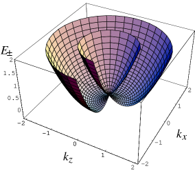
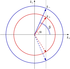
Figure 1: (Left Panel) Spectrum of the two-dimensional electron gas in the presence of SOI interaction as a function of the wave-vectors $k_{x}$ and $k_{y}$. At fixed positive energy, the wave-vectors of the mode $(+)$ and $(-)$ are on two concentric circles (radius for $(-)$ mode larger than that for the $(+)$ mode).(Right Panel) At fixed positive energy and x component of the wave-vector, the 4 possible values of the z component are shown.

In order to determine the solution with confinement, it is essential to find the eigenfunctions in the free case when the total energy $E$ and the momentum along $k_{x}$ are fixed (See Fig. 1). Fixing the total energy $E$ , we note that there are two values of total momentum $k$, corresponding to the different modes, fulfilling the Eq. (3d) expressed as a linear combination of those four waves:

$$k_{\pm}=\sqrt{\frac{2m}{\hbar^{2}}E+k_{\mathrm{SO}}^{2}}\mp k_{\mathrm{SO}}.$$ (3e)

The propagation directions for the $k_{\pm}$ modes are fixed by the momentum $k_{x}$. For $E>0$, the mode ($+$) is characterized by the propagation direction $\pm\alpha=\arccos(k_{x}/k_{+})$ fixing the value of $k_{z}=\pm k_{+}\sin(\alpha)$, whereas the mode ($-$) has propagation direction $\pm\beta=\arccos(k_{x}/p_{-})$ and $k_{z}=\pm k_{-}\sin(\beta)$. Therefore, the generic wave function $\psi_{E,k_{x}}(x,z)$ is given by

$$\psi_{E,k_{x}}\left(x,z\right)=\rme^{\mathrm{i}k_{x}x}\left[A\psi_{1,E}^{(+)}(z)+B\psi_{2,E}^{(+)}(z)+C\psi_{1,E}^{(-)}(z)+D\psi_{2,E}^{(-)}(z)\right],$$ (3f)

with

$$\psi_{\ell,E}^{(+)}(z)=\rme^{-\mathrm{i}(-1)^{\ell}k_{+}z\sin(\alpha)}\left(\begin{array}[]{c}\cos(\alpha/2)\\ (-1)^{\ell}\sin(\alpha/2)\end{array}\right),$$ (3g)

$$\psi_{\ell,E}^{(-)}(z)=\rme^{-\mathrm{i}(-1)^{\ell}k_{-}z\sin(\beta)}\left(\begin{array}[]{c}-(-1)^{\ell}\sin(\beta/2)\\ \cos(\beta/2)\end{array}\right),$$ (3h)

and $\ell=1,2$.

For $-k_{-}\leq k_{x}<-k_{+}$ or $k_{+}<k_{x}\leq k_{-}$, the wave-function (3f) is still valid. However, one has $\alpha=\mathrm{i}a$, implying that $\cos(\alpha)=\cosh(a)$ and $\sin(\alpha)=\mathrm{i}\sinh(a)$, therefore the ($+$) mode becomes an evanescent one. Moreover, if $k_{x}>k_{-}$ or $k_{x}<-k_{-}$, then $\beta=\mathrm{i}b$ and also the ($-$) mode changes into an evanescent one.

For $E<0$ the 4 values of $k_{z}$ are only relative to modes $(-)$. A wave-function similar to (3f) can be written. Also in this case the Fermi surface is formed by two circles but now they correspond to the same energy $E_{-}$. However, in the next section, we will see that, from weak to intermediate values of the Rashba SO coupling, only positive values of the energy are important due to the effect of the confinement.

2.2 Solution with confinement

The wave-function (3f) represents the starting point for taking account of the confinement. In fact, the hard wall boundary conditions are obtained by imposing that the wave-function is zero on the borders ($z=0$ and $z=W$): $\psi_{E,k_{x}}(x,z=0)=\psi_{E,k_{x}}(x,z=W)=0$. For $E>0$, we get the following exact eigenvalue equation for the Rashba quantum wire

$$1-\cos[k_{+}W\sin(\alpha)]\cos[k_{-}W\sin(\beta)]+$$

$$\sin[k_{+}W\sin(\alpha)]\sin[k_{-}W\sin(\beta)]\frac{[1+\cos(\alpha)\cos(\beta)]}{\sin(\alpha)\sin(\beta)}=0.$$ (3i)

Therefore, via the SOI, the quantities $k_{+}$ and $k_{-}$, and clearly the energy, are related to the spinor components of the wave-function. A similar equation is valid for $E<0$.

In the absence of SOI, the quantized energy levels are independent of spin behavior. Actually, one gets $k_{\pm}=\sqrt{2mE/\hbar^{2}}$ and $\alpha=\beta$. This yields

$$\sqrt{\frac{2mE}{\hbar^{2}}}\,W\sin(\alpha)=n\pi,$$ (3j)

with $n$ being a positive integer number, so that, together with the relation $\cos(\alpha)=k_{x}/k_{\pm}$, we obtain

$$E_{n}=\frac{\hbar^{2}}{2m}\left(\frac{n^{2}\pi^{2}}{W^{2}}+k_{x}^{2}\right),$$ (3k)

which are the energy values for the sub-bands of the quantum wire without SOI.

In the presence of SOI, an important limit is obtained for $k_{x}=0$. Indeed the eigenvalue equation becomes

$$\cos[(k_{+}+k_{-})W]=1,$$ (3l)

implying that

$$E_{n}=\frac{\hbar^{2}}{2m}\left(\frac{n^{2}\pi^{2}}{W^{2}}-k_{\mathrm{SO}}^{2}\right).$$ (3m)

Therefore, all the sub-bands are shifted down by the SOI term $k_{\mathrm{SO}}^{2}$. For values of the SOI such that $k_{\mathrm{SO}}<\pi/W$, the energies are positives and the wave function (3f) holds true. This means that the spin-precession length $L_{\mathrm{SO}}=\pi/k_{\mathrm{SO}}$ has to be larger than the wire width.

3 Two-band model and perturbation theory 

In the previous section we started from the wave-function of the 2D model with SOI, and then imposed the conditions due to confinement. Now, we consider the opposite point of view. First we take into account the exact solution of the quantum wire in the absence of the SOI, then we study its effect on the sub-bands. Because of SOI, a coupling between sub-bands with opposite spins occurs. In order to study the effects of this coupling, in the first subsection we will discuss the results within the first- and second-order perturbation theory approach with respect to the SOI. In the second subsection we consider the two-band model, where only the first two bands of the unperturbed spectrum are assumed to be coupled by the interaction. This assumption is valid if the wire is very narrow. Moreover, this simple system is studied since it provides a simple understanding of the transport properties. Finally, in the third subsection, we will show the results of the exact diagonalization of the model.

The Hamiltonian (1) is considered to be split into two terms: $\mathcal{H}_{0}$ and $\mathcal{H}_{\mathrm{R}}$. The term $\mathcal{H}_{0}$ is simply the Hamiltonian of the wire without SOI:

$$\mathcal{H}_{0}=\frac{1}{2m}\left(p_{x}^{2}+p_{z}^{2}\right)+V(z),$$ (3n)

where $V(z)$ is the hard-wall confining potential. Due to the presence of the potential $V(z)$, only the momentum $p_{x}=\hbar k_{x}$ is conserved. We find the matrix elements of $\mathcal{H}$ in the basis of $\mathcal{H}_{0}$ indicated by $|k_{x},n,\sigma\rangle$, with $n$ index of the sub-band and $\sigma=\pm 1$ for up or down spin, respectively. The SOI term contains terms $\sigma_{z}p_{x}$ and $-\sigma_{x}p_{z}$. For $\ell=n$, only the former term of $\mathcal{H}_{\mathrm{R}}$ is acting on the unperturbed states with the same spin state, so that the matrix elements are

$$\langle k_{x},\ell,\sigma|\mathcal{H}_{\mathrm{R}}|k_{x},n,\sigma^{\prime}\rangle=\frac{\hbar^{2}k_{\mathrm{SO}}k_{x}}{m}\,\sigma^{\prime}\delta_{\sigma,\sigma^{\prime}},$$ (3o)

while, for $\ell\neq n$, the latter term $\mathcal{H}_{\mathrm{R}}$ couples sub-bands with opposite spin and parity, so that the matrix elements are

$$\langle k_{x},\ell,\sigma|\mathcal{H}_{\mathrm{R}}|k_{x},n,\sigma^{\prime}\rangle=J_{\ell,n}\delta_{\sigma,-\sigma^{\prime}},$$ (3p)

with $J_{\ell,n}$ independent of the wave-vector $k_{x}$

$$J_{\ell,n}=\frac{\mathrm{i}\hbar^{2}k_{\mathrm{SO}}}{m\,W}\frac{2\ell n}{\ell^{2}-n^{2}}\left[1-(-1)^{|\ell-n|}\right].$$ (3q)

If we express the energies in the unit $\hbar^{2}/2mW^{2}$, the lengths in $W$ and the wave-vectors in $1/W$, we recast the following matrix elements for the entire Hamiltonian $\mathcal{H}$:

$$\langle k_{x},\ell,\sigma|\mathcal{H}|k_{x},n,\sigma^{\prime}\rangle = \left[{\bar{E}}_{n}^{(0)}({\bar{k}}_{x})+2{\bar{k}_{\mathrm{SO}}}{\bar{k}_{x}}\sigma^{\prime}\right]\delta_{\ell,n}\delta_{\sigma,\sigma^{\prime}}+$$ (3r)

$${\bar{J}}_{\ell,n}[1-\delta_{\ell,n}]\delta_{\sigma,-\sigma^{\prime}},$$

where ${\bar{k}}_{x}=k_{x}W$, ${\bar{E}}_{n}^{(0)}({\bar{k}}_{x})={\bar{k}}_{x}^{2}+n^{2}\pi^{2}$, ${\bar{k}}_{\mathrm{SO}}=k_{\mathrm{SO}}W$, and ${\bar{J}}_{\ell,n}$ proportional to the dimensionless SOI term ${\bar{k}}_{\mathrm{SO}}$

$${\bar{J}}_{\ell,n}=\mathrm{i}{\bar{k}}_{\mathrm{SO}}\frac{4\ell n}{\ell^{2}-n^{2}}\left[1-(-1)^{|\ell-n|}\right].$$ (3s)

3.1 Perturbation theory

The correction to the unperturbed energies $\bar{E}_{n}^{(0)}$ within the first-order perturbation theory is simply derived considering only the diagonal terms of Eq.(3r). Therefore, at first-order, the $n$-th sub-band is simply affected by the spin slitting due to the contribution $\sigma_{z}p_{x}$ of $\mathcal{H}_{\mathrm{SO}}$:

$${\bar{E}}_{n,\sigma}^{(1)}({\bar{k}}_{x})={\bar{E}}_{n}^{(0)}({\bar{k}}_{x})+2{\bar{k}_{\mathrm{SO}}}{\bar{k}_{x}}\sigma,$$ (3t)

and eigenvectors equal to those of the unperturbed system. This splitting controlled by SOI gives rise to a first-order spectrum with crossings between sub-bands with opposite spins. For example, the first and second sub-band intersect at ${\bar{k}}_{x}=\pm 3\pi^{2}/4\bar{k}_{\mathrm{SO}}$ and the others for larger values of ${\bar{k}}_{x}$. This suggests that the full effect of the interaction should remove this crossing by mixing the behavior of coupled sub-bands. Due to the presence of those level crossings, the correction to the energy levels within the second-order perturbation theory fails for values of ${\bar{k}}_{x}$ close to intersections. Far from the crossing points, it is easy to derive the contribution in the second-order to the energy

$${\bar{E}}_{n,\sigma}^{(2)}=\sum_{\ell(\neq n)}\sum_{\sigma^{\prime}(\neq\sigma)}\frac{|{\bar{J}}_{\ell,n}|^{2}}{\pi^{2}(n^{2}-\ell^{2})}=-{\bar{k}}_{\mathrm{SO}}^{2},$$ (3u)

a quantity independent of $k_{x}$, $n$ and $\sigma$. This result is indubitably valid for ${\bar{k}}_{x}=0$. Indeed, it coincides with the result (3m) obtained in the previous section by using the exact wave-function. This shows that at ${\bar{k}}_{x}=0$ the energy correction within the second-order perturbation theory is able to fully describe the energy spectrum. Also, the correction of the wave-function at first-order can be evaluated. If at zero-order the spin is $\sigma$, at first-order one takes contribution from $-\sigma$:

$$\psi_{n,\sigma}^{(1)}(z)=\frac{{\bar{k}}_{\mathrm{SO}}}{4\pi^{2}}\sqrt{\frac{2}{W}}\left[S_{1,n}(z)-S_{2,n}(z)\right]|-\sigma\rangle\,,$$ (3v)

with

$$S_{1,n}(z)=\Phi\left(e^{-2i\pi z/L},2,\frac{-n}{2}\right)-\Phi\left(e^{-2i\pi z/L},2,\frac{n}{2}\right),$$ (3w)

and

$$S_{2,n}(z)=\Phi\left(e^{2i\pi z/L},2,\frac{-n}{2}\right)-\Phi\left(e^{2i\pi z/L},2,\frac{n}{2}\right),$$ (3x)

where $\Phi(x,s,a)=\sum_{k=0}^{\infty}x^{k}/(a+k)^{s}$ is the Lerch transcendent function [19].

3.2 Two-band model

In order to investigate the effects of the coupling between sub-bands induced by SOI, it is convenient to analyze the two-band model that will be also considered in the section devoted to transport properties. This model takes only the first and the second sub-band of the unperturbed wire into account . The $4\times 4$ problem can be decoupled into two $2\times 2$ problems. The only thing to evaluate is ${\bar{J}}_{1,2}=-\mathrm{i}16{\bar{k}}_{\mathrm{SO}}/3$. One gets $4$ eigenvalues [13, 14]:

$$\epsilon_{1+}({\bar{k}}_{x})=\frac{5\pi^{2}}{2}+{\bar{k}}_{x}^{2}-g_{1}({\bar{k}}_{x}),\,\,\epsilon_{1-}({\bar{k}}_{x})=\epsilon_{1+}({-\bar{k}}_{x}),$$ (3y)

$$\epsilon_{2+}({\bar{k}}_{x})=\frac{5\pi^{2}}{2}+{\bar{k}}_{x}^{2}-g_{2}({\bar{k}}_{x}),\,\,\epsilon_{2-}({\bar{k}}_{x})=\epsilon_{2+}({-\bar{k}}_{x}),$$ (3z)

with

$$g_{1}({\bar{k}}_{x})=\frac{1}{2}\sqrt{(3\pi^{2}-4{\bar{k}}_{x}{\bar{k}}_{\mathrm{SO}})^{2}+\frac{1024{\bar{k}}_{\mathrm{SO}}^{2}}{9}},\,\,\,g_{2}({\bar{k}}_{x})=g_{1}({-\bar{k}}_{x}).$$ (3aa)

The eigenvectors can also be calculated. For example, the eigenvector corresponding to $\epsilon_{1+}$ is

$$\psi_{1+}(x,z)=e^{ik_{x}x}\sqrt{\frac{2}{W}}\frac{1}{\sqrt{1+\left[f_{1}\left({\bar{k}}_{x}\right)\right]^{2}}}\left(\begin{array}[]{c}\sin\left(\frac{\pi z}{W}\right)\\ \mathrm{i}f_{1}\left({\bar{k}}_{x}\right)\sin\left(\frac{2\pi z}{W}\right)\end{array}\right),$$ (3ab)

with $f_{1}\left({\bar{k}}_{x}\right)$ given by

$$f_{1}\left({\bar{k}}_{x}\right)=\frac{3}{16{\bar{k}_{\mathrm{SO}}}}\left[-\frac{3\pi^{2}}{2}+2{\bar{k}}_{\mathrm{SO}}{\bar{k}}_{x}+g_{1}({\bar{k}}_{x})\right].$$ (3ac)

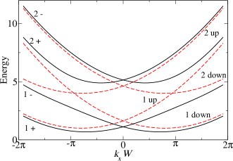
Figure 2: Energy levels of the two-band model (in units of $\hbar^{2}/2mW^{2}$) as a function of the dimensionless wave-vector $k_{x}W$ for the value $k_{\mathrm{SO}}W=\pi$ of the dimensionless spin-orbit parameter. The spectrum derived from the diagonalization of the two-band system, indicated in figure by $1+$, $1-$, $2+$, and $2-$ (solid lines), is compared with that from first-order perturbation theory, indicated by $1$ up, $1$ down, $2$ up, $2$ down (dashed lines).

As shown in Fig. 2, the eigenvalues (solid lines) do not show any intersection for $k_{x}$ different from zero. Therefore, the inter-band coupling removes the crossings of the first-order perturbation theory solution (dashed line). As a result, the energy eigenstates are no longer eigenstates of $\sigma_{z}$ [14] and the spin state depends on the wave-vector $k_{x}$. Close to the crossing point, the wave function of $1\uparrow$ and $2\downarrow$, for example, are strongly mixed in the mode $1+$. However, far from the intersection, the mode given by the diagonalization preserves the original behavior of the component wave-functions. For example, if we analyze the behavior of the eigenstate $\psi_{1+}(x,z)$, we get

$$\lim_{k_{x}\to-\infty}\psi_{1+}(x,z)=\psi_{1\uparrow}(x,z),\,\,\lim_{k_{x}\to\infty}\psi_{1+}(x,z)=\psi_{2\downarrow}(x,z).$$ (3ad)

The behavior of the two-band model shows a general trend: only taking into account the coupling between sub-bands the description is qualitatively correct. The crossing are artifacts of the lowest-order perturbation theory. The spectrum within the two-band model is reliable only for very narrow wires. In the general case, the low-energy description given by this model is too poor for the bands $2+$ and $2-$. This can be easily seen if one considers the energy values at $k_{x}=0$. In fact one gets for sub-bands $1\pm$ and $2\pm$, respectively, the achieved values are

$$\epsilon_{1\pm}=\frac{5\pi^{2}}{2}-\frac{1}{2}\sqrt{9\pi^{4}+\frac{1024{\bar{k}}_{\mathrm{SO}}^{2}}{9}}\,,$$ (3aea)

$$\epsilon_{2\pm}=\frac{5\pi^{2}}{2}+\frac{1}{2}\sqrt{9\pi^{4}+\frac{1024{\bar{k}}_{\mathrm{SO}}^{2}}{9}}.$$ (3aeb)

In the limit of small ${\bar{k}}_{\mathrm{SO}}$, they become

$$\epsilon_{1\pm}=\pi^{2}-\frac{256}{27\pi^{2}}{\bar{k}}_{\mathrm{SO}}^{2}\simeq\pi^{2}-0.961{\bar{k}}_{\mathrm{SO}}^{2}\,,$$ (3aeafa)

$$\epsilon_{2\pm}=4\pi^{2}+\frac{256}{27\pi^{2}}{\bar{k}}_{\mathrm{SO}}^{2}\simeq 4\pi^{2}+0.961{\bar{k}}_{\mathrm{SO}}^{2}.$$ (3aeafb)

From the comparison with the exact solution we find that the lowest sub-bands acquire a correction with the right sign and very close to the exact result, while the upper sub-bands have even the wrong sign. Therefore, in order to give a reasonable description of the low-energy part of the spectrum, more bands are necessary. This will also play an important role in the transport properties.

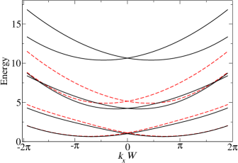
Figure 3: Energy levels of the wire (in units of $\hbar^{2}/2mW^{2}$) as a function of the dimensionless wave-vector $k_{x}W$ for the value $k_{\mathrm{SO}}W=\pi$ of the dimensionless spin-orbit parameter. The spectra derived from the diagonalization of the system with 3 sub-bands (solid line) and 2 sub-bands (dashed line) are shown.

3.3 Exact diagonalization

In order to verify the importance of including more than two sub-bands, one can directly diagonalize the Hamiltonian of the system [14]. This can be done considering the matrix elements (3r). In Fig. 3 we consider the diagonalization in the subspace of 3 spin degenerate bands. It is apparent that already at this level the corrections to the level energies and wave-functions are important for the second sub-band. For example, it is very close to the correct behavior at $k_{x}=0$. Considering $l$ sub-bands for the diagonalization, one is able to get a reliable behavior starting from sub-band 1 to $l-1$.

4 Ballistic Transport

In this section the issue is to study the quantum transport properties within the ballistic regime. The standard Landauer-Büttiker formalism will be employed. We will start considering a wire divided in two different regions: one with SOI and one without. Then we take the case of a quantum wire with a finite SOI region into account. The results are obtained within the approximation of the two-band model and those results will be compared with a numerical tight-binding method.

4.1 Single interface

We consider a QW divided in two main regions: in the right region ($x>0$) SOI is present while in the left region ($x<0$) it is not. The interface separating the two regions is considered to be sharp and is described by a $\delta$-like potential. The Hamiltonian of this hybrid system reads

$$\mathcal{H}_{\mathrm{hyb}} = {\vec{p}}\frac{1}{2m(x)}{\vec{p}}+V(z)+\frac{\hbar k_{\mathrm{SO}}(x)}{m_{\mathrm{SO}}}\left(\sigma_{z}p_{x}-\sigma_{x}p_{z}\right)$$ (3aeafag)

$$-i\sigma_{z}\frac{\hbar}{2m_{\mathrm{SO}}}\frac{\partial k_{\mathrm{SO}}(x)}{\partial x}+\frac{\hbar^{2}u}{2m(x)}\delta(x).$$

We assume that the mass and the strength of the SOI are piecewise constant with $k_{\mathrm{SO}}(x)=k_{\mathrm{SO}}\theta(x)$. For simplicity the mass is considered equal on both sides of the interface. The fourth term is necessary to get $\mathcal{H}_{\mathrm{hyb}}$ hermitian. At the interface the spinor eigenstates of $\mathcal{H}_{\mathrm{hyb}}$ have to be continuous, whereas their derivatives have a discontinuity $u-i\sigma_{z}k_{\mathrm{SO}}$ due to the SOI and to the $\delta$-like potential in $x=0$:

$$\psi(0^{+})=\psi(0^{-})\,,$$ (3aeafaha)

$$\left.\frac{\partial\psi(x)}{\partial x}\right|_{x=0^{+}}-\left.\frac{\partial\psi(x)}{\partial x}\right|_{x=0^{-}}=(u-\mathrm{i}\sigma_{z}k_{\mathrm{SO}})\psi(0).$$ (3aeafahb)

In order to study the effects of the sub-band hybridization on the transport properties, we start considering the injection of carriers only within the first sub-band. This can be achieved requiring that the second sub-band is behaving as an evanescent wave. In this context the Eqs. (3aeafaha-3aeafahb) are reduced to a set of two decoupled systems of four times four equations for the variables $r_{1+}$, $t_{1+}$, $r_{2-}$, $t_{2-}$ and $r_{1-}$, $t_{1-}$, $r_{2+}$, $t_{2+}$ respectively, where $t_{1(2),+(-)}$ and $r_{1(2),+(-)}$ are the transmission and the reflection amplitudes in the first (second) sub-band with spinor $+$ ($-$) respectively. The knowledge of the transmission and reflection amplitudes permits to evaluate the probability current and, as a consequence, the transmission probabilities for spin-up and spin-down carriers. Due to the presence of SOI only for $x>0$, the probability current has two different forms given by

$$\vec{j}=\displaystyle\frac{1}{m}\left\{\begin{array}[]{l r}\Re\left\{\psi^{\dagger}\vec{p}\,\psi\right\}&\mathrm{for}~{}x<0\\ \Re\left\{\psi^{\dagger}\left[\vec{p}+\hbar k_{\mathrm{SO}}\left(\hat{y}\times\vec{\sigma}\right)\right]\psi\right\}&\mathrm{for}~{}x>0\end{array}\right.$$ (3aeafahai)

where $\psi$ is the wave function solution of the system of Eqs. (3aeafaha-3aeafahb). A direct evaluation of the transmission probabilities [20] results in the following expressions:

$$T_{\uparrow}=\frac{|t_{1+}|^{2}}{k_{\mathrm{in}}}\left[k_{1+}(k_{\mathrm{in}})+k_{\mathrm{SO}}\langle\sigma_{z}\rangle_{1+}\right]\,,$$ (3aeafahaja)

$$T_{\downarrow}=\frac{|t_{1-}|^{2}}{k_{\mathrm{in}}}\left[k_{1-}(k_{\mathrm{in}})+k_{\mathrm{SO}}\langle\sigma_{z}\rangle_{1-}\right]\,,$$ (3aeafahajb)

where $k_{\mathrm{in}}$ is the injection momentum and $k_{1+}(k_{\mathrm{in}})$ and $k_{1-}(k_{\mathrm{in}})$ are the momentum relative to $k_{\mathrm{in}}$ for the two spin resolved sub-bands. The factors $\langle\sigma_{z}\rangle_{1+}$ and $\langle\sigma_{z}\rangle_{1-}$ are the expectation values of $\sigma_{z}$ on the two spin resolved sub-band wave functions and are defined as

$$\langle\sigma_{z}\rangle_{1\pm}=\pm\frac{1-f_{1}(\pm k_{1\pm})^{2}}{1+f_{1}(\pm k_{1\pm})^{2}}$$ (3aeafahajak)

where the function $f_{1}$ has been provided with Eq. (3ac). Because of the absence of SOI for $x<0$ the reflection probabilities are simply defined as $R_{\uparrow}=|r_{1+}|^{2}$ and $R_{\downarrow}=|r_{1-}|^{2}$. The system Hamiltonian $\mathcal{H}_{\mathrm{hyb}}$ is invariant under time-reversal symmetry and, as consequence, the following relations hold: $R_{\uparrow}=R_{\downarrow}$ and $T_{\uparrow}=T_{\downarrow}$. This means that spin-up and spin-down carriers are transmitted through the interface in the same way.

We consider the injection of a spin-unpolarized mixture of carriers with injection momentum $k_{\mathrm{in}}$. In terms of density matrix we have

$$\rho_{\mathrm{in}}=\frac{1}{2}|\uparrow\,\rangle\langle\,\uparrow|+\frac{1}{2}|\downarrow\,\rangle\langle\,\downarrow|$$ (3aeafahajal)

with the property that $\langle\sigma_{z}\rangle_{\mathrm{in}}=\mathrm{Tr}\{\rho_{\mathrm{in}}\sigma_{z}\}=0$. The density matrix of the transmitted carriers is expressed by the relation

$$\rho_{\mathrm{out}} = \frac{T_{\uparrow}}{T_{\uparrow}+T_{\downarrow}}|1+\rangle\langle 1+|+\frac{T_{\downarrow}}{T_{\uparrow}+T_{\downarrow}}|1-\rangle\langle 1-|$$ (3aeafahajam)

$$= \frac{1}{2}|1+\rangle\langle 1+|+\frac{1}{2}|1-\rangle\langle 1-|$$

where $|1\pm\rangle$ are the wave functions of the spin resolved sub-bands. We can now evaluate the polarization of the output carriers, this is expressed by

$$\langle\sigma_{z}\rangle_{\mathrm{out}} = \frac{1}{2}\langle\sigma_{z}\rangle_{1+}+\frac{1}{2}\langle\sigma_{z}\rangle_{1-}$$ (3aeafahajan)

$$= \frac{1}{2}\left(\frac{1-f_{1}(k_{1+})^{2}}{1+f_{1}(k_{1+})^{2}}-\frac{1-f_{1}(-k_{1-})^{2}}{1+f_{1}(-k_{1-})^{2}}\right).$$

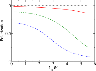
Figure 4: Polarization (3aeafahajan) as a function of the injection energy for $\bar{k}_{\mathrm{SO}}=0$ (dotted line), $\bar{k}_{\mathrm{SO}}=1$ (solid line), $\bar{k}_{\mathrm{SO}}=2$ (dashed line) and $\bar{k}_{\mathrm{SO}}=3$ (dotted-dashed line).

Figure (4) shows the polarization (3aeafahajan) as a function of the injection energy for various values of the SOI. The injection energy is limited within the first two spin-resolved sub-bands. It is clear that when SOI is zero (dotted line) there is no polarization, but as soon as the SOI is different from zero, the polarization gets a finite value, which increases as a function of SOI for a fixed energy. Those results are in accordance with Governale and Zülicke [14], who showed a negative polarization for carriers in the first two spin-resolved sub-bands and positive injection energies.

4.2 Wire with finite SOI region

We consider a QW composed of three parts: two external regions ($x<0$ and $x>L$) without SOI, and a central one ($0<x<L$) where SOI is present. We consider the hybrid system Hamiltonian of Eq. (3aeafag), with $k_{\mathrm{SO}}(x)=k_{\mathrm{SO}}\theta(x)\theta(L-x)$ and two $\delta$-like potentials of $x=0$ and $x=L$. Also in this case, for simplicity, the mass is assumed constant along the wire. As for the single interface case, the spinor eigenstates of $H_{\mathrm{hyb}}$ are continuous at the interfaces, whereas their derivatives have discontinuities in $x=0$ and $x=L$:

$$\psi(0^{+})=\psi(0^{-})\,,$$ (3aeafahajaoa)

$$\left.\frac{\partial\psi(x)}{\partial x}\right|_{x=0^{+}}-\left.\frac{\partial\psi(x)}{\partial x}\right|_{x=0^{-}}=(u-\mathrm{i}\sigma_{z}k_{\mathrm{SO}})\psi(0)\,,$$ (3aeafahajaob)

$$\psi(L^{+})=\psi(L^{-})\,,$$ (3aeafahajaoc)

$$\left.\frac{\partial\psi(x)}{\partial x}\right|_{x=L^{+}}-\left.\frac{\partial\psi(x)}{\partial x}\right|_{x=L^{-}}=(u+\mathrm{i}\sigma_{z}k_{\mathrm{SO}})\psi(L).$$ (3aeafahajaod)

As first step, we consider carriers with injection energy within the first two spin-resolved sub-bands and with evanescent waves for the following two. The Eqs. (3aeafahajaoa-3aeafahajaod) reduce to a set of two decoupled system of equations, with relevant terms $t_{\mathrm{R}1+}$, $t_{\mathrm{R}1-}$, $r_{\mathrm{L}1+}$ and $r_{\mathrm{L}1-}$. Those are practical for evaluating the transmission and the reflection probabilities for spin-up and spin-down carriers. As expected, because of the absence of SOI in the external regions we get

$$T_{\uparrow}=|t_{\mathrm{R}1+}|^{2}\,\,\,,\,\,\,T_{\downarrow}=|t_{\mathrm{R}1-}|^{2}\,,$$ (3aeafahajaoapa)

$$R_{\uparrow}=|r_{\mathrm{L}1+}|^{2}\,\,\,,\,\,\,R_{\downarrow}=|r_{\mathrm{L}1-}|^{2}.$$ (3aeafahajaoapb)

Due to time-reversal symmetry, it results that the value of the transmission probability $T_{\uparrow}$ for spin-up incoming carriers is equal to $T_{\downarrow}$ for incoming spin-down carriers. It is relevant to study transport properties when an unpolarized mixture of spin-up and spin-down carriers is injected into the system. The incoming and the outgoing density matrices are described by the expressions (3aeafahajal) and (3aeafahajam) respectively, where now the states $|1\pm\rangle$ are the output wave functions in the second region without SOI. As in the previous section we can evaluate the polarization as the average value of the $\sigma_{z}$ operator and obtain as result

$$\langle\sigma_{z}\rangle_{\mathrm{out}}=T_{\uparrow}-T_{\downarrow}=0.$$ (3aeafahajaoapaq)

The effect of spin polarization due to the first interface is completely cancelled by the second one, therefore it is not possible to observe any spin polarization [14]. This result can be also derived by a symmetry consideration: let us consider the scattering matrix $\mathcal{S}_{\mathrm{QW}}$ of the QW. In absence of a magnetic field time-reversal symmetry is preserved, therefore, as a consequence, for $\mathcal{S}_{\mathrm{QW}}$ holds the following important relation:

$$\mathcal{S}_{\mathrm{QW}}=\Sigma_{y}\mathcal{S}_{\mathrm{QW}}^{\dagger}\Sigma_{y}$$ (3aeafahajaoapar)

where $\Sigma_{y}=\left(\begin{array}[]{c c}\sigma_{y}&0_{2}\\ 0_{2}&\sigma_{y}\end{array}\right)$. It is clear for Eq. (3aeafahajaoapar) that in the case of only one conducting channel the spin-flip transmission terms must be zero and as consequence the polarization is absent [15].

As a further step, we study the transport properties when carriers are injected also within the second two spin-resolved sub-bands. In this limit all the evanescent modes are transformed in conducting ones. Using Eqs. (3aeafahajal) and (3aeafahajam) for the incoming and the out-coming density matrix, the polarization is expressed by

$$\langle\sigma_{z}\rangle_{\mathrm{out}} = \frac{1}{2}\left(\frac{T_{1+}(0)+T_{2+}(0)-T_{1-}(0)-T_{2-}(0)}{T_{1+}(0)+T_{2+}(0)+T_{1-}(0)+T_{2-}(0)}+\right.$$ (3aeafahajaoapas)

$$+\left.\frac{T_{1+}(\pi/2)+T_{2+}(\pi/2)-T_{1-}(\pi/2)-T_{2-}(\pi/2)}{T_{1+}(\pi/2)+T_{2+}(\pi/2)+T_{1-}(\pi/2)+T_{2-}(\pi/2)}\right),$$

where “$0$” and “$\pi/2$” denote incoming up- and down-carriers respectively.

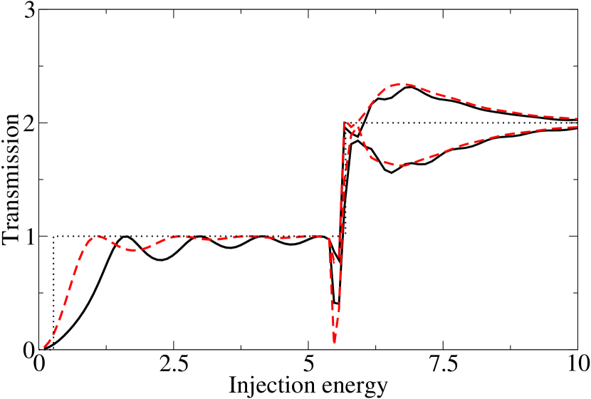
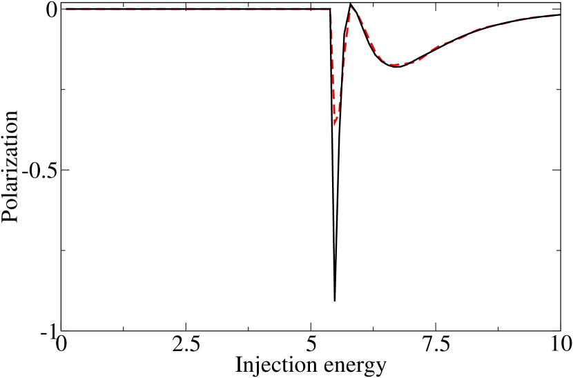
Figure 5: (Left Panel) Spin resolved transmissions as a function of the injection energy and for two different values of the transparency of the barriers: $u=1.0$ (solid lines) and $u=0.1$ (dashed lines). The dotted line indicates the opening of the sub-bands in absence of SOI. The dimensionless SOI is $\bar{k}_{\mathrm{SO}}=1.4$ and the central region is $L=3W$. (Right Panel) Spin polarization $\langle\sigma_{z}\rangle$ as a function of the injection energy and for two different value of the $\delta$-barrier transparency. The same parameters as in the left panel are used.

In Fig. 5 (left panel) we show the spin resolved transmissions as a function of the injection energy below and above the bottom of the second two sub-bands and for two values of the transparency $u$ of the interfaces (strength of the $\delta$-function potential in Eq. 3aeafag). The behavior below the threshold clearly shows Fabry-Perot oscillations due to multiple reflection effects within the central region, moreover the strength of those oscillations is decreasing for increasing transparency of the two $\delta$-barriers. A second important feature of the behavior is that up to the threshold, owing to the time-reversal symmetry, the two spin resolved components possess the same value. When the injection energy is crossing the bottom of the second two sub-bands, a new behavior appears. The two spin resolved transmissions take different values, the difference between those two is bigger near to the sub-band threshold and is decreasing with increasing energy. This can be well understood if we relate this phenomenon to the sub-band hybridization. As shown in Figs. 2 and 3 the SOI strongly modifies the parabolic-like behavior of the spin resolved sub-bands when new sub-bands are opening and this effect is vanishing at higher energies. In contrast to the results of Governale and Zülicke [14], Fig. 5 clearly shows how polarization effects can manifest themselves when also the second two spin-resolved sub-bands are involved into the transmission mechanism. This is more clear in Fig. 5 (right panel), where the polarization as a function of the injection energy is shown. The polarization is zero below the bottom of the second two sub-bands and has oscillating behavior above it. This particular shape of the polarization can be understood also in terms of formation of spin-dependent bound states at energies closer to the opening of the second two sub-bands. Those bound-state oscillations are clearly visible in the polarization pattern and it is evident how they are enhanced when the $\delta$-barrier transparency is decreased.

The effects on spin transport due to higher sub-bands can be numerically verified. For this purpose we employ a tight-binding model of the Hamiltonian (1), the spin-dependent scattering coefficients are obtained by projecting the corresponding spin-dependent Green function of the open system onto an appropriate set of asymptotic spinors defining incoming and outgoing channels. A real-space discretization of the Schrödinger equation in combination with a recursive algorithm for the computation of the corresponding Green function has been implemented [20]. This formalism allows a convenient treatment of different geometries as well as different sources of scattering within the same framework [21].

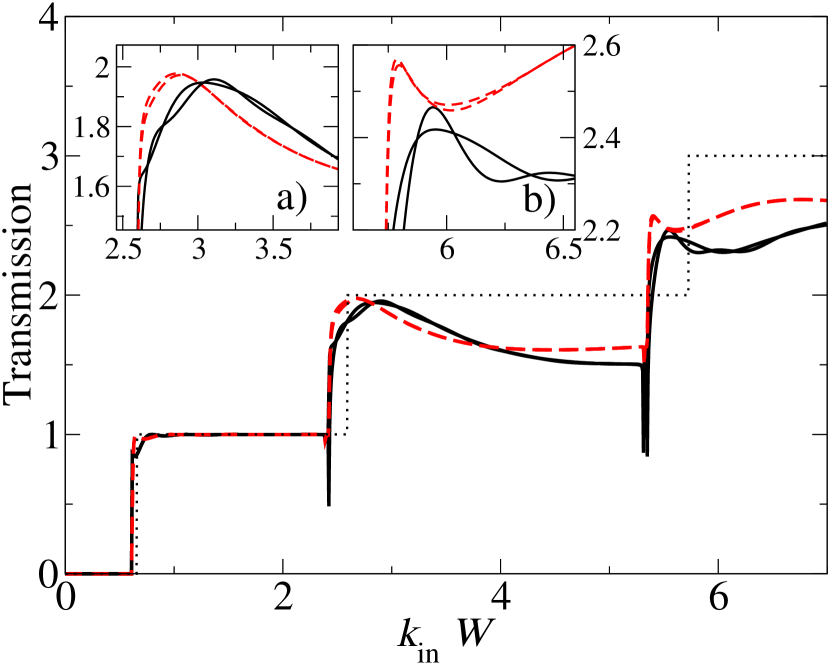
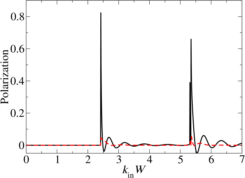
Figure 6: (Left Panel) Numerical spin resolved transmissions as a function of the injection energy and for two different values of the switching region of SOI: $L_{\mathrm{sr}}W^{-1}\sim 0.07$ (solid lines) and $L_{\mathrm{sr}}W^{-1}\sim 0.7$ (dashed lines). The dotted line indicates the opening of the sub-bands in absence of SOI. The dimensionless SOI is $\bar{k}_{\mathrm{SO}}=1.4$ and the central region is $L=3W+2L_{\mathrm{sr}}$. In the insets a) and b) are shown the magnification for the steps relative to the opening of the second and the third sub-band, respectively. (Right Panel) Spin polarization $\langle\sigma_{z}\rangle$ as a function of the injection of energy and for the two different values of $L_{\mathrm{sr}}W^{-1}$. The same parameters as in the left panel are used.

The $\delta$-barriers are introduced in the tight-binding calculation dividing the central region in three parts in order to modulate the switching region $L_{\mathrm{sr}}$ for the SOI. A long switching region will correspond to a high transparency, and vice versa. In Fig. 6 (left panel) we show the spin-resolved transmission as a function of the injection energy and for two different lengths of the switching region. The system parameters are chosen in order to have three active sub-bands in the case of injection within the highest energy allowed by the tight-binding approximation of the Hamiltonian (1). Injecting carriers within the first two spin-resolved sub-bands reproduces the result coming from time-reversal symmetry: spin-up and spin-down transmissions coincide. As soon as the second two sub-bands are opened we can observe a difference in their values. This difference tends to decrease for increasing energy but is, then, enhanced by the opening of the third two sub-bands [22]. This is clear from Fig. 6 (right panel), where we show the polarization as a function of the injection energy. Here it is also possible to observe how the strength of the polarization oscillations in strongly reduced changing the length of the switching region.

The polarizations at the opening of the second two spin-resolved sub-bands in the case of the two-band model (Fig. 5) and for the numerical tight-binding method (Fig. 6) show an opposite value. This can be well understood if we consider the polarization within the first and the second sub-band for an infinite long wire in the two-band and in the $N$-band models, respectively. In Fig. 7 we show the polarization for the first sub-band (upper Panel), it is evident that there is a small deviation of the two-band model (dashed lines) from the $N$-band model. But this deviation is stronger for the second sub-band (lower Panel) resulting in completely opposite value at large energies. This well reveals how the two-band model can only qualitatively reproduce the exact calculation, but is failing in the quantitative estimation.

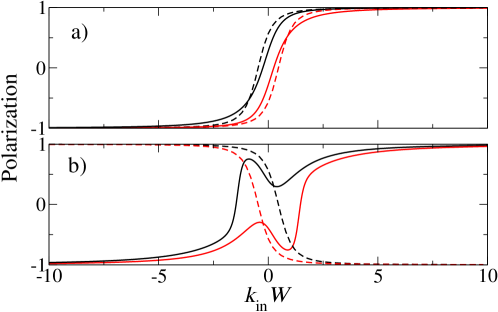
Figure 7: Polarization as a function of the injection energy for the two-band (dashed line) and the $N$-band (solid line) models, respectively. Panel a) first sub-band, Panel b) second sub-band. For both the Panels $N=50$.

5 Conclusions

We have studied the properties of a QW in the presence of Rashba SOI. The spectral properties have been investigated both from the point of view of the exact wave functions and within the second-order perturbation theory approach. Furthermore, a numerical diagonalization procedure has been implemented in order to study the spectral properties for the system in presence of $N$ sub-bands. We have used this last method with two sub-bands within the so called two-band model. We have shown that this is a good description for the full properties of the first sub-band but not of the second one. This model has also been used in order to study the transport properties of a system with an interface between a region with and without SOI. We have shown that the interface is spin selective and that the crossing of unpolarized carriers through the interface can give rise to a non-zero polarization. We have studied spin transport also injecting carriers within the first and the second sub-band. We have shown that at the opening of each new channel the sub-band hybridization can give rise to spin selective bound states reflecting in a oscillating spin polarization. Those results have been confirmed by numerical calculation obtained within the tight-binding approximation.

References

References

- [1] I. Žutíc, J. Fabian, and S. Das Sarma, Rev. Mod. Phys. 76, 323 (2004).
- [2] S.A. Wolf et al., Science 294, 1488 (2001).
- [3] S. Datta and B. Das, Appl. Phys. Lett. 56, 665 (1990).
- [4] G. Schmidt et al., Phys. Rev. B 62, 2790 (2000).
- [5] F.J. Jedema, A.T. Fillip, and B.J. van Wess, Nature 410, 345 (2001).
- [6] S.O. Valenzuela and M. Tinkham, Nature 442, 176 (2006).
- [7] G. Dresselhaus, Phys. Rev. 100, 580 (1955).
- [8] E. Rashba, Fiz. Tverd. Tela (Leningrad) 2, 1224 (1960), [Sov. Phys. Solid State 2, 1109 (1960)].
- [9] J. Nitta, T. Akazaki, H. Takayanagi, and T. Enoki, Phys. Rev. Lett. 78, 1335 (1997).
- [10] Th. Schäpers, J. Engels, T. Klocke, M. Hollfelder, and H. Lüth, J. Appl. Phys. 83, 4324 (1998).
- [11] D. Grundler, Phys. Rev. Lett. 84, 6074 (2000).
- [12] Th. Schäpers, J. Knobbe, and V. A. Guzenko, Phys. Rev. B 69, 235323 (2004)
- [13] F.Mireles and G.Kirczenow, Phys.Rev.B 64, 024426 (2001).
- [14] M. Governale, U. Zülicke, Phys. Rev. B 66, 073311 (2002).
- [15] Feng Zhai, and H. Q. Xu, Phys. Rev. Lett. 94, 246601 (2005).
- [16] V. M. Ramaglia, D. Bercioux, V. Cataudella, G.De Filippis, C.A. Perroni and F. Ventriglia, Eur. Phys. J. B 36, 365 (2003).
- [17] V.M. Ramaglia, D. Bercioux, V. Cataudella, G.De Filippis, and C.A. Perroni, J. Phys.: Condens Matter 16, 9143 (2004).
- [18] D. Bercioux, and V. M. Ramaglia, Superlattices Microstruct. 37, 337 (2005).
- [19] A. Laurincikas and Ramunas Garunkstis The Lerch Zeta-Function (Kluwer Academic Pub).
- [20] D. K. Ferry and S. M. Goodnick, Transport in Nanostructures (Cambridge University Press, 1997).
- [21] D. Frustaglia, M. Hentschel, and K. Richter, Phys. Rev. B 69, 155327 (2004).
- [22] Bound states owing to Fano resonances in quantum wire with Rashba spin-orbit interaction have been recently investigated also by Sánchez and Serra, Phys. Rev. B 74, 153313 (2006).