Evolution of a quantum spin system to its ground state: Role of entanglement and interaction symmetry

Abstract

We study the decoherence of two ferro- and antiferromagnetically coupled spins that interact with a frustrated spin-bath environment in its ground state. The conditions under which the two-spin system relaxes from the initial spin-up - spin-down state towards its ground state are determined. It is shown that the two-spin system relaxes to its ground state for narrow ranges of the model parameters only. It is demonstrated that the symmetry of the coupling between the two-spin system and the environment has an important effect on the relaxation process. In particular, we show that if this coupling conserves the magnetization, the two-spin system readily relaxes to its ground state whereas a non-conserving coupling prevents the two-spin system from coming close to its ground state.

I Introduction

The foundations of non-equilibrium statistical mechanics are still under debate (for a general introduction to the problem, see, e.g., Ref. balescu ; see also a very recent discussion popescu and Refs. therein). There is a common believe that a generic “central system” that interacts with a generic environment evolves into a state described by canonical ensemble (in the limit of low temperatures, this means the evolution to the ground state). Experience shows that this is true but a detailed understanding of this process, which is crucial for a rigorous justification of statistical physics and thermodynamics, are still lacking. In particular, in this context the meaning of “generic” is not clear. The key question is how the evolution to the equilibrium state depends on the details of the dynamics of the central system itself, on the environment, and on the interaction between the central system and environment.

In one of the first applications of computers to a basic physics problem Fermi, Pasta, and Ulam attempted to simulate the relaxation to thermal equilibrium of a system of interacting anharmonic oscillators ulam . The results obtained appeared to be counterintuitive, as we know now, due to complete integrability (in the continuum medium limit) of the model they simulated zaslavsky .

Bogoliubov bogoliubov has considered in a mathematically rigorous way the evolution to thermal equilibrium of a classical harmonic oscillator (central system) connected to the environment of classical harmonic oscillators which are already thermalized (for a generalization to a nonlinear Hamiltonian central system with one degree of freedom, see in Ref. KT, ). Also, for quantum systems this “bosonic bath” is the bath of choice, starting with the seminal works by Feynman and Vernon feynman and Caldeira and Leggett caldeira (for a review, see Ref. leggett, ). On the other hand, as we know now, the bosonic environment differs in many ways from, say, a spin-bath environment (such as nuclear spins) that dominate the decoherence processes of magnetic systems at low enough temperatures stamp . The evolution of quantum spin systems to the equilibrium state has been investigated in Refs. jens85, ; sait96, ; SKRO06, , for a very special class of spin Hamiltonians.

In terms of the modern “decoherence program” quantum systems interacting with an environment evolve to one of robust “pointer states”, the superposition of the pointer states being, in general, not a pointer state zeh ; zurek . The decoherence program is supposed to explain the “Schrödinger cat paradox”, that is, the inapplicability of the superposition principle to the macroworld. It is confirmed in many ways, indeed, that for the case where the interaction with environment is strong in comparison with typical energy differences for the central system classical “Schrödinger cat states” are the pointer states. At the same time, some less trivial pointer states have been found in computer simulations of quantum spin systems for some range of the model parameters ourPRL ; ourPLA ; ourPRE . In fact, the evolution of quantum spin systems to equilibrium is still an open issue (see also Refs. zurek2005, ; gedik, ; zurek2006, ). Recently, the effect of an environment of $N\gg 1$ spins on the entanglement of the two spins of the central system has attracted much attention ourPRL ; ourPLA ; ourPRE ; JETPLett ; Melikidze2004 ; Lucamarini2004 ; Wezel2005 ; Gao2005 ; YuanXZ2005 ; ZhangGF2005 ; Hamdouni2006 ; Slava2006 .

The relationship between the pointer states and the eigenstates of the Hamiltonian of central system is of special interest for the foundations of quantum statistical mechanics: The standard scenario assumes that the density matrix of the system at the equilibrium is diagonal in the basis of these eigenstates. Paz and Zurek paz have conjectured that pointer states are the eigenstates of the central system if the interaction of the central system with each degree of freedom of the environment is a perturbation, relative to the Hamiltonian of the central system. In view of the foregoing, it is important to establish the conditions under which this conjecture holds and to explore situations in which the interaction with environment can no longer be regarded as a perturbation with respect to the Hamiltonian of the central system.

In our Letter JETPLett , we reported a first collection of results for an antiferromagnetic Heisenberg system coupled to a variety of different environments. Our primary goal was to establish the conditions under which the central system relaxes from the initial spin-up - spin-down state towards its ground state, that is the maximally entangled singlet state. We found that environments that exhibit some form of frustration, such as spin glasses or frustrated antiferromagnets, may be very effective in producing a final state with a high degree of entanglement between the two central spins. We demonstrated that the efficiency of the decoherence process decreases drastically with the type of environment in the following order: Spin glass and random coupling of all spins to the central system; Frustrated antiferromagnet (triangular lattice with the nearest-neighbors interactions); Bipartite antiferromagnet (square lattice with the nearest-neighbors interactions); One-dimensional ring with the nearest-neighbors antiferromagnetic interactions JETPLett .

Competing interactions, frustration and glassiness provide a very efficient mechanism for decoherence whereas the difference between integrable and chaotic systems is less important ourPRE . Furthermore, we observed that for a fixed system size of the environment and in those cases for the decoherence is effective, different realizations of the random parameters do not significantly change the results. However, maximal entanglement in the central system was found for a relatively narrow range of the couplings between the environment spins and the interaction between the central spins and those of the environment.

Having established that the decoherence caused by a coupling to a frustrated, spin-glass-like environment can be a very effective, it is of interest to study in detail, the time evolution of the central system coupled to such an environment. In this paper, we consider as a central system, two ferro- or antiferromagnetically coupled spins that interact with a spin-glass environment. The interactions between each of the spin components of the latter are chosen randomly and uniformly from a specified interval centered around zero, making it very unlikely that there are conserved quantities in this three-component spin-glass. For the interaction of the central system with each of the spins of the environment we consider two cases.

In the first case, the couplings between the three components are generated using the same procedure as used for the environment. In the second case, the central system interacts with the environment via the $z$-components of the spins only. This implies that both the Hamiltonians that describe the central system (isotropic Heisenberg model) and the interaction between the central system the environment commutes with the total magnetization of the central system, hence the latter is conserved during the time evolution. In contrast to the naive picture in which the presence of conserved quantities reduces the decoherence, we find that the presence of a conserved quantity may affect significantly the nature of the stationary state to which the central system relaxes.

Table 1: The values of the correlation functions $\langle\mathbf{S}_{1}\cdot\mathbf{S}_{2}\rangle$, $\langle S_{1}^{z}S_{2}^{z}\rangle$, $\langle S_{1}^{x}S_{2}^{x}\rangle$, the total magnetization $M$, the concurrence $C$ and the magnetization $\langle S_{1}^{z}\rangle$ for different states of the central system.

$|\varphi\rangle$	$\langle\mathbf{S}_{1}\cdot\mathbf{S}_{2}\rangle$	$\langle S_{1}^{z}S_{2}^{z}\rangle$	$\langle S_{1}^{x}S_{2}^{x}\rangle$	$M$	$C$	$\langle S_{1}^{x}\rangle$
$\frac{1}{\sqrt{2}}\left(\left|\uparrow\downarrow\right\rangle-\left|\downarrow\uparrow\right\rangle\right)$	$-3/4$	$-1/4$	$-1/4$	$0$	$1$	$0$
$\frac{1}{\sqrt{2}}\left(\left|\uparrow\downarrow\right\rangle+\left|\downarrow\uparrow\right\rangle\right)$	$1/4$	$-1/4$	$1/4$	$0$	$1$	$0$
$\frac{1}{\sqrt{2}}\left(\left|\uparrow\uparrow\right\rangle-\left|\downarrow\downarrow\right\rangle\right)$	$1/4$	$1/4$	$-1/4$	$0$	$1$	$0$
$\frac{1}{\sqrt{2}}\left(\left|\uparrow\uparrow\right\rangle+\left|\downarrow\downarrow\right\rangle\right)$	$1/4$	$1/4$	$1/4$	$0$	$1$	$0$
$\left|\uparrow\downarrow\right\rangle$	$-1/4$	$-1/4$	$0$	$0$	$0$	$1/2$
$\left|\downarrow\uparrow\right\rangle$	$-1/4$	$-1/4$	$0$	$0$	$0$	$-1/2$
$\left|\uparrow\uparrow\right\rangle$	$1/4$	$1/4$	$0$	$1$	$0$	$1/2$
$\left|\downarrow\downarrow\right\rangle$	$1/4$	$1/4$	$0$	$-1$	$0$	$-1/2$

II Model

The model Hamiltonian that we study is defined by

$$H =H_{c}+H_{e}+H_{ce},$$

$$H_{c} =-J\mathbf{S}_{1}\cdot\mathbf{S}_{2},$$

$$H_{e} =-\sum_{i=1}^{N-1}\sum_{j=i+1}^{N}\sum_{\alpha}\Omega_{i,j}^{(\alpha)}I_{i}^{\alpha}I_{j}^{\alpha},$$

$$H_{ce} =-\sum_{i=1}^{2}\sum_{j=1}^{N}\sum_{\alpha}\Delta_{i,j}^{(\alpha)}S_{i}^{\alpha}I_{j}^{\alpha},$$ (1)

where the exchange integrals $J$ and $\Omega_{i,j}^{(\alpha)}$ determine the strength of the interaction between spins $\mathbf{S}_{n}=\left(S_{n}^{x},S_{n}^{y},S_{n}^{z}\right)$ in the central system ($H_{c}$), and the spins $\mathbf{I}_{n}=\left(I_{n}^{x},I_{n}^{y},I_{n}^{z}\right)$ in the environment ($H_{e}$), respectively. The exchange integrals $\Delta_{i,j}^{(\alpha)}$ control the interaction ($H_{ce}$) of the central system with its environment. In Eq. (1), the sum over $\alpha$ runs over the $x$, $y$ and $z$ components of spin-$1/2$ operators $\mathbf{S}$ and $\mathbf{I}$. The exchange integral $J$ of the central system can be positive or negative, the corresponding ground state of the central system being ferromagnetic or antiferromagnetic, respectively.

In the sequel, we will use the term “Heisenberg-like” $H_{ce}$ ($H_{e}$) to indicate that $\Delta_{i,j}^{(\alpha)}$ ($\Omega_{i,j}^{(\alpha)}$) are uniform random numbers in the range $[-\Delta|J|,\Delta|J|]$ ($[-\Omega|J|,\Omega|J|]$) for all $\alpha$’s and use the expression “Ising-like” $H_{ce}$ ($H_{e}$) to indicate that $\Delta_{i,j}^{(x,y)}=0$ ($\Omega_{i,j}^{(x,y)}=0$), and that $\Delta_{i,j}^{(z)}$ ($\Omega_{i,j}^{(z)}$) are dichotomic random variables taking the values $\pm\Delta$ ($\pm\Omega$). The parameters $\Delta$ and $\Omega$ determine the maximum strength of the interactions.

The quantum state of central system is completely determined by its reduced density matrix, the $4\times 4$ matrix that is obtained by computing the trace of the full density matrix over all but the four states of the central system. In our simulation work, the whole system is assumed to be in a pure state, denoted by $|\Psi(t)\rangle$. Although the reduced density matrix contains all the information about the central system, it is often convenient to characterize the state of the central system by other quantities such as the correlation functions $\langle\Psi(t)|\mathbf{S}_{1}\cdot\mathbf{S}_{2}|\Psi(t)\rangle$, $\langle\Psi(t)|S_{1}^{z}S_{2}^{z}|\Psi(t)\rangle$, and $\langle\Psi(t)|S_{1}^{x}S_{2}^{x}|\Psi(t)\rangle$, the single-spin magnetizations $\langle\Psi(t)|S_{1}^{x}|\Psi(t)\rangle$, $\langle\Psi(t)|S_{2}^{x}|\Psi(t)\rangle$, and $M\equiv\langle\Psi(t)|\left(S_{1}^{z}+S_{2}^{z}\right)|\Psi(t)\rangle$, and the concurrence $C(t)$ Wootters97 ; Wootters98 . The concurrence, which is a convenient measure for the entanglement of the spins in the central system, is equal to one if the state of central system is unchanged under a flip of the two spins, and is zero for an unentangled pure state such as the spin-up - spin-down state. In Table 1, we show the values of these quantities for to different states of the central system.

As the energy of central system is given by $-J\langle\Psi(t)|\mathbf{S}_{1}\cdot\mathbf{S}_{2}|\Psi(t)\rangle$, it follows from Table 1 that the four eigenstates of the central system $H_{c}$ are given by

$$\left|S\right\rangle = \frac{\left|\uparrow\downarrow\right\rangle-\left|\downarrow\uparrow\right\rangle}{\sqrt{2}},$$

$$\left|T_{0}\right\rangle = \frac{\left|\uparrow\downarrow\right\rangle+\left|\downarrow\uparrow\right\rangle}{\sqrt{2}},$$

$$\left|T_{1}\right\rangle = \left|\uparrow\uparrow\right\rangle,$$

$$\left|T_{-1}\right\rangle = \left|\downarrow\downarrow\right\rangle,$$ (2)

satisfying

$$H_{c}\left|S\right\rangle=E_{S}\left|S\right\rangle,\text{ }H_{c}\left|T_{1,0,-1}\right\rangle=E_{T}\left|T_{1,0,-1}\right\rangle,$$ (3)

where $E_{S}=3J/4$ and $E_{T}=-J/4$.

¿From Table 1, it is clear that the singlet state $\left|S\right\rangle$ is most easily distinguished from the others as the central system is in the singlet state if and only if $\langle\mathbf{S}_{1}\cdot\mathbf{S}_{2}\rangle=-3/4$. To identify other states, we usually need to know at least two of the quantities listed in Table 1. For example, to make sure that the system is the triplet state $\left|T_{0}\right\rangle$, the values of $\langle\mathbf{S}_{1}\cdot\mathbf{S}_{2}\rangle$ and $\langle S_{1}^{z}S_{2}^{z}\rangle$ should match with the corresponding entries of Table 1. Likewise, the central system will be in the state $\left|\uparrow\uparrow\right\rangle$ if $\langle\mathbf{S}_{1}\cdot\mathbf{S}_{2}\rangle$ and $M$ agree with the corresponding entries of Table 1.

In general, we monitor the effects of the decoherence by plotting the time dependence of the two-spin correlation function $\langle\mathbf{S}_{1}\cdot\mathbf{S}_{2}\rangle$ and the matrix elements of the density matrix. We compute the matrix elements of the density matrix in the basis of eigenvectors of the central system (see Eq. (II)). If necessary to determine the nature of the state, we consider all the quantities listed in Table 1.

The simulation procedure is as follows. First, we select a set of model parameters. Next, we compute the ground state $\left|\phi_{0}\right\rangle$ of the environment and, for reference, the ground state of the whole system also. The spin-up – spin-down state ($\left|\uparrow\downarrow\right\rangle$) is taken as the initial state of the central system. Thus, the initial state of the system reads $\left|\Psi(t=0)\right\rangle\rangle=\left|\uparrow\downarrow\right\rangle\left|\phi_{0}\right\rangle$ and is a product state of the state of the central system and the ground state of the environment which, in general is a (very complicated) linear combination of the $2^{N}$ basis states of the environment.

The time evolution of the whole system is obtained by solving the time-dependent Schrödinger equation for the many-body wave function $|\Psi(t)\rangle$, describing the central system plus the environment. The numerical method that we use is described in Ref. method . It conserves the energy of the whole system to machine precision.

In our model, decoherence is solely due to fact that the initial product state $|\Psi(0)\rangle=|\uparrow\downarrow\rangle$ evolves into an entangled state of the whole system. The interaction with the environment causes the initial pure state of the central system to evolve into a mixed state, described by a reduced density matrix neumann , obtained by tracing out all the degrees of freedom of the environment feynman ; leggett ; zeh ; zurek . If the Hamiltonian of the central system $H_{c}$ is a perturbation, relative to the interaction Hamiltonian $H_{ce}$, the pointer states are eigenstates of $H_{ce}$ zurek ; paz . On the other hand, if $H_{ce}$ is much smaller than the typical energy differences in the central system, the pointer states are eigenstates of $H_{c}$, that is, they may be singlet or triplet states. In fact, as we will show, the selection of the eigenstate as the pointer state is also determined by the state and the dynamics of the environment.

In the simulations that we discuss in the paper, the interactions between the central system and the environment are either Ising or Heisenberg-like. The interesting regime for decoherence occurs when each coupling of the central system with the environment is weak, that is, $\Delta\ll|J|$, but there is of course nothing that prevents us from performing simulations outside this regime. The interaction within the environment are taken to be Heisenberg-like, $\Omega$ being a parameter that we change.

III Heisenberg-like $H_{ce}$

III.1 Ferromagnetic central system

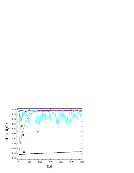
Figure 1: (Color online) The time evolution of the correlation $\langle\Psi(t)|\mathbf{S}_{1}\cdot\mathbf{S}_{2}|\Psi(t)\rangle$ of the ferromagnetic central system with Heisenberg-like $H_{ce}$ and $H_{e}$. The model parameters are $\Delta=0.15$ and a: $\Omega=0.075$; b: $\Omega=0.15$; c: $\Omega=0.20$; d: $\Omega=0.30$; e: $\Omega=1$. The number of spins in the environment is $N=14$.

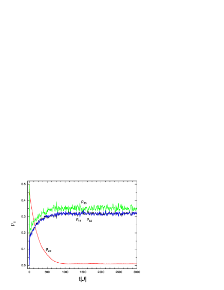
Figure 2: (Color online) The time evolution of the diagonal matrix elements of the reduced density matrix of the central system for $\Delta=0.15$ and $\Omega=0.15$ (case (b) of Fig. 1). The number of spins in the environment is $N=14$.

In this section, we consider a ferromagnetic ($J=1$) central system that interacts with the environment via a Heisenberg-like interaction (recall that throughout this paper the environment itself is always Heisenberg-like).

In Fig. 1, we present simulation results for the two-spin correlation function for different values of the parameter $\Omega$ that determines the maximum strength of the coupling between the $N(N-1)/2$ pairs of spins in the environment. Clearly, in case (a), the relaxation is rather slow and confirming that there is relaxation to the ground state requires a prohibitively long simulation. For cases (b) – (d), the results are in concert with the intuitive picture of relaxation due to decoherence: The correlation shows the relaxation from the up-down initial state of the central system to the fully polarized state in which the two spins point in the same direction.

An important observation is that our data convincingly shows that it is not necessary to have a macroscopically large environment for decoherence to cause relaxation to the ground state: A spin-glass with $N=14$ spins seems to be more than enough to mimic such an environment. This observation is essential for numerical simulations of relatively small systems to yield the correct qualitative behavior.

Qualitative arguments for the high efficiency of the spin-glass bath were given in Ref. JETPLett, . Since the spin-glasses possess a huge amount of the states that have an energy close to the ground state energy but have wave functions that are very different from the ground state, the orthogonality catastrophe, blocking the quantum interference in the central system zeh ; zurek is very strongly pronounced in this case.

This conclusion is further supported by Fig. 2 where we show the diagonal elements of the reduced density matrix for case (b). After reaching the steady state, the nondiagonal elements exhibit minute fluctuations about zero and are therefore not shown. From Fig. 2, it is then clear that central system relaxes to a mixture of the (spin-up, spin-up), (spin-down, spin-down), and triplet state, as expected of intuitive grounds. In case (e), the characteristic strength of the interactions between the spins in the environment is of the same order as the exchange coupling in the central system ($\Omega\approx J$), a regime in which there clearly is significant transfer of energy, back-and-forth, between the central system and the environment.

¿From the data for (b) – (d), shown in Fig. 1, we conclude that the time required to let the central system relax to a state that is close to the ground state depends on the energy scale ($\Omega$) of the random interactions between the spins in the environment. As it is difficult to define the point in time at which central system has reached its stationary state, we have not made an attempt to characterize the dependence of a relaxation time on $\Omega$.

III.2 Antiferromagnetic central system

We now consider what happens if we replace the ferromagnetic central system by an antiferromagnetic one.

The main difference between the antiferromagnetic and the ferromagnetic central system is that the ground state of the former is maximally entangled (a singlet) whereas the latter is a fully polarized product state.

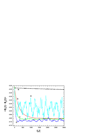
Figure 3: (Color online) The time evolution of the correlation $\langle\Psi(t)|\mathbf{S}_{1}\cdot\mathbf{S}_{2}|\Psi(t)\rangle$ of the antiferromagnetic central system with Heisenberg-like $H_{ce}$ and $H_{e}$. The model parameters are $\Delta=0.15$ and a: $\Omega=0.075$; b: $\Omega=0.15$; c: $\Omega=0.20$; d: $\Omega=0.30$; e: $\Omega=1$. The number of spins in the environment is $N=14$.

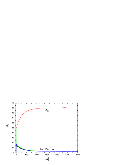
Figure 4: (Color online) The time evolution of the diagonal matrix elements of the reduced density matrix of the central system for $\Delta=0.15$ and $\Omega=0.15$ (case (b) of Fig. 3). The number of spins in the environment is $N=14$.

In Fig. 3, we present simulation results for the two-spin correlation function for different values of the parameter $\Omega$. In passing, we mention that in our simulations, we change the sign of $J$ only, that is we use the same parameters for $H_{ce}$ and $H_{e}$ as in the corresponding simulations of the ferromagnetic case. Apart from the change is sign, the curves for all cases (a–e) in Fig. 1 and Fig. 3 are qualitatively similar. However, this is a little deceptive.

As for the ferromagnetic central system, in case (a), the relaxation is rather slow and confirming that there is relaxation to the ground state requires a prohibitively long simulation. In case (e), we have $\Omega\approx|J|$ and as already explained earlier, this case is not of immediate relevance to the question addressed in this paper. For cases (b) – (d), the results are in concert with the intuitive picture of relaxation due to decoherence except that the central system does not seem to relax to its true ground state. Indeed, the two-spin correlation relaxes to a value of about $0.65$ – $0.70$, which is much further away from the ground state value $-3/4$ than we would have expected on the basis of the results of the ferromagnetic central system. In the true ground state of the whole system, the value of the two-spin correlation in case (b) is $-0.7232$, hence significantly lower than than the typical values, reached after relaxation. On the one hand, it is clear (and to be expected) that the coupling to the environment changes the ground state of the central system, but on the other hand, our numerical calculations show that this change is too little to explain the apparent difference with the results obtained from the time-dependent solution.

In Fig. 4, we plot the diagonal matrix elements of the density matrix (calculated in the basis for which the Hamiltonian of the central system is diagonal) for case (b). From this data and the fact that the nondiagonal elements are negligibly small (data not shown), we conclude that the central system relaxes to a mixture of the singlet state and the (spin-up, spin-up) and (spin-down, spin-down) states, the former having much more weight ($0.9$ to $0.05$) than the two latter states. Thus, at this point, we conclude that our results suggest that decoherence is less effective for letting a central system relax to its ground state if this ground state is entangled than if it is a product state. Remarkably, this conclusion changes drastically when we replace the Heisenberg-like $H_{ce}$ by an Ising-like $H_{ce}$, as we demonstrate next.

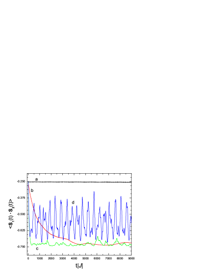
Figure 5: (Color online) The time evolution of the correlation $\langle\Psi(t)|\mathbf{S}_{1}\cdot\mathbf{S}_{2}|\Psi(t)\rangle$ of the antiferromagnetic central system with Ising-like $H_{ce}$ and Heisenberg-like $H_{e}$. The model parameters are $\Delta=0.075$ and a: $\Omega=0.075$; b: $\Omega=0.15$; c: $\Omega=0.30$; d: $\Omega=1$. The number of spins in the environment is $N=16$.

IV Ising-like $H_{ce}$

In our simulation, the initial state of the central system is $\left|\uparrow\downarrow\right\rangle$ and this state has total magnetization $M=0$. For Ising $H_{ce}$ with Heisenberg-like $H_{e}$ coupling, the magnetization $M$ of the central system commutes with the Hamiltonian (1) of the whole system. Therefore, the magnetization of the central system is conserved during the time evolution, and the central system will always stay in the subspace with $M=0$. In this subspace, the ground state for antiferromagnetic central system is the singlet state $|S\rangle$ while for the ferromagnetic central system the ground state (in the $M=0$ subspace) is the entangled state $|T_{0}\rangle$. Thus, in the Ising-like $H_{ce}$, starting from the initial state $\left|\uparrow\downarrow\right\rangle$, the central system should relax to an entangled state, for both a ferro- or antiferromagnetic central system.

If the initial state of the central system is $\left|\uparrow\downarrow\right\rangle$, it can be proven (see Appendix) that

$$\langle\Psi(t)|\mathbf{S}_{1}\cdot\mathbf{S}_{2}|\Psi(t)\rangle_{F}+\langle\Psi(t)|\mathbf{S}_{1}\cdot\mathbf{S}_{2}|\Psi(t)\rangle_{A}=-\frac{1}{2},$$ (4)

where the subscript $F$ and $A$ refer to the ferro- antiferromagnetic central system, respectively. Likewise, for the concurrence we find $C_{F}\left(t\right)=C_{A}\left(t\right)$ and similar symmetry relations hold for the other quantities of interest. Of course, this symmetry is reflected in our numerical data also, hence we can limit ourselves to presenting data for the antiferromagnetic central system with Ising-like $H_{ce}$ and Heisenberg-like $H_{e}$.

In Fig. 5, we present simulation results for the two-spin correlation function for different values of the parameter $\Omega$. Notice that compared to Figs. 1– 4, we show data for a time interval that is three times larger. For the cases (b,c), the main difference between Fig. 3 and Fig. 5 is that for the latter and unlike for the former, the central system relaxes to a state that is very close to the ground state. Thus, we conclude that the presence of a conserved quantity (the magnetization of the central system) acts as a catalyzer for relaxing to the ground state. Although it is quite obvious that by restricting the time evolution of the system to the $M=0$ subspace, we can somehow force the system to relax to the entangled state, it is by no means obvious why the central system actually does relax to a state that is very close to the ground state.

Intuitively, we would expect that the presence of a conserved quantity hinders the relaxation and indeed, that is what we observe in cases (a,b) where the relaxation is much slower than in cases (a,b) of Fig. 1 or of Fig. 3. Notwithstanding this, in the presence of a conserved quantity, the central system relaxes to a state that is much closer to true ground state than it would relax to in the absence of this conserved quantity.

V Role of $\Delta$

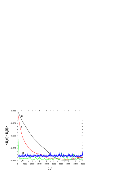
Figure 6: (Color online) The time evolution of the correlation $\langle\Psi(t)|\mathbf{S}_{1}\cdot\mathbf{S}_{2}|\Psi(t)\rangle$ of the antiferromagnetic central system with Ising-like $H_{ce}$ and Heisenberg-like $H_{e}$. a: $\Delta=0.0375$ and $\Omega=0.15$; b: $\Delta=0.075$ and $\Omega=0.15$; c: $\Delta=0.075$ and $\Omega=0.3$; d: $\Delta=0.15$ and $\Omega=0.3$. The number of spins in the environment is $N=16$.

Now, we study the effect of changing the strength $\Delta$ of the coupling between central system and the environment. For a qualitative discussion of this aspect, it suffices to consider the case of Ising-like $H_{ce}$, as we have seen that then, the central system most easily relaxes to its ground state.

In Fig. 6, we present some representative simulation results for the two-spin correlation function for different values of the parameters $\Delta$ and $\Omega$. By simply comparing the time intervals of the plots for cases (a,b) and (c,d), it is immediately clear that the speed of relaxation changes drastically with $\Delta$. For a “slow” environment (small enough $\Omega$) the effect is rather trivial, namely, the larger $\Delta$ the faster the relaxation. In the case (c) the system comes close to the triplet state in comparison with (d), probably, since the perturbation of the ground state of the central system is smaller.

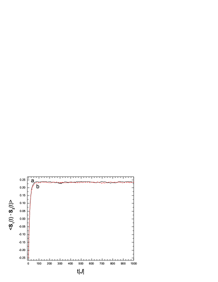
Figure 7: (Color online) The time evolution of the correlation $\langle\Psi(t)|\mathbf{S}_{1}\cdot\mathbf{S}_{2}|\Psi(t)\rangle$ of a ferromagnetic central system with Heisenberg-like $H_{ce}$ and Heisenberg-like $H_{e}$ with $\Delta=0.15$ and $\Omega=0.3$. Initial state of the environment is solid line (a): ground state; dashed line (b): close to but not the same as the ground state. The number of spins in the environment is $N=14$.

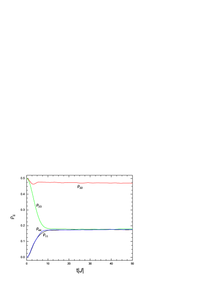
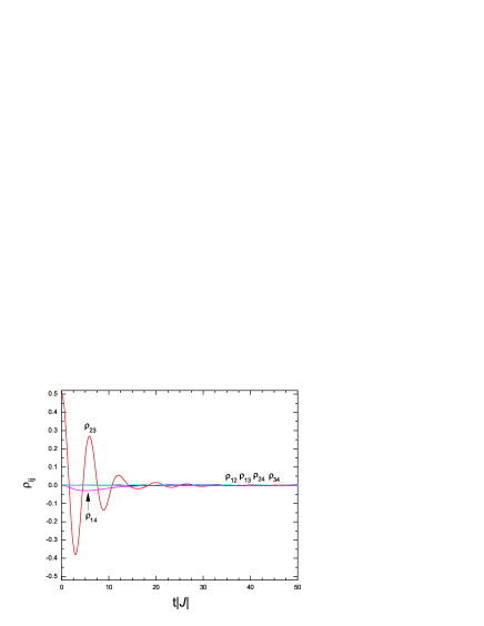
Figure 8: (Color online) The time evolution of the diagonal elements (left panel) and the real parts of the off-digonal elements (right panel) of the reduced density matrix in the antiferromagnetic central system, with Heisenberg-like $H_{ce}$ and Heisenberg-like $H_{e}$ ($\Delta=0.15$ and $\Omega=0.15$). The initial state of the central two spins is the up-down state, and the environment is initially in a random state. The number of spins in the environment is $N=14$.

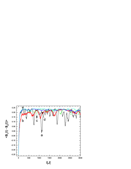
Figure 9: (Color online) The time evolution of the correlation $\langle\Psi(t)|\mathbf{S}_{1}\cdot\mathbf{S}_{2}|\Psi(t)\rangle$ of a ferromagnetic central system with Heisenberg-like $H_{ce}$ and Heisenberg-like $H_{e}$ with $\Delta=0.15$ and $\Omega=0.3$. The number of spins in the environment is a: $N=8$; b: $N=9$; c: $N=10$; d: $N=11$; e: $N=12$.

VI Sensitivity of the results to characteristics of the environment

Finally, we study the effect of small changes to the initial state of the environment and of the number of spins in the environment.

For the spin glasses, the true ground state is rather hardly reachable and there are a lot of states with a very close energy but essentially different characteristics. To check how relevant it can be for our observations, we replace the environment ground state by one of such states and study the time evolution of the central system as we did before. In Fig. 7, we show typical results for a ferromagnetic central system with Heisenberg-like $H_{ce}$ and Heisenberg-like $H_{e}$. In the initial state, the energy of the environment $E_{b}=-2.247$, which is a little bit higher than the ground-state energy of the environment $E_{a}=-2.321$. The time evolution of the correlation function of the two central spins for the cases (a) and (b) (see Fig. 7) clearly demonstrates that in both cases, the central system evolves to the ground state, and that the dynamics of this evolution is also very similar. This confirms that as long as the energy of the initial state of the environment is close to its ground state energy, the qualitative features of the decoherence process remain the same. If, on the other hand, we prepare the environment in a random state (which, roughly speaking, corresponds to a very high temperature), the central system does not relax to its ground state but to a mixed state with a diagonal density matrix, as expected (see Fig. 8).

Second, we study the effect of finite size of the environment on the decoherence process. Some typical results for a ferromagnetic central system with Heisenberg-like $H_{ce}$ and Heisenberg-like $H_{e}$ with different numbers of the environment spins $N$ are shown in Fig. 9. It looks reasonable to define the border between a mesoscopic and a macroscopic environment as a value of $N$ for which the oscillations in the two-particle correlation are no longer well-defined. Thus, on the basis of the data displayed in Fig. 9 one can say that $N\approx 11$ is large enough for the spin-glass environment to mimic the macroscopic system. Needless to say, this statement is very qualitative but, in any case, the $N$ dependence of the results shown in Fig. 9 demonstrate the effectiveness of the spinglass as a model environment to study decoherence processes with rather modest requirements to the environment size.

VII Summary

We have presented the results of simulations that address the question how a small quantum system evolves to its ground state when it is brought in contact to an environment consisting of quantum spins. Our systematic study confirms the suggestion of Ref. JETPLett, that the use of spin-glass thermal bath is indeed a very efficient way to simulate decoherence processes. Environments containing $14$ – $16$ spins are sufficiently large to induce a complete decay of the Rabi oscillations, this in sharp contrast to environments that have a more simple structure, such as spin-chains or square lattices JETPLett .

In general, it turns out that the relaxation to the ground state is a more complicated process that one would naively expect, depending essentially on the ratio between parameters of the interaction and environment Hamiltonians. Two general conclusions are: (i) the central system more easily evolves to its ground state when the latter is less entangled (e.g., up-down state compared to the singlet) and (ii) constraints on the system such as existence of additional integrals of motion can make the evolution to the ground state more efficient.

At the first sight, the latter statement looks a bit counterintuitive since it means that it may happen that a more regular system exhibits stronger relaxation than a chaotic one. The reason that is may happen is that the larger the dimensionality of available Hilbert space for the central system is, the more complicated the decoherence process is due to appearance of the whole hierarchy of the decoherence times for different elements of the reduced density matrix. A manifestation of this phenomenon has been observed earlier ourPRL : Under certain conditions, the same central system as studied here (four by four reduced density matrix) displays “quantum oscillations without quantum coherence” whereas for a single spin in magnetic field (two by two reduced density matrix) decoherence can, relatively easily, suppress the Rabi oscillations completely.

We believe that these results can stimulate further development and clarification of the “decoherence program” zurek ; ZURE98 . Assuming that the interaction with an environment is weak enough, a hypothesis that the pointer states should be the eigenstates of the Hamiltonian of the central system was proposed paz , with the very ambitious aim to explain the basic phenomenon of “quantum jumps”. In this paper, we demonstrate that, apart from just a strength of different interactions, also their symmetry and the amount of entanglement of the ground state of the central system may play an essential role. Among the cases which we consider in this paper, there are two situations where the standard decoherence scenario works as envisaged paz . If the ground state is not entangled (as in the case of the up-down state for the case of ferromagnetic interactions) or if the Hilbert space is restricted due to some conservation laws (as for the singlet ground state in the Ising-type interaction Hamiltonian), the central system clearly evolves to its ground state, supposed to be the pointer state according to Ref. paz . However, if the ground state of the central system is the fully entangled singlet state, and interaction Hamiltonian is generic, without symmetries, the system evolves to some mixture of the ground state and excited states. Of course, the data presented here are not sufficient to make strong, general statements about the character of the pointer states but we hope that, at least, our work will stimulate further research to establish the conditions under which the conjecture that the pointer states are the eigenstates of the central system hold.

Appendix

For the Hamiltonian Eq. (1), if $\Delta_{i,j}^{(x)}=\Delta_{i,j}^{(y)}=0$, $H_{ce}$ is Ising-like and it is easy to prove that $[M,H]=0$, implying that the magnetization of the central two spins is a conserved quantity. In our simulations, we take as the initial state of the central system the spin-up - spin-down state ($|\uparrow\downarrow\rangle=(|S\rangle+|T_{0}\rangle)/\sqrt{2}$). Hence, because $[M,H]=0$, the central spin system will always stay in the subspace of $M=0$. Thus, at any time $t$, the state of the whole system can be written as

$$|\Psi(t)\rangle=|S\rangle|\phi_{S}(t)\rangle+|T_{0}\rangle|\phi_{T_{0}}(t)\rangle,$$ (5)

where $|\phi_{S}\rangle$ and $|\phi_{T_{0}}\rangle$ denote the states of the environment.

Let us denote by $\{|\psi_{i}\rangle\}$ a complete set of states of the environment. Within the subspace spanned by the states $\{|S\rangle|\psi_{i}\rangle,|T_{0}\rangle|\psi_{i}\rangle\}$, the Hamiltonian Eq. (1) can be written as

$$H = E_{S}|S\rangle\langle S|+E_{T}|T_{0}\rangle\langle T_{0}|+H_{e}$$ (6)

$$-\frac{1}{2}\sum_{j=1}^{N}(\Delta_{1,j}^{(z)}-\Delta_{2,j}^{(z)})\left(|S\rangle\langle T_{0}|+|T_{0}\rangle\langle S|\right)I_{j}^{z},$$

where we used $\langle S|S_{1}^{z}|S\rangle=\langle T_{0}|S_{1}^{z}|T_{0}\rangle=\langle S|S_{2}^{z}|S\rangle=\langle T_{0}|S_{2}^{z}|T_{0}\rangle=0$, $\langle T_{0}|S_{1}^{z}|S\rangle=1/2$, and $\langle T_{0}|S_{2}^{z}|S\rangle=-1/2$.

Introducing a pseudo-spin $\sigma=(\sigma^{x},\sigma^{y},\sigma^{z})$ such that the eigenvalues $+1$ and $-1$ of $\sigma^{z}$ correspond to the states $|S\rangle$ and $|T_{0}\rangle$, respectively, Eq. (6) can be written as

$$H = \frac{E_{S}-E_{T}}{2}+\frac{E_{S}+E_{T}}{2}\sigma^{z}+H_{e}$$ (7)

$$-\frac{1}{2}\sum_{j=1}^{N}(\Delta_{1,j}^{(z)}-\Delta_{2,j}^{(z)})I_{j}^{z}\sigma^{x},$$

showing that in the case of Ising-like $H_{ce}$, the model Eq. (1) with two central spins is equivalent to the model Eq. (7) with one central spin.

¿From Eq. (7), it follows immediately that the Hamiltonian is invariant under the transformation $\{J,\sigma^{z}\}\rightarrow\{-J,-\sigma^{z}\}$. Indeed, the first, constant term in Eq. (7) is irrelevant and we can change the sign of the second term by rotating the speudo-spin by 180 degrees about the $x$-axis. Therefore, if the initial state is invariant under this transformation also, the time-dependent physical properties will not depend on the choice of the sign of $J$, hence the ferro- and antiferromagnetic system will behave in exactly the same manner.

For the case at hand, the initial state can be written as $(|S\rangle+|T_{0}\rangle)|\phi_{0}\rangle/\sqrt{2}$, which is trivially invariant under the transformation $\sigma^{z}\rightarrow-\sigma^{z}$. Summarizing: For Ising-like $H_{ce}$ ($\Delta_{i,j}^{(x)}=\Delta_{i,j}^{(y)}=0$), and an initial state that is invariant for the transformation $|S\rangle\leftrightarrow|T_{0}\rangle)$, $\langle\Psi(t)|A|\Psi(t)\rangle$ does not depend of the sign of $J$, for any observable $A$ of the central system that is invariant for this transformation. Under these conditions, it is easy to prove that Eq. (4) holds and that the concurrence does not depend of the sign of $J$.

References

- (1) R. Balescu, Equilibrium and Nonequilibrium Statistical Mechanics (Wiley, New York, 1975).
- (2) S. Popescu, A. J. Short, and A. Winter, Nature Phys. 2, 754 (2006).
- (3) E. Fermi, J. Pasta, and S. Ulam, Studies of the Nonlinear Problems I, Los Alamos Report LA-1940 (1955), later published in Collected Papers of Enrico Fermi, ed. E. Segre, Vol. II (University of Chicago Press, 1965) p. 978.
- (4) G. M. Zaslavsky, Stochasticity of Dynamical Systems (Nauka, Moscow, 1984)
- (5) N. N. Bogoliubov, Collection of Papers (Naukova Dumka, Kiev, 1970), Vol. II, p. 77.
- (6) M. I. Katsnelson and A. V. Trefilov, Fizika Metal. Metalloved. 64, 629 (1987) [Engl. transl.: Phys. Met. Metallogr. 64 (4), 1 (1987)].
- (7) R. P. Feynman and F. L. Vernon, Ann. Phys. (N. Y.) 24, 118 (1963).
- (8) A. O. Caldeira and A. J. Leggett, Ann. Phys. (N. Y.) 149, 374 (1983).
- (9) A. J. Leggett, S. Chakravarty, A. T. Dorsey, M. P. A. Fisher, A. Garg, and W. Zwerger, Rev. Mod. Phys. 59, 1 (1987).
- (10) N. V. Prokof’ev and P. C. E. Stamp, Rep. Prog. Phys. 63, 669 (2000).
- (11) R. V. Jensen and R. Shankar, Phys. Rev. Lett., 54, 1879 (1985).
- (12) K. Saito, S. Takesue, and S. Miyashita, Phys. Rev. E 54, 2404 (1996).
- (13) S. O. Skrøvseth, Europhys. Lett. 76, 1178 (2006).
- (14) D. Giulini, E. Joos, C. Kiefer, J. Kupsch, I.-O. Stamatescu, and H.D. Zeh, Decoherence and the Appearance of a Classical World in Quantum Theory (Springer, Berlin, 1996).
- (15) W. H. Zurek, Rev. Mod. Phys. 75, 715 (2003).
- (16) V. V. Dobrovitski, H. A. De Raedt, M. I. Katsnelson, and B. N. Harmon, Phys. Rev. Lett. 90, 210401 (2003).
- (17) M. I. Katsnelson, V. V. Dobrovitski, H. A. De Raedt, and B. N. Harmon, Phys. Lett. A 318, 445 (2003).
- (18) J. Lages, V. V. Dobrovitski, M. I. Katsnelson, H. A. De Raedt, and B. N. Harmon, Phys. Rev. E 72, 026225 (2005).
- (19) F. M. Cucchietti, J. P. Paz, and W. H. Zurek, Phys. Rev. A 72, 052113 (2005).
- (20) Z. Gedik, Sol. State Commun. 138, 82 (2006).
- (21) W. H. Zurek, F. M. Cucchietti, and J. P. Paz, quant-ph/0611200.
- (22) S. Yuan, M. I. Katsnelson, and H. De Raedt, JETP Lett. 84, 99 (2006).
- (23) A. Melikidze, V. V. Dobrovitski, H. A. De Raedt, M. I. Katsnelson, and B. N. Harmon, Phys. Rev. B 70, 014435 (2004).
- (24) M. Lucamarini, S. Paganelli, S. Mancini, Phys. Rev. A 69, 062308 (2004)
- (25) J. van Wezel, J. van den Brink, and J. Zaanen, Phys. Rev. Lett. 94, 230401 (2005).
- (26) Y. Gao and S. J. Xiong, Phys. Rev. A 71, 034102 (2005).
- (27) X.-Z. Yuan, K.-D. Zhu, and Z.-J. Wu, Eur. Phys. J. D 33, 129 (2005).
- (28) G.-F. Zhang, J.-Q. Liang, G.-E. Zhang, and Q.-W. Yan, Eur. Phys. J. D 32, 409 (2005).
- (29) Y. Hamdouni, M. Fannes, and F. Petruccione, Phys. Rev. B 73, 245323 (2006).
- (30) W. Zhang, N. Konstantinidis, K. A. Al-Hassanieh, and V. V. Dobrovitski, J. Phys.: Cond. Matter 19, 083202 (2007) .
- (31) J.-P. Paz and W.H. Zurek, Phys. Rev. Lett. 82, 5181 (1999).
- (32) V. V. Dobrovitski and H. A. De Raedt, Phys. Rev. E 67, 056702 (2003).
- (33) S. Hill and W. K. Wootters, Phys. Rev. Lett. 78, 5022 (1997)
- (34) W. K. Wootters, Phys. Rev. Lett. 80, 2245 (1998).
- (35) J. von Neumann, Mathematical Foundations of Quantum Mechanics (Princeton University Press, Princeton, 1955).
- (36) W. Zurek, Phil. Trans. R. Soc. Lond. A 356, 1793 (1998).