The effects of optically induced non-Abelian gauge field in cold atoms

Abstract

We show that $N-1$ degenerate dark states can be generated by coupling $N$-fold degenerate ground states and a common excited state with $N$ laser fields. Interferences between light waves with different frequencies can produce laser fields with time-dependent amplitudes, which can induce not only $U(N)$ non-Abelian vector fields but also the scalar ones for the adiabatic motion of atoms in such laser fields. As an example, a time-periodic gauge potential is produced by applying specific laser fields to a tripod system. Some features of the Landau levels and the ground-state phase diagram of a rotating Bose-Einstein condensate for a concrete gauge field are also discussed.

I introduction

In recent years, cooling atoms in laboratory is opening up a new playground gathering various ingredients and distinct features used to occur in condensed matter physics. Most of the prepared systems are described by Hamiltonians formally identical to those for electrons, which allows one to study the equivalent situations under well defined controllable conditions. The electromagnetic field, as a kind of gauge field, is known to be playing a versatile role there. Like the emergence of the Coriolis force in a rotating frame, rotating cold atoms trapped in a potential is a useful way to provide an “artificial” magnetic field RotatingRefs . Although it had been noticed two decades ago that the Berry phase Berry ; Wilczek arising in the adiabatic dynamics of quantum mechanical systems can be regarded as a gauge field, the propagating of slow light in a degenerate atomic gas was recently proposed to induce an effective magnetic field for an electrically neutral system Juzeliunas04 . Laser beams with orbital angular momenta have been suggested to induce either uniform or radially dependent fields Juzeliunas05 , which makes it possible to discuss the quantum Hall effect and its incompressible nature in a degenerate gas of atomic fermions trapped in a two dimensional (2D) confinement Ohberg05 . Alternatively, a method to realize an artificial magnetic field for neutral atoms in a 2D optical lattice was proposed Jaksch .

The realization of non-Abelian gauge fields in cold atomic systems was theoretically suggested very recently Sun ; Dum ; Osterloh ; Ruseckas . One scheme Osterloh employs the laser-assisted-state-sensitive tunnelling for atoms with multi-internal states, while another one Ruseckas is based on doubly degenerate dark states formed via a tripod-coupling system which is a developed scheme of the dark state polariton  Lukin . As we known, the spatial components of gauge potentials were obtained directly whereas the time component was introduced through a projection procedure Ruseckas which is normally of higher order.

The possible emergence of non-Abelian gauge fields in various branches of condensed matter physics has absorbed much attention recently. For example, Rashba and Dresselhaus spin-orbit couplings in certain semiconductors were perceived to be non-Abelian gauge fields  Li . It is therefore worthwhile to investigate the emergence of non-Abelian gauge structures in neutral atoms systematically.

In this paper, We show that both the non-Abelian vector potentials and scalar ones can be induced in neutral atomic systems as long as the amplitudes of the applied laser fields are time-dependent. Taking a tripod system as an example, we give time-periodic vector and scalar gauge potentials using laser beams with particular time-dependent amplitudes. We also discuss some concrete examples, such as the features of the Landau levels and the ground-state phase diagram of a rotating Bose-Einstein condensate (BEC) system in a definite gauge potential. We find the gauge potential can make the phase diagram of a rotating BEC much richer even if the expression of the gauge potential is simple. In next section, we consider a tripod system in the laser fields with time-dependent amplitudes. In section III, we consider Landau levels and the ground-state phase diagram of a rotating system in a definite gauge potential. The main conclusions are summarized in the last section.

II Model and general formulation

We consider cold atomic ensembles moving in a radiation field which couples resonantly the atomic ground states of $N$-fold degeneracy $\mid\!\alpha\rangle$ ($\alpha=1,2,\cdots,N$) and a specific excited state $\mid\!e\rangle$. In terms of the Rabi frequencies, we have the following Hamiltonian in the representation of Hilbert subspace of internal atomic levels

$$\hat{H}^{\prime}=-\hbar\sum_{\alpha=1}^{N}w^{*}_{\alpha}\mid\!\alpha\rangle\langle e\!\mid+\,\mathrm{H.c.}.$$ (1)

The Rabi frequency depends on the amplitude of the laser field where the atom locates. The dressed state reads formally $\displaystyle\mid\!\psi\rangle=(\mathcal{E}-\hat{H}_{0})^{-1}\hat{H}^{\prime}\mid\!\psi\rangle$ with $\hat{H}_{0}$ the bare atomic Hamiltonian, which gives rise to $\mid\!\psi\rangle=\sum_{\alpha}a_{\alpha}\mid\!\varphi_{\alpha}\rangle$ and $\mid\!\varphi_{\alpha}\rangle=\mid\!\alpha\rangle+(\mathcal{E}-\hat{H}_{0})^{-1}\hat{P}\hat{H}^{\prime}\mid\!\varphi_{\alpha}\rangle$ if the operator $\hat{P}$ projecting states outside of the subspace for the degenerate ground states $\{\mid\!\alpha\rangle\}$ is introduced. By iteration procedure one reaches a formal expression up to any expected order:

$$\sum_{\alpha^{\prime}}\bigl{[}\langle\alpha\!\mid\!\hat{H}^{\prime}\!\mid\!\alpha^{\prime}\rangle+\langle\alpha\!\mid\hat{H}^{\prime}(\mathcal{E}-\hat{H}_{0})^{-1}\hat{P}\hat{H}^{\prime}\mid\!\alpha^{\prime}\rangle+\cdots\bigr{]}a_{\alpha^{\prime}}$$

$$=(\mathcal{E}-\mathcal{E}_{0})a_{\alpha},\hskip 108.12047pt$$

where $\mathcal{E}_{0}$ is the unperturbated ground-state energy, i.e., $\hat{H}_{0}\mid\!\alpha\rangle=\mathcal{E}_{0}\mid\!\alpha\rangle$. Since the lowest nonvanishing perturbation for the Hamiltonian (1) is of the second order, we have

$$\frac{1}{\Delta\mathcal{E}}\sum_{\alpha^{\prime}}w^{*}_{\alpha}w_{\alpha^{\prime}}a_{\alpha^{\prime}}=\mathcal{E}^{(1)}a_{\alpha},$$ (2)

where $\Delta\mathcal{E}$ is the energy difference between the excited state $\mid\!e\rangle$ and the degenerate ground states {$\mid\!\alpha\rangle\}$, and $\mathcal{E}=\mathcal{E}_{0}+\mathcal{E}^{(1)}$. By solving this secular equation, we get $N-1$ degenerate eigenstates $\mid\!d_{i}\rangle$ with $\mathcal{E}^{(1)}=0$ and a single non-degenerate eigenstate $\mid\!s\rangle$ with $\mathcal{E}^{(1)}=\sum_{\alpha}\hbar^{2}|w_{\alpha}|^{2}/\Delta\mathcal{E}$, namely,

$$\mid\!s\rangle = \sum_{\alpha=1}^{N}\!\frac{w^{*}_{\alpha}}{\sqrt{|w_{1}|^{2}+|w_{2}|^{2}+\cdots+|w_{N}|^{2}}}\mid\!\alpha\rangle,$$

$$\mid\!d_{i}\rangle = \sum_{\alpha=1}^{N}a^{i}_{\alpha}\mid\!\alpha\rangle,\quad\quad(i=1,\,2,\cdots,N\!-\!1).$$ (3)

The expanding coefficients in the state $\mid\!d_{i}\rangle$ yield

$$\sum_{\alpha}w_{\alpha}a^{i}_{\alpha}=0,$$ (4)

which implies that its solutions refer to $N-1$ orthogonal vectors $\vec{a}=(a_{1},a_{2},\cdots,a_{N})$ perpendicular to a common vector $\vec{w}=(w_{1},w_{2},\cdots,w_{N})$. Since $\langle e\!\mid\hat{H}^{\prime}\mid\!d_{i}\rangle=0$, as a consequence of (4), those degenerate states $\mid\!d_{i}\rangle$ are actually dark states, which means that the optically induced absorbtion and emission occur simultaneously.

The translational motion of the atom is described by the time-dependent Schrödinger equation $i\hbar\partial_{t}\mid\!\Psi(\mathbf{r},t)\rangle=\bigl{[}\mathbf{p}^{2}/2M+V(\mathbf{r})\bigr{]}\mid\!\Psi(\mathbf{r},t)\rangle.$ Here $M$ denotes the mass of the atoms and $V(\mathbf{r})$ an external potential. The electric dipole interaction $-\mathbf{D}\cdot\mathbf{E}(\mathbf{r},t)$ between atoms and the laser will not be directly involved in the Schrödinger equation although the frequency $\omega$ of the laser matches the energy difference between the aforementioned ground and exited states, i.e., $\hbar\omega=\Delta\mathcal{E}$. Whereas, we will see that radiation fields with time-dependent amplitudes will induce non-Abelian gauge fields in the Schrödinger equation for translational motions.

We apply a laser field with bi-frequency $\omega_{+}$ and $\omega_{-}$, in stead of a single frequency. Here $\omega=(\omega_{+}+\omega_{-})/2$ matches for the occurrence of transition between the atomic ground states and the excited state. The coherent superposition of this two waves gives rise to a radiation field with a time-dependent amplitude. One can find that the Rabi frequencies $w_{\alpha}$ are time-dependent since they depend on the amplitude of the radiation field. This brings about $(N-1)$-fold degenerate dark states which depend on both time and spatial coordinates.

We apply such laser fields that the Born-Oppenheimer expansion is applicable. Substituting the state of the atom expanded in terms of the dark states (as adiabatic basis)

$$\mid\!\Psi(\mathbf{r},t)\rangle=\sum_{i=1}^{N-1}\psi_{i}(\mathbf{r},t)\mid\!d_{i}(\mathbf{r},t)\rangle$$

into the Schrödinger equation for its translational motion, we obtain that

$$i\hbar\partial_{t}\psi=\Bigl{[}\frac{(\mathbf{p}-\mathbb{A}\!\!\!\!\mathbb{A})^{2}}{2M}-\mathbb{A}_{0}+V\Bigr{]}\psi,$$ (5)

where $\psi=(\psi_{1},\,\psi_{2},\cdots,\psi_{N-1})^{T}$ and the gauge potential $({\mathbb{A}}_{0},\mathbb{A}\!\!\!\!\mathbb{A})$ and $V$ are matrix-valued. Their matrix elements are given by

$$\mathbb{A}\!\!\!\!\mathbb{A}_{ij} = i\hbar\langle d_{i}(\mathbf{r},t)\!\mid\nabla\mid\!d_{j}(\mathbf{r},t)\rangle,$$

$$(\mathbb{A}_{0})_{ij} = i\hbar\langle d_{i}(\mathbf{r},t)\!\mid\partial_{t}\mid\!d_{j}(\mathbf{r},t)\rangle,$$

$$V_{ij} = \langle d_{i}(\mathbf{r},t)\!\mid V(\mathbf{r})\mid\!d_{j}(\mathbf{r},t)\rangle,$$ (6)

clearly, $\mathbb{A}^{\dagger}_{\mu}=\mathbb{A}_{\mu}$, ($\mu=0,1,2,3$). Note that the scalar potential in Eq. (II) differs from the one introduced in Ref. Ruseckas where the scalar potential was obtained by means of a projection approach. The Hamiltonian (5) is invariant under a local $U(N-1)$ gauge transformation. The simplest non-Abelian case is a tripod system which provides a U(2) gauge potential.

III Example of a tripod system

As an example, we consider a tripod system which provides two degenerate dark states. For convenience, we parameterize the Rabi frequencies $w_{\alpha}$ with angle and phase variables according to $w_{1}=w\sin\theta\cos\phi e^{iS_{1}}$, $w_{2}=w\sin\theta\sin\phi e^{iS_{2}}$, $w_{3}=w\cos\theta e^{iS_{3}}$, where $w=\sqrt{|w_{1}|^{2}+|w_{2}|^{2}+|w_{3}|^{2}}$, $\tan\phi={|w_{2}|}/{|w_{1}|}$, and $\tan\theta=\sqrt{({|w_{1}|^{2}+|w_{2}|^{2}})/{|w_{3}|^{2}}}$. According to Eq.(4), the two dark states are given by

$$\mid\!d_{1}\rangle = e^{-i\chi_{1}}\bigl{(}\sin\phi e^{-iS_{1}}\mid\!1\rangle-\cos\phi e^{-iS_{2}}\mid\!2\rangle\bigr{)},$$

$$\mid\!d_{2}\rangle = e^{-i\chi_{2}}\bigl{(}\cos\theta\cos\phi e^{-iS_{1}}\mid\!1\rangle+\cos\theta\sin\phi e^{-iS_{2}}\mid\!2\rangle$$ (7)

$$-\sin\theta e^{-iS_{3}}\mid\!3\rangle\bigr{)},$$

where $\chi_{1}$ and $\chi_{2}$ are arbitrary phase variables. The matrix elements of the gauge potential $(\mathbb{A}_{0},\mathbb{A}\!\!\!\!\mathbb{A})$ are calculated easily, which yield

$$\mathbb{A}\!\!\!\!\mathbb{A}_{11} = \hbar\bigl{(}\nabla(S_{1}+\chi_{1})+\cos^{2}\phi\nabla S_{21}\bigr{)},$$

$$\mathbb{A}\!\!\!\!\mathbb{A}_{12} = \hbar\cos\theta\bigl{(}\frac{1}{2}\sin(2\phi)\nabla S_{12}-i\nabla\phi\bigr{)}e^{i(\chi_{1}-\chi_{2})},$$

$$\mathbb{A}\!\!\!\!\mathbb{A}_{22} = \hbar\bigl{(}\cos^{2}\theta\cos^{2}\phi\nabla S_{12}+\cos^{2}\theta\nabla S_{23}$$ (8)

$$+\nabla(S_{3}+\chi_{2})\bigr{)},$$

and

$$(\mathbb{A}_{0})_{11} = \hbar\bigl{(}\partial_{t}(S_{1}+\chi_{1})+\cos^{2}\phi\partial_{t}S_{21}\bigr{)},$$

$$(\mathbb{A}_{0})_{12} = \hbar\cos\theta\bigl{(}\frac{1}{2}\sin(2\phi)\partial_{t}S_{12}-i\partial_{t}\phi\bigr{)}e^{i(\chi_{1}-\chi_{2})},$$

$$(\mathbb{A}_{0})_{22} = \hbar\bigl{(}\cos^{2}\theta\cos^{2}\phi\partial_{t}S_{12}+\cos^{2}\theta\partial_{t}S_{23}$$ (9)

$$+\partial_{t}(S_{3}+\chi_{2})\bigr{)},$$

where $S_{ij}=S_{i}-S_{j}$. The gauge potentials $(\mathbb{A}_{0},\mathbb{A}\!\!\!\!\mathbb{A})$ corresponding to different $\chi_{1}$ and $\chi_{2}$ are related by a local $U(2)$ gauge transformation.

We now construct specific radiation fields which lead to a time-periodic gauge field. For this purpose, we consider two copropagating laser beams in the $z$-direction with slightly different frequencies, whose electric fields read

$$\displaystyle\mathbf{E}_{+} = \frac{1}{2}E_{0}e^{i(k_{+}z-\omega_{+}t+\vartheta_{+})}\hat{e}_{z},$$

$$\displaystyle\mathbf{E}_{-} = \frac{1}{2}E_{0}e^{i(k_{-}z-\omega_{-}t+\vartheta_{-})}\hat{e}_{z},$$

where $k_{\pm}$ are the wave vectors of the two fields, $\omega_{\pm}$ the frequencies and $\vartheta_{\pm}$ the initial phases. The coherent superposition of the two fields gives rise to

$$\mathbf{E}_{super}=E_{0}\cos(\Delta kz-\Delta\omega t+\Delta\vartheta)e^{i(k^{\prime}z+\vartheta)}e^{-i\omega t}\hat{e}_{z},$$

where $k_{+}-k_{-}=2\Delta k$, $k_{+}+k_{-}=2k^{\prime}$, $\omega_{+}-\omega_{-}=2\Delta\omega$, $\omega_{+}+\omega_{-}=2\omega$, $\vartheta_{+}-\vartheta_{-}=2\Delta\vartheta$ and $\vartheta_{+}+\vartheta_{-}=2\vartheta$. Fixing the initial phase-difference $2\Delta\vartheta$ on zero, we can get a field $\mathbf{E}_{super}$ with the complex amplitude being

$$U_{1}=E_{0}\cos(\Delta kz-\Delta\omega t)e^{i(k^{\prime}z+\vartheta)}.$$ (10)

The Rabi frequencies corresponding to the above field is

$$w_{1}=w_{0}\cos(\Delta kz-\Delta\omega t)e^{i(k^{\prime}z+\vartheta)},$$ (11)

where $\hbar w_{0}=-E_{0}{(D_{z})_{1e}}$ and $(D_{z})_{1e}=\langle e\!\mid D_{z}\mid\!1\rangle$ with $D_{z}$ being the $z$-component of the electric-dipole moment of the atom. Additionally, two copropagating and circularly polarized fields with opposite orbital angular momenta are applied. The Rabi frequencies of those fields are

$$w_{2,3}=w_{0}\rho e^{i(kz\pm\varphi)},$$ (12)

in cylindrical coordinates.

The gauge potential corresponding to the above fields Eq.(11) and Eq.(12) can be calculated from Eq.(III) and Eq.(III),

$$\mathbb{A}\!\!\!\!\mathbb{A} = \hat{e}_{\rho}\hbar\cos\theta\left(\begin{array}[]{cc}0&-i\\ i&0\\ \end{array}\right)\frac{\cos(\Delta kz-\Delta\omega t)}{\cos^{2}(\Delta kz-\Delta\omega t)+\rho^{2}}+\hat{e}_{\phi}\frac{\hbar}{\rho}\left(\begin{array}[]{cc}\cos^{2}\phi&\displaystyle-\frac{\cos\theta\sin(2\phi)}{2}\\ \displaystyle-\frac{\cos\theta\sin(2\phi)}{2}&\quad\cos^{2}\theta\sin^{2}\phi-\sin^{2}\theta\\ \end{array}\right)$$ (20)

$$+\hat{e}_{z}\hbar\left(\begin{array}[]{cc}k^{\prime}\sin^{2}\phi+k\cos^{2}{\phi}&\displaystyle\cos\theta\Bigl{[}\frac{\sin(2\phi)(k^{\prime}-k)}{2}-i\frac{\Delta k\rho\sin(\Delta kz-\Delta\omega t)}{\cos^{2}(\Delta kz-\Delta\omega t)+\rho^{2}}\Bigr{]}\\ \displaystyle\cos\theta\Bigl{[}\frac{\sin(2\phi)(k^{\prime}-k)}{2}+i\frac{\Delta k\rho\sin(\Delta kz-\Delta\omega t)}{\cos^{2}(\Delta kz-\Delta\omega t)+\rho^{2}}\Bigr{]}&k+\cos^{2}\theta\cos^{2}{\phi}(k^{\prime}-k)\\ \end{array}\right),$$

$$\mathbb{A}_{0} = \hbar\cos\theta\left(\begin{array}[]{cc}0&i\\ -i&0\\ \end{array}\right)\frac{\Delta\omega\rho\sin(\Delta kz-\Delta\omega t)}{\cos^{2}(\Delta kz-\Delta\omega t)+\rho^{2}},$$ (23)

as long as $\chi_{1}$ and $\chi_{2}$ are chosen as zero. Here $\cos\phi=\cos(\Delta kz-\Delta\omega t)\big{/}\sqrt{\rho^{2}+\cos^{2}(\Delta kz-\Delta\omega t)}$ and $\cos\theta=\rho\big{/}\sqrt{2\rho^{2}+\cos^{2}(\Delta kz-\Delta\omega t)}$. We can easily find that the gauge potential ($\mathbb{A}_{0}$,$\mathbb{A}\!\!\!\!\mathbb{A}$ ) is periodic in time with a periodicity of $2\pi/\Delta\omega$.

IV Example of a rotating system

We now take a two-dimensional rotating cold atomic system as an example to investigate the effect of the non-Abelian gauge fields. For the rotating cold atomic system, the Hamiltonian is written as

$$H=\frac{\mathbf{p}^{2}}{2M}+\frac{1}{2}M\omega_{\bot}^{2}x^{2}+\frac{1}{2}M\omega_{\bot}^{2}y^{2}-\Omega\hat{L}(z)+H_{int},$$ (24)

in a rotating frame. Here $\omega_{\bot}$ denotes the frequency of the trapping potential, $\Omega$ the rotating frequency of the system, $\hat{L}(z)=(\mathbf{r}\times\mathbf{p})_{z}$ the conventional angular momentum operator and $H_{int}$ the interaction between atoms. The application of laser fields

$$w_{1} = \sqrt{\frac{\hbar k-2\gamma x}{2\hbar k}}e^{i(-ky+\delta_{1})},$$

$$w_{2} = \sqrt{\frac{\hbar k-2\gamma x}{2\hbar k}}e^{i(-ky+\delta_{2})},$$

$$w_{3} = \sqrt{\frac{2\gamma x}{\hbar k}}e^{i(-kz+\delta_{3})},$$

with $\delta_{1}$, $\delta_{2}$ and $\delta_{3}$ being the initial phases and $k$ the wave vector of the laser fields, introduces the non-Abelian gauge potential $\mathbb{A}\!\!\!\!\mathbb{A}$ into the above Hamiltonian for rotating Bose-Einstein condensates, accordingly

$$H = \frac{(\mathbf{p}-\mathbb{A}\!\!\!\!\mathbb{A})^{2}}{2M}+\frac{1}{2}M\omega_{\bot}^{2}x^{2}+\frac{1}{2}M\omega_{\bot}^{2}y^{2}$$ (25)

$$-\Omega\cdot\bigl{(}\mathbf{r}\times(\mathbf{p}-\mathbb{A}\!\!\!\!\mathbb{A})\bigr{)}_{z}+H_{int}.$$

Here $\mathbf{p}=(p_{x},p_{y})$, $\mathbb{A}\!\!\!\!\mathbb{A}=(\mathbb{A}_{x},\mathbb{A}_{y})$, $\mathbb{A}_{x}=-\frac{1}{2}\gamma y\hat{\tau}_{z}+\frac{1}{2}\gamma yI$ and $\mathbb{A}_{y}=\frac{1}{2}\gamma x\hat{\tau}_{z}-\frac{1}{2}\gamma xI$ with $\hat{\tau}_{z}$ being the $z$-component of Pauli matrix. Collecting the harmonic trapping potential terms into the quadratic term $(\mathbf{p}-\mathbb{A}\!\!\!\!\mathbb{A})^{2}\big{/}(2M)$, we can write Eq. (25) as

$$H=\frac{1}{2M}(\mathbf{p}-\mathbf{A}-\mathbb{A}\!\!\!\!\mathbb{A})^{2}+(\omega_{\bot}-\Omega)\mathbb{L}(z)+H_{int},$$ (26)

where $\mathbf{A}=(A_{x},A_{y})$, $A_{x}=-M\omega_{\bot}y$, $A_{y}=M\omega_{\bot}x$ and $\mathbb{L}(z)=\hat{L}(z)-(\mathbf{r}\times\mathbb{A}\!\!\!\!\mathbb{A})_{z}=\bigl{(}\mathbf{r}\times(\mathbf{p}-\mathbb{A}\!\!\!\!\mathbb{A})\bigr{)}_{z}$.

In the limit of $\Omega\rightarrow\omega_{\bot}$, the Hamiltonian is formally the same as that for a charged particle in the background of conventional and $U(2)$ magnetic fields. In this case, $(A_{x},\,A_{y})$ becomes $(-M\Omega y,\,M\Omega x)$, and the corresponding magnetic field reads $B_{z}=2M\Omega$. The $i$-component of the dynamical momentum is given by

$$\mathbb{P}_{i}=\frac{M}{i\hbar}\left[r_{i},\,\hat{H}\right]=\hat{p}_{i}-A_{i}-\mathbb{A}_{i}.$$ (27)

The commutator between different components of the dynamical momentum is shown to obey

$$\left[\mathbb{P}_{x},\,\mathbb{P}_{y}\right]=i\hbar(B_{z}+\mathbb{B}_{z})=i\hbar\left(\begin{array}[]{cc}B_{1}&0\\ 0&B_{2}\\ \end{array}\right),$$ (28)

where $\mathbb{B}_{z}=\gamma\hat{\tau}_{z}-\gamma I$ refers to the $U(2)$ magnetic field which is defined by the corresponding $U(2)$ gauge potential. In general, $\mathbb{B}_{i}=\frac{1}{2}\epsilon_{ijk}(\partial_{j}\mathbb{A}_{k}-\partial_{k}\mathbb{A}_{j}-\frac{i}{\hbar}[\mathbb{A}_{j},\mathbb{A}_{k}])$. Clearly, different components of the dynamical momentum are noncommutative as long as either the U(2) magnetic field $\mathbb{B}_{z}$ or the conventional magnetic field $B_{z}$ is not zero. Following the strategy of algebraic approach to Landau levels, we introduce the pseudomomentum whose $i$-component is $\mathbb{K}_{i}=\hat{p}_{i}+A_{i}+\mathbb{A}_{i}$. The Hamiltonian (in the absence of interactions between atoms) and the angular momentum operator can be written as

$$\hat{H} = \frac{1}{2M}(\mathbb{P}^{2}_{x}+\mathbb{P}^{2}_{y}),$$

$$\hat{L}_{z} = \frac{1}{2}(B_{z}+\mathbb{B}_{z})^{-1}(\mathbb{K}^{2}_{x}+\mathbb{K}^{2}_{y}-\mathbb{P}^{2}_{x}-\mathbb{P}^{2}_{y}),$$ (29)

where $(B_{z}+\mathbb{B}_{z})(B_{z}+\mathbb{B}_{z})^{-1}=I$. We can thus define two sets of creation and annihilation operators with the above dynamical momentum and the pseudomomentum. Each operator has two species

$$\hat{a}=\left(\begin{array}[]{cc}\hat{a}_{1}&0\\ 0&\hat{a}_{2}\\ \end{array}\right)=(\mathbb{P}_{x}+i\mathbb{P}_{y})\left(\begin{array}[]{cc}\displaystyle\frac{1}{\sqrt{2\hbar B_{1}}}&0\\ 0&\displaystyle\frac{1}{\sqrt{2\hbar B_{2}}}\\ \end{array}\right),$$

$$\hat{b}=\left(\begin{array}[]{cc}\hat{b}_{1}&0\\ 0&\hat{b}_{2}\\ \end{array}\right)=(\mathbb{K}_{x}-i\mathbb{K}_{y})\left(\begin{array}[]{cc}\displaystyle\frac{1}{\sqrt{2\hbar B_{1}}}&0\\ 0&\displaystyle\frac{1}{\sqrt{2\hbar B_{2}}}\\ \end{array}\right).$$

In terms of those creation and annihilation operators, the Hamiltonian $\hat{H}=(\mathbb{P}_{x}^{2}+\mathbb{P}_{y}^{2})/2M$ is expressed as

$$\hat{H}=\sum_{i=1,2}\hbar\omega_{i}\hat{a}^{+}_{i}\hat{a}_{i},$$ (30)

whose eigenfunctions and eigenvalues are $(\mid\!n_{1},m_{1}\rangle,\mid\!n_{2},m_{2}\rangle)^{T}$, and $E_{n_{1}n_{2}}=\hbar\omega_{1}(2n_{1}+1)+\hbar\omega_{2}(2n_{2}+1)$, respectively, where $\omega_{1}=\omega_{\bot}$ and $\omega_{2}=\omega_{\bot}-\gamma/M$. Here the states $|n_{1},m_{1}\rangle$ and $|n_{2},m_{2}\rangle$ are Landau levels with $n_{1},m_{1}$ and $n_{2},m_{2}$ being integers. The integers $n_{1}$ and $n_{2}$ are the Landau level indices, and $m_{1}$ and $m_{2}$ label the degenerate states within the same Landau level.

In the following discussion, we assume that the system is in the lowest Landau level (LLL), i.e., $n_{1},\,n_{2}=0$. The assumption is valid in the limit of $\Omega\sim\omega_{\bot}$. The wave function of the system is written as

$$\Psi = \left(\begin{array}[]{c}\Psi_{1}\\[0.0pt] \Psi_{2}\end{array}\right),$$ (33)

$$\Psi_{1} = \sum_{m_{1}}c_{m_{1}}r^{m_{1}}e^{im_{1}\varphi}\displaystyle e^{-\frac{r^{2}}{2a_{1}^{2}}},$$

$$\Psi_{2} = \sum_{m_{2}}c_{m_{2}}r^{m_{2}}e^{im_{2}\varphi}\displaystyle e^{-\frac{r^{2}}{2a_{2}^{2}}},$$ (34)

where $a_{1}=\sqrt{\hbar/(M\omega_{1})}$, and $a_{2}=\sqrt{\hbar/(M\omega_{2})}$. The expectation value of $\mathbb{L}(z)$ for the wave function (33) is given by

$$\langle\mathbb{L}(z)\rangle = \hbar\int[(r/a_{1})^{2}-1]|\Psi_{1}|^{2}d{\bf r}$$ (35)

$$+\hbar\int[(r/a_{2})^{2}-1]|\Psi_{2}|^{2}d{\bf r}$$

$$+\gamma\int r^{2}|\Psi_{2}|^{2}d{\bf r}.$$

Then the expectation value of Eq. (26) can be evaluated

$$\langle\hat{H}\rangle = (\omega_{\bot}-\Omega)M\omega_{\bot}\bigl{(}\langle r^{2}\rangle_{1}+\langle r^{2}\rangle_{2}\bigr{)}+2\hbar\Omega+H_{int},$$

$$H_{int} = \int d^{2}r\Bigl{[}\frac{1}{2}g_{1}|\Psi_{1}|^{4}+\frac{1}{2}g_{2}|\Psi_{2}|^{4}$$ (36)

$$\hskip 17.07164pt+g_{12}|\Psi_{1}|^{2}|\Psi_{2}|^{2}\Bigr{]},$$

where $\langle r^{2}\rangle_{1}=\int r^{2}|\Psi_{1}|^{2}d{\bf r}$ and $\langle r^{2}\rangle_{2}=\int r^{2}|\Psi_{2}|^{2}d{\bf r}$. The strengths of the effective two-body interactions are $g_{1}=4\pi\hbar^{2}a_{s1}N\big{/}ZM$, $g_{2}=4\pi\hbar^{2}a_{s2}N\big{/}ZM$, and $g_{12}=4\pi\hbar^{2}a_{s12}N\big{/}ZM$. Here the variation of the trapping potential along the $z$-axis is neglected, and the density of atoms along $z$-axis is assumed to be a constant $N/Z$.

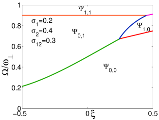
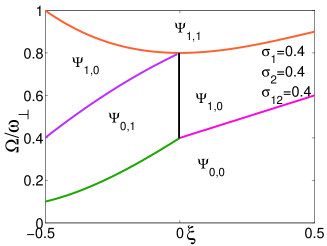
(a) (b)

Figure 1: (color online) Ground-state phase diagrams with different choices of the parameters for a rotating BEC in the presence of gauge potentials in the $\xi$-$\Omega/\omega_{\bot}$ plane. The boundaries separating different phases are plotted. $\sigma_{i}$, $\sigma_{12}$, $\Omega/\omega_{\bot}$ and $\xi$ are all dimensionless quantities.

For sufficiently weak interactions, the energy of atoms in the rotating frame is minimized when the wave functions $\Psi_{1}$, $\Psi_{2}$ are composed of only one component, respectively, i.e., $\Psi_{m_{1},m_{2}}=$ $(r^{m_{1}}e^{im_{1}\varphi}e^{-r^{2}/2a_{1}^{2}},r^{m_{2}}e^{im_{2}\varphi}e^{-r^{2}/2a_{2}^{2}})^{T}$ Jackson . In this case the energy of the system becomes

$$\mathcal{E}_{m_{1},m_{2}} = (1-\frac{\Omega}{\omega_{\bot}})\Bigl{[}m_{1}+1+\frac{m_{2}+1}{1-\xi}\Bigr{]}$$ (37)

$$+\sigma_{1}\frac{(2m_{1})!}{2^{2m_{1}}(m_{1}!)^{2}}+\sigma_{2}(1-\xi)\frac{(2m_{2})!}{2^{2m_{2}}(m_{2}!)^{2}}$$

$$+\sigma_{12}\frac{(m_{1}+m_{2})!(1-\xi)^{(m_{2}+1)}}{2^{m_{1}+m_{2}-1}m_{1}!m_{2}!},$$

in unit of $\hbar\omega_{\bot}$. Here $\xi\equiv\gamma\big{/}(M\omega_{\bot})$, $\sigma_{i}\equiv a_{si}N\big{/}Z$ and $\sigma_{12}\equiv a_{s12}N\big{/}Z$. For definite values of $\Omega$ and $\xi$, the energy of the system depends on the quantum numbers $m_{1}$ and $m_{2}$. The optimal values of $m_{1}$ and $m_{2}$ corresponding to the ground state can be determined by minimizing the energy Eq. (37).

From Eq. (37) we can see that $\mathcal{E}_{1,0}$ and $\mathcal{E}_{0,1}$ become lower than $\mathcal{E}_{0,0}$ at critical frequencies of rotation given by

$$\frac{\Omega_{1,0}}{\omega_{\bot}} = 1-\frac{\sigma_{1}}{2}-(1-\xi)\sigma_{12},$$

$$\frac{\Omega_{0,1}}{\omega_{\bot}} = 1-\frac{(1-\xi)^{2}\sigma_{2}}{2}-\sigma_{12}(1+\xi)(1-\xi)^{2},$$ (38)

respectively. The vortex begins to be created in one component of the system when the frequency of the rotation reaches the minimal value of {$\Omega_{1,0}$, $\Omega_{0,1}$}. For some values of $\xi$, vortices can be created in both components of the system when $\Omega$ reaches some critical value $\Omega_{m_{1},m_{2}}$. Thus the state $\Psi_{m_{1},m_{2}}$ with $m_{1}$ and $m_{2}$ being both larger than zero becomes more favorable in energy for $\Omega\geq\Omega_{m_{1},m_{2}}$. This critical frequency $\Omega_{m_{1},m_{2}}$ can be calculated from the two conditions,

$$\mathcal{E}_{m_{1},m_{2}}-\mathcal{E}_{m_{1}-1,m_{2}}=0,\quad\mathcal{E}_{m_{1},m_{2}}-\mathcal{E}_{m_{1},m_{2}-1}=0.$$

Thus we can plot out the ground-state phase diagram of the rotating BEC in which the boundaries between different phases are obtained by the relation $\mathcal{E}_{m_{1},m_{2}}-\mathcal{E}_{m^{\prime}_{1},m^{\prime}_{2}}=0$. Fig. 1 is plotted for two different choices of the parameters where the $\sigma$’s are small in order to satisfy the assumption of weak interactions. One can see that the shapes of the phase diagram for the two parameter choices change distinctly. This is due to the differences of the scattering lengths can break the spatial symmetry of the ground state. From Fig. 1, we can find the angular momentum of the system depends not only on the rotating frequency $\Omega$ but also on the strength of the gauge potential for given interactions. Discontinuous transitions may be observed through changing the value of $\xi$ even if $\Omega$ is a constant. The presence of gauge potentials makes the phase diagram of the system much richer.

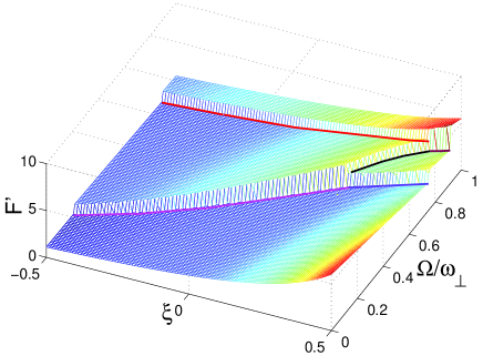
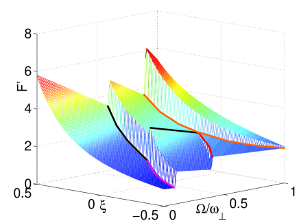
(a) (b)

Figure 2: (color online) The curve surfaces are the derivatives (in the unit of $\hbar\omega_{\bot}$) of the ground-state energy along $(1,-1)$ direction versus $(\xi,\Omega/\omega_{\bot})$ for parameters $\sigma_{1}=0.2,\sigma_{2}=0.4,\sigma_{12}=0.3$ (top panel) and $\sigma_{1}=\sigma_{2}=\sigma_{12}=0.4$ (bottom panel) respectively. The discontinuous steps precisely occur at boundaries separating different phases illustrated in Fig. 1.

Since we have the expressions of the energy levels near the ground state, the phase diagram can be verified with the help of the derivative of the ground-state energy. In Fig. 2, we plot the derivative of the ground-state energy along the $(1,-1)$ direction versus $(\xi,\Omega/\omega_{\bot})$,

$$F^{\prime}(\xi,\Omega)=\frac{\partial\mathcal{E}_{g}}{\partial\xi}-\frac{\partial\mathcal{E}_{g}}{\partial(\Omega/\omega_{\bot})},$$ (39)

where $\mathcal{E}_{g}$ is the ground-state energy of the system. One can see that discontinuous steps emerge in the $F^{\prime}(\xi,\Omega)$ surface (i.e., singularities for the derivative of $F^{\prime}(\xi,\Omega)$). This exhibits the boundaries separating different phases as it is also an effective quantity to characterize quantum phase transitions Wu . These boundaries indeed concise with those given in Fig. 1. As well known, there are various quantities for characterizing quantum phase transitions, such as the quantum entanglement Osterloh-etc and the fidelity Zanardi . The former is convenient if the reduced density matrix for paring correlation is computable while the latter is convenient if the ground state is expressible. In present case, the derivative of the ground-state energy is the most convenient quantity for that purpose.

The above discussion is based on the assumption of weak interactions, which requires that the interaction energy must be relatively much smaller than kinetic and trapping potential energies for each component. The former is of order $\sim\rho_{i}g_{i}$ (i=1,2), and the latter is of order $\sim\hbar\omega_{i}$, where $\rho_{i}$ is the particle density of the $i$th component in the $x$-$y$ plane. The cross section of the $i$th component is $\pi a_{i}^{2}$ in the weak interaction limit. Thus, the density $\rho_{i}$ is $~{}1/\pi a_{i}^{2}$. So we can obtain the effective coupling constant $\sigma_{i}\ll 1$ from the condition $\rho_{i}g_{i}\ll\hbar\omega_{i}$.

If the value of $\sigma_{i}$ violates the condition of weak interactions, the energy of the system will be minimized when many components in the expansion of Eq. (33) contribute to the wave function $\Psi_{i}$. In this case, the equations (IV) is still valid. To calculate the expectation value of $r_{i}^{2}$ and interaction Hamiltonian $H_{int}$ given in Eq. (IV), the numerical simulation and the averaged vortex approximation Ho are efficient methods. Note that two sets of vortex lattices may be formed in this case. The structure of vortex lattices depends on the strength of interactions as well as that of the gauge potentials. The presence of gauge potentials can increase the diversity of vortex-lattice structures, so it is worthwhile to further study these systems.

V Conclusion

In summary, we have given a general description of the dark states and found that $N-1$ degenerate dark states can be generated with the help of $N$ laser fields coupling $N$-fold degenerate ground states with a common exited state. Interferences between two waves with different frequencies can produce such radiation fields that their amplitudes are not only spatially dependent but also time-dependent. They can induce vector and scalar gauge potentials. As an example, we have considered a tripod system for which one can obtain a time-periodic gauge potential using a specific laser field. We have given a configuration of laser field that leads to a uniform $U(2)$ magnetic field, in which we have discussed the features of Landau levels and studied the quantum phase transitions of a rotating BEC using the derivative of the ground-state energy. We have shown that the presence of gauge potentials will make the picture of rotating BECs to be much richer.

This work is supported by NSFC No. 10225419 and No. 10674117.

References

(1)
K. W. Madison, F. Chevy, W. Wohlleben and J. Dalibard, Phys. Rev.
Lett. 84, 806 (2000).
(2)
M. V. Berry, Proc. R. Soc. A 392, 45 (1984).
(3)
F. Wilczek and A. Zee, Phys. Rev. Lett. 52, 2111 (1984).
(4)
G. Juzeliunas and P. Öhberg, Phys. Rev. Lett. 93, 033602
(2004).
(5)
G. Juzeliunas and P. Öhberg, J. Ruseckas, and A. Klein, Phys.
Rev. A 71, 053614 (2005).
(6)
P. Öhberg, G. Juzeliunas, J. Ruseckas, and M. Fleischhauer,
Phys. Rev. A 72, 053632 (2005)
(7)
D. Jaksch and P. Zoller, New. J. Phys. 5, 56 (2003).
(8)
P. Zhang, Y. Li and C. P. Sun, Eur. Phys. J. D 36, 229
(2005)
(9)
R. Dum and M. Olshanii, Phys. Rev. Lett. 76, 1788 (1996).
(10)
K. Osterloh, M. Baig, L. Santos, P. Zoller, and M. Lewenstein,
Phys. Rev. Lett. 95, 010403 (2005).
(11)
J. Ruseckas, G. Juzeliunas, P. Ögberg and M. Fleischhauer,
Phys. Rev. Lett. 95, 010404 (2005).
(12)
M. Fleischhauer and M. D. Lukin,
Phys. Rev. Lett. 84, 5094 (2000);
Phys. Rev. A 65, 022314 (2002).
(13)
P. Q. Jin, Y. Q. Li and F. C. Zhang,
J. Phys. A: Math and Gen, 39, 7115 (2006).
(14)
A. D. Jackson and G. M. Kavoulakis, Phys. Rev. A 70, 023601
(2004).
(15)
L.-A. Wu, M. S. Sarandy, and D. A. Lidar, Phys. Rev. Lett.
93, 250404 (2004).
(16)
A. Osterloh, L. Amico, G. Falci, and R. Fazio, Nature 416, 608 (2002).
S. J. Gu, H. Q. Lin and Y. Q. Li, Phys. Rev. A 68, 042330 (2003).
G. Vidal, J. I. Latorre, E. Rico, and A. Kitaev, Phys. Rev. Lett. 90, 227902 (2003);
(17)
P. Zanardi, M. Cozzini, and P. Giorda, cond-mat/0606130.
(18)
T. L. Ho, Phys. Rev. Lett. 87, 060403 (2001).
(b)
(b)
(b)
(b)