Finite-size Effects in a Two-Dimensional Electron Gas with Rashba Spin-Orbit Interaction

Abstract

Within the Kubo formalism, we estimate the spin-Hall conductivity in a two-dimensional electron gas with Rashba spin-orbit interaction and study its variation as a function of disorder strength and system size. The numerical algorithm employed in the calculation is based on the direct numerical integration of the time-dependent Schrödinger equation in a spin-dependent variant of the particle source method. We find that the spin-precession length, $L_{s}$ controlled by the strength of the Rashba coupling, establishes the critical lengthscale that marks the significant reduction of the spin-Hall conductivity in bulk systems. In contrast, the electron mean free path, inversely proportional to the strength of disorder, appears to have only a minor effect.

I Introduction

The physical phenomenon behind the spin-Hall effect (SHE)Sinova ; Murakami in two-dimensional (2D) systems is the flow of a pure spin current, spin-polarized in a transverse direction, driven by a perpendicular electric field. Its existence is conditioned by the presence of a spin-orbit interaction (SOI), such as Rashba-Dresselhaus Rashba ; Dresselhaus in n-type two dimensional systems or the spin-split band structure in $p$-type GaAs.sH

If in clean samples the spin-Hall conductivity, $\sigma_{sH}$, was predicted to have a universal, constant value of $e/8\pi$, in the presence of disorder the resulting picture was less clear. It was pointed out that, in 2D infinite systems, in the presence of short range scatterers, the vertex corrections provided the exact compensation to cancel the effectInoue . Moreover, an argument was made that this cancellation occurs even for infinitesimal disorder potentialsDimitrova . These conclusions were challenged by analyticMurakami2 and numerical calculationsMarinescu1 ; Nikolic ; Shen of the spin-Hall conductivity in one and two-dimensional finite-size mesoscopic samples, performed within the Landauer-Büttiker formalism, where it was shown that the effect survives up to a critical disorder strength.

Even though the robustness of the spin-Hall effect in the presence of disorder seems to have been definitively confirmed by the angle-resolved optical detection of spin polarization at opposite edges of a two dimensional hole layer Wunderlich , a better understanding of the mechanism by which disorder and system size affect spin transport in systems with spin-orbit interaction warrants further investigation. We focus therefore on a study of the interplay between the disorder strength, embodied in the electron mean free path $l$, and the spin precession length $L_{s}$ proportional to the spin-orbit interaction, in determining the spin-transport regime in finite size samples. Such an analysis is especially relevant in two dimensions where, in the absence of any additional interactions, the two lengths are independent of each and along with the Fermi energy are the only relevant physical parameters of the system.

The relationship between $l$ and $L_{s}$ and the system size, $L$, determines the existence of four distinctive transport regimes. A semi-classical approximation is appropriate for $L_{s}\ll L$, when the spin coherence is lost over the length of the sample, while $L_{s}\gg L$ corresponds to a mesoscopic regime. When $l\gg L$ the electron propagation is ballistic, while for $l\ll L$ multiple scattering events are assumed and the diffusive regime is present.

In the following analysis, we use the Kubo formula to estimate $\sigma_{sH}$ as a function of system size and disorder in a two-dimensional electron system. The numerical formalism adopted here represents an extension to the spin-Hall problem of the particle-source method, developed by TanakaTanaka . This algorithm is based on the direct integration of the time dependent Schrödinger equation and allows the calculation of the matrix elements of the Green’s functions, linear response functions, or any combinations of Green’s function and quantum operators in a very efficient way.

The main result of this paper is that the delimitation between the mesoscopic and semiclassical regimes, as reflected by the rapid decline of the spin-Hall conductivity, is established by $L_{s}$. For system sizes smaller than $L_{s}$ the spin Hall conductivity increases monotonically with the system size, while being weakly affected by disorder. When $L\gg L_{s}$, $\sigma_{sH}$ decreases exponentially for any amount of disorder in the system. This result supports the conclusions of two previous reports by Sheng et al. Sheng and Nomura et al. Nomura where it was found that $\sigma_{sH}$ remains finite up to an, unspecified, characteristic length scale and vanishes in the thermodynamic limit for any small amounts of disorder in the system. Here, we identify this length as being determined by the spin-precession length. Our results reflect no qualitative modification of the overall behavior when the system evolves from the ballistic to the diffusive regimes, crossover controlled by the mean free path characteristic lengthscale. For a fixed Fermi energy and $L_{s}$, the spin-Hall conductivity decrease monotonically with disorder for any system size, as the system evolves from diffusive to ballistic regime.

II Theoretical Framework

II.1 Model

The single-particle Hamiltonian that describes the dynamics of an electron of momentum $\mathbf{p}$ and effective mass $m^{*}$, is written, in terms of the Pauli matrices $\sigma_{x,y}$ and the Rashba coupling constant $\lambda$, as:

$${\tilde{H}}=\frac{{\mathbf{p}}^{2}}{2m^{*}}+\lambda\left(\sigma_{x}p_{y}-\sigma_{y}p_{x}\right).$$ (1)

The exact diagonalization procedure that can be performed on the Hamiltonian in the case of a clean systemSinova , becomes impossible when disorder is included in the form of an additional random scattering term. It is therefore more convenient, for a numerical analysis, to adopt the tight-binding approximation for the many-body Hamiltonian, by employing a local orbital basis associated with a virtual square $N\times N$ lattice, of constant $a_{0}$. In this model, the many-body Hamiltonian, is:

$$H = \sum\limits_{i,\alpha}\varepsilon_{i}c_{i\alpha}^{\dagger}c_{i\alpha}-t\sum\limits_{<i,j>,\alpha}c_{i\alpha}^{\dagger}c_{j\alpha}$$

$$+ V_{R}\sum\limits_{i,\delta_{x},\delta_{y}}\left[\left(c_{i\uparrow}^{\dagger}c_{i+\delta_{x}\downarrow}-c_{i\downarrow}^{\dagger}c_{i+\delta_{x}\uparrow}\right)\right.$$

$$-i\left.\left(c_{i\uparrow}^{\dagger}c_{i+\delta_{y}\downarrow}+c_{i\downarrow}^{\dagger}c_{i+\delta_{y}\uparrow}\right)\right].$$

In this expression, an electron with spin $\alpha$ at site $i$, created by $c_{i\alpha}^{\dagger}$, is subjected to a random on-site energy as in the Anderson model for disorder, generated by a box distribution $\varepsilon_{i}\in[-W/2,W/2]$. The electron transport is described by a sequence of discrete hopping events. Lateral transport, without spin flip, to an adjacent site occurs with probability $t=\hbar^{2}/2m^{*}a_{0}$, taken to be the unit of energy in our calculation, as described by the second term in Eq. (II.1). Propagation along the diagonal sites, driven by the spin-orbit interaction, occurs with a simultaneous spin-flip, as in the last term of Eq. (II.1). The latter is most important as it mixes the spin channels and leads to a finite spin-Hall conductivity and spin accumulations at the edges of sample. The Rashba coupling constant is renormalized by the lattice constant to $V_{R}=\hbar\lambda/a_{0}$.

The Kubo formula for the spin-Hall conductivity is written as:

$$\sigma_{sH}=\frac{1}{2}\,{\rm Tr}\int\frac{d\varepsilon}{2\pi}\left(-\frac{\partial f(\varepsilon)}{\partial\varepsilon}\right)\left<{j}_{x}^{z}\left[{G}_{R}(\varepsilon)-{G}_{A}(\varepsilon)\right]\right.$$

$$\left.\times\,{v}_{y}\,{G}_{A}(\varepsilon)-{j}_{x}^{z}\,{G}_{R}(\varepsilon)\,{v}_{y}\left[{G}_{R}(\varepsilon)-{G}_{A}(\varepsilon)\right]\right>$$ (3)

The velocity operator is defined by the commutator: $i\,\hbar v_{y}=\left[y,H\right]$, while for the spin current we adopt a traditional expressionNiu given in terms of the anticommutator between the velocity operator and the Pauli matrix $\sigma_{z}$: $j_{x}^{z}=\hbar\left\{\sigma_{z},v_{x}\right\}/4$. $G_{R/A}(\epsilon)$ represents the retarded/advanced Green’s function. In Eq. (3) the integration over the energy is restricted over the Fermi surface due to the presence of $\left[-\partial f(\varepsilon)/\partial\varepsilon\right]$ factor.

In the tight-binding framework, the effect of disorder and spin-orbit interaction strength on the spin Hall conductance was investigated previously, using the Landauer-Büttiker formalismHankiewicz ; Nikolic2 . As will be discussed in the next section, in the present work we use a different approach for computing the Green’s function needed for the calculation of the spin-Hall conductivity.

II.2 Numerical algorithm

Since the purpose of this investigation is an analysis of the spin-Hall conductivity dependence on system size and disorder, we will apply the Kubo formula to large size systems for different values of the disorder potential W. The numerical algorithm that underlies this calculation has been introduced in Ref. Tanaka, and represents an extension of the particle-source method combined with tight-binding formalism. This method was first applied to the calculation of the Green’s function, density of states, conductivity Iitaka1 and Hall conductivityTanaka . The main advantage is that one can evaluate both the diagonal and off-diagonal parts of the Green’s function and their products with other quantum operators with a low computing effort. In principle the computing effort for computing the Green’s function is $O(N^{3})$, (Hamiltonian is expressed as a $N\times N$ matrix) while within the present algorithm only $O(N)$ computational effort is required for the same calculation. Here, we briefly outline the main features of the algorithm.

The central part of the method consists in solving the time dependent Schrödinger equation with a single-frequency source term:

$$i\hbar\frac{d\,\left|\tilde{j},t\right>}{d\,t}=H\left|\tilde{j},t\right>+\left|j\right>\theta(t)\exp^{-i(E+i\eta)t}\;,$$ (4)

where $\eta$ is a finite small value and $\theta$ is the step function. The solution of the equation, with the initial condition $\left|\tilde{j},t=0\right>=0$ becomes:

$$\left|\tilde{j},t\right> = -i\int_{0}^{t}dt^{\prime}e^{-iH(t-t^{\prime})}\left|{j}\right>e^{-i(E+i\eta)t^{\prime}}$$

$$= \frac{1}{E+i\eta-H}[e^{-i(E+i\eta)t}-e^{-iHt)}\left|{j}\right>\;.$$

For sufficiently large time, one can then write the solution to the Schrödinger equation in terms of the Green’s function acting on the ”source” $\left|j\right>$ with the relative accuracy $\delta=e^{-\eta T}$, as:

$$\left|\tilde{j},T\right>=G(E+i\eta)\left|{j}\right>e^{-i(E+i\eta)T}\;,$$ (6)

leading to a Green’s function operating on the ket $\left|{j}\right>$:

$$G(E+i\eta)\left|{j}\right>=\lim_{T\rightarrow\infty}\left|\tilde{j},T\right>e^{i(E+i\eta)T}\;.$$ (7)

The matrix element between states $\left<i\right|$ and $\left|j\right>$ is then obtained as:

$$\left<i\right|G(E+i\eta)\left|j\right>=\lim_{T\rightarrow\infty}\left<i\right|\left.\tilde{j},T\right>\;.$$ (8)

The matrix elements of a product including several Green’s functions and other operators are obtained by choosing a new initial state, such as $\left|j^{\prime}\right>=AG(E+i\eta)\left|j\right>$ in Eq. (4) and repeating the same procedure.

To calculate the matrix elements of the Green’s function at many different energy values, one solves Eq. (4) simultaneously for a source term with multiple frequencies, $\left|j\right>\left(\sum_{l}e^{-i(E_{l}+i\eta)t}\right)\theta(t)$. Following the algorithm outlined above, one obtains as an approximate solution, the ket

$$\left|\tilde{j},T\right>\simeq\sum_{l}G(E_{l}+i\eta)\left|j\right>e^{-i(E_{l}+i\eta)T}.$$ (9)

The matrix element of the Green’s function between the states $\left<i\right|$ and $\left|j\right>$ for a giver energy is then easily obtained as

$$G_{ij}(E_{l}^{\prime}+i\eta) = \left<i\right|G(E_{l}^{\prime}+i\eta)\left|j\right>$$ (10)

$$= \frac{1}{T}\int_{0}^{T}dt^{\prime}\left<i|\tilde{j},t^{\prime}\right>e^{i(E_{l^{\prime}}+i\eta)t^{\prime}}\;,$$

where the terms involving transitions between different energies have been neglected with the relative accuracy $\delta=1/T\Delta E$, with $\Delta E$ the minimum increment in the energies $E_{l}$.

To obtain the time dependent ket $\left|\tilde{j};T\right>$, a direct numerical integration of the Schrödinger equation can be performed, as in the ”leap-frog” algorithmIitaka . This is a second order, symmetrized differencing scheme, accurate up to $(H\Delta t)^{2}$. In this form, Eq. (4) becomes:

$$\left|\tilde{j};t+\Delta t\right> = -2i\Delta tH\left|\tilde{j};t\right>+\left|\tilde{j};t-\Delta t\right>$$

$$- 2i\Delta t\left|j\right>\sum_{l}e^{-i(E_{l}+i\eta)t}\theta(t)\;,$$

with a time step $\Delta t$ determined by $\Delta t=\beta/E_{max}$, where $E_{max}$ is the absolute value of the extreme eigenvalue and $\beta$ is a parameter whose value is less than 1 in order for the solution to be stableAskar .

Estimating the trace in Eq. (3) requires a suitable basis set, such as the local orbital basis. It is more efficient however, to choose a randomized version of this basis, described by a ket $\left|\phi\right>=\sum_{n=1}^{N}\left|n\right>\exp(-i\,\phi_{n})$, where $\left|n\right>$ are the tight-binding orbitals and $\phi_{n}$ are random numbers in the $\left[0,2\pi\right]$ interval. For a given operator $A$, $\left<\phi\right|A\left|\phi\right>\simeq\sum_{n}\left<n\right|A\left|n\right>$ within the statistical errors of $1/\sqrt{N}$.

III Results and Discussion

In this section we show the results of our computation based on the previously outlined algorithm. First, we study the Fermi energy dependence of the spin-Hall conductivity, presented in Fig. 1. Random Fermi energies in the interval [-4t,4t] were considered and we average over 2000 samples, for each system size. For clean systems and for states in the band, $\sigma_{sH}$ is close to 0.8 (in unit of $e/8\pi$), except at half filling where due to electron-hole symmetry considerations it vanishes. In the presence of disorder, the calculated value of $\sigma_{sH}$ decreases, our results reproducing very well the known behavior previously obtained in the Landauer-Büttiker formalismNikolic ; Marinescu1 or by the analytical Kubo formulaNomura .

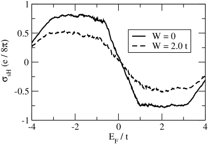
Figure 1: Spin Hall conductivity as function of Fermi Energy in units of $e/8\pi$, for clean and disordered systems. System size is 30$\times$ 30. Spin-orbit interaction strength is fixed to $V_{R}=0.2\,t$. Average was done over 2000 random frequencies.

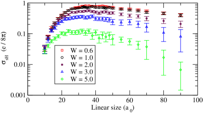
Figure 2: Spin Hall conductivity as function of system size in units of $e/8\pi$ represented on a logarithmic scale. Fermi energy is fixed to $E_{F}=-3.0\;t$ and the spin precession length is $L_{s}\simeq 16a_{0}$, corresponding to $V_{R}=0.2\,t$. Mean free path ranges from $l\simeq 45a_{0}$ for $W=0.6\;$ down to a few lattice constants when disorder increases. Averages are done over $10^{3}$ disorder samples and for each, 200 initial state vectors are considered.

The dependence of the spin-Hall conductivity on the system size is shown in Fig. 2. One is interested in finding whether the variation of $\sigma_{sH}$ is dramatically changed by disorder and what is the length scale at which this change occurs. For this, the two relevant parameters are the electronic mean free path $l$ and the spin-precession length $L_{s}$. In a quasi-classical approximation $l=12\hbar v_{F}a_{0}/(2\pi N(E_{F})\,W)^{2}$ , where $v_{F}$ is the Fermi velocity, while $N(E_{F})$ is the density of states at the Fermi energy measured from the bottom of the band. The spin-precession length is defined in terms of the Rasba coupling constant by $L_{s}=\pi ta_{0}/V_{R}$.

The electronic mean free path is the lengthscale that separates the ballistic from the diffusive regimes, with a ballistic behavior for system sizes smaller than $l$ and diffusive otherwise. We found that the crossover between these two regime is smooth, without any dramatic changes in the overall behavior of the spin-Hall conductivity. The only observable effect is a decrease of the spin-Hall conductivity when disorder increases. For example, when $W=0.6\;t$, $l\simeq 45\;a_{0}$, while for $W=1.0\;t$, $l\simeq 16\;a_{0}$, whereas, as can be seen in Fig. 2, the behavior of the spin-Hall conductivity remains unchanged. At the same time, for system sizes below $L_{s}$, $\sigma_{sH}$ is always monotonically increasing, reaches a plateau between $L_{s}$ and $2L_{s}$, and then decreases for large system sizes, being expected to vanish in the thermodynamic limit, as in Refs.Sheng ; Nomura . The spin-precession length, therefore, is the characteristic lengthscale at which a crossover between the different regimes of the spin-Hall conductivity is expected.

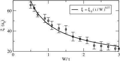
Figure 3: Disorder dependence of the characteristic length scale $\xi$ for Fermi energy $E_{F}=-3.0\,t$ and spin-orbit interaction strength $V_{R}=0.2\,t$.

In the semiclassical regime, a scaling analysis is appropriate. We find that, for a given Fermi energy, the size dependence of the spin-Hall conductivity can be very well fitted with a exponential function $\sigma_{sH}\simeq\exp(-L/\xi)$ where $\xi$ is a characteristic length that depends on the disorder strength, being divergent in a clean system. In Fig. 3 we present the dependence of this characteristic length as function of disorder which follows a power law $\xi\simeq\xi_{0}\left(t/W\right)^{0.57}$ behavior, with the best fit $\xi_{0}\simeq 46\,a_{0}$. We remark again that the system size where $\sigma_{sH}$ starts to decrease is strongly conditioned by $L_{s}$, rather than $l$ as can be inferred from the similarities between the behaviors drawn for different values of the disorder for the same $L_{s}$. In all our calculations the decrease in the spin-Hall conductivity starts for system sizes $L\simeq 2\,L_{s}$ regardless of the value of the electronic mean free path.

IV Conclusions

In this work we study the effect of the spin-precession length scale and of the electronic mean free path on the the spin-Hall conductivity in different regimes, by adapting the particle-source algorithm to spin transport in systems with SOI in the framework of the the tight-binding approximation. The dependence of $\sigma_{sH}$ on the Fermi energy is also investigated. Our main finding is that the spin precession length is the critical length scale for the spin-Hall behavior. For a system size smaller that $L_{s}$, the spin-Hall conductivity increases even in the presence of disorder, reaches a plateau between $L_{s}$ and $2\,L_{s}$ and then in the semiclassical limit, when $L\gg L_{s}$ decreases exponentially. In the thermodynamic limit, $\sigma_{sH}$ is zero for any amount of disorder present in the system. We have also showed that the electronic mean free path does not play a fundamental role in the spin-Hall conductivity behavior.

Acknowledgments. This research was supported by the Hungarian Grants OTKA Nos. NF061726 and T046303, and by the Romanian Grant CNCSIS 1.97.

References

- (1) J. Sinova, D. Culcer, Q. Niu, N.A. Sinitsyn, T. Jungwirth and A.H. MacDonald, Phys. Rev. Lett. 92, 126603 (2004).
- (2) S. Murakami, Phys. Rev. B 69, 241202(R) (2004);
- (3) E.I. Rashba, Sov. Phys. Solid State 2, 1109 (1960); M.I. Dyakonov and V.I. Perel, Sov. Phys. JETP 33, 1053 (1971).
- (4) G. Dresselhaus, Phys. Rev. 100, 580, (1955).
- (5) J. Schliemann and D. Loss, Phys. Rev. B 69, 165315 (2004); B.A. Bernevig, J. Hu, E. Mukamel, and S.-C. Zhang, Phys. Rev. B 70, 113301 (2004); B.A. Bernevig and S.-C. Zhang, Phys. Rev. B 72, 115204 (2005); E.I. Rashba, Phys. Rev. B 68, 241315 (2003); L. Hu, J. Gao and S.-Q. Shen, Phys. Rev. B 68, 153303, (2003); A.A. Burkov, A.S. Nunez and A. H. MacDonald, Phys. Rev. B 70, 155308 (2004).
- (6) J .I. Inoue , G. E. W. Bauer and L. W. Molenkamp, Phys. Rev. B 70, 041303(R) (2004).
- (7) O. V. Dimitrova, Phys. Rev. B 71, 245327 (2005).
- (8) Naoyuki Sugimoto, Shigeki Onoda, Shuichi Murakami, Naoto Nagaosa, Phys. Rev. B 73, 113305 (2006).
- (9) C.P. Moca and D.C. Marinescu, Phys. Rev. B 72, 165335 (2005).
- (10) B. K. Nikolić, S. Souma L. Zârbo and J. Sinova, Phys. Rev. Lett. 95, 046601 (2005).
- (11) S.-Q. Shen, M. Ma, X.C. Xie, and F.C. Zhang, Phys. Rev. Lett. 92, 256603 (2004);
- (12) J. Wunderlich, B. Kaestner , J. Sinova and T. Jungwirth, Phys. Rev. Lett. 94, 047204 (2005).
- (13) H. Tanaka and M. Itoh, Phys. Rev. Lett. 81, 3727 (1998).
- (14) D. N. Sheng, L. Sheng, Z. Y. Weng and F. D. M. Haldane, Phys. Rev. B 72, 153307 (2005).
- (15) K. Nomura, J. Sinova, N. A. Sinitsyn and A. H. MacDonald, Phys. Rev. B 72, 165316 (2005) K. Nomura, J. Wunderlich, J. Sinova, B. Kaestner, A. H. MacDonald and T. Jungwirth, Phys. Rev. B 72, 245330 (2005).
- (16) K. Nomura, Jairo Sinova, T. Jungwirth, Q. Niu, A. H. MacDonald, Phys. Rev. B 71, 041304 (2005).
- (17) E. M. Hankiewicz, L. W. Molenkamp, T. Jungwirth and Jairo Sinova, Phys. Rev. B 70, 241301(R) (2004)
- (18) B. K. Nikolić, Liviu P. Zârbo, and S. Souma, Phys. Rev. B 72, 075361 (2005)
- (19) T. Iitaka Riken Super Computing Prog. Rep, 1, 1 (1996); T. Iitaka, S. Nomura, H. Hirayama, X. Ahao, Y. Aoyagi and T. Sugano, Phys. Rev. E 56, 1222 (1997); H. Tanaka, Phys. Rev. B 57, 2168 (1998).
- (20) T. Iitaka, Phys. Rev. E 49, 4684 (1994).
- (21) A. Askar and A. S. Cakmak, J. Chem. Phys. 68, 2794 (1978).