Activity patterns on random scale-free networks: Global dynamics arising from local majority rules

Abstract

Activity or spin patterns on random scale-free network are studied by mean field analysis and computer simulations. These activity patterns evolve in time according to local majority-rule dynamics which is implemented using (i) parallel or synchronous updating and (ii) random sequential or asynchronous updating. Our mean-field calculations predict that the relaxation processes of disordered activity patterns become much more efficient as the scaling exponent $\gamma$ of the scale-free degree distribution changes from $\gamma>5/2$ to $\gamma<5/2$. For $\gamma>5/2$, the corresponding decay times increase as $\ln(N)$ with increasing network size $N$ whereas they are independent of $N$ for $\gamma<5/2$. In order to check these mean field predictions, extensive simulations of the pattern dynamics have been performed using two different ensembles of random scale-free networks: (A) multi-networks as generated by the configuration method, which typically leads to many self-connections and multiple edges, and (B) simple-networks without self-connections and multiple edges. We find that the mean field predictions are confirmed (i) for random sequential updating of multi-networks and (ii) for both parallel and random sequential updating of simple-networks with $\gamma=2.25$ and $\gamma=2.6$. For $\gamma=2.4$, the data for the simple-networks seem to be consistent with mean field theory as well whereas we cannot draw a definite conclusion from the simulation data for the multi-networks. The latter difficulty can be understood in terms of an effective scaling exponent $\gamma_{\rm eff}=\gamma_{\rm eff}(\gamma,N)$ for multi-networks. This effective exponent is determined by removing all self-connections and multiple edges; it satisfies $\gamma_{\rm eff}\geq\gamma$ and decreases towards $\gamma$ with increasing network size $N$. For $\gamma=2.4$, we find $\gamma_{\rm eff}\mathrel{\mathchoice{\vbox{\offinterlineskip\halign{\hfil$\displaystyle#$\hfil\cr>\cr\sim\cr}}}{\vbox{\offinterlineskip\halign{\hfil$\textstyle#$\hfil\cr>\cr\sim\cr}}}{\vbox{\offinterlineskip\halign{\hfil$\scriptstyle#$\hfil\cr>\cr\sim\cr}}}{\vbox{\offinterlineskip\halign{\hfil$\scriptscriptstyle#$\hfil\cr>\cr\sim\cr}}}}5/2$ up to $N=2^{17}$.

I Introduction

Both the overall topology and the local structure of complex networks influence the efficiency as well as the robustness or sensitivity of dynamic processes occurring on these networks. Furthermore, the local network architecture often evolves with time in order to optimize certain network properties. This interplay of structure and dynamics eventually leads to the formation of highly optimized network topologies for specific dynamic processes.

Understanding the underlying mechanism for the optimization of networks via evolution is an important but challenging problem of current network research. There are two major difficulties. First, the optimization of different dynamic processes may require different network architectures. For example, we would not be surprised to find out that the architectures of car traffic networks and electronic networks on micro-processor chips are rather different. Therefore in order to study network evolution, we should focus on a particular dynamic process. Second, the evolution process is usually governed by some more or less complex growth rules which are coupled in some unknown way to the dynamic process under consideration.

In this article, we use a somewhat different approach and study the influence of network architectures on relatively simple dynamic processes. By performing such an analysis, we are able to identify those aspects of the network structure that are important for the dynamic processes. Such a theoretical investigation should also be useful to analyze the available empirical data about complex networks in terms of optimization to design improved network structrues for a particular dynamic process.

A network can be represented by a graph of vertices (nodes) and edges (links). Each edge of the network connects two vertices of the network. The vertex degree $k$ is equal to the total number of edges that are connected to this vertex. Recent structural studies on complex networks Albert and Barabási (2002); Dorogovtsev and Mendes (2002); Newman (2003) show that the topology of real-world networks often has the so-called scale-free property Barabási and Albert (1999). This means that the total number $N(k)$ of vertices with degree $k$ scales with $k$ as a power-law, $N(k)\sim k^{-\gamma}$, with the decay or scaling exponent $\gamma$. Such a power-law scaling of the degree distribution appears if the network grows via a preferential attachment mechanism Barabási and Albert (1999). It is also plausible that the scale-free scaling is a result of network evolution and optimization, but so far there are only a few theoretical studies that have addressed this issue (e.g., Refs. Valverde et al. (2002); Ferrer i Cancho and Solé (2003); Variano et al. (2004); Wang et al. (2005)).

In the following, we will consider the influence of scale-free random networks on the activity patterns of binary or Ising-like variables which are governed by local majority-rule dynamics. We focus on scale-free networks because they are abundant in our biosphere. We study local majority-rule dynamics because it is simple and frequently encountered in the real world, and also because it can be readily extended to a large class of more complicated dynamic processes.

We perform both analytical mean-field calculations and extensive numerical simulations on these model systems. Our mean-field calculations predict that, when the scaling exponent $\gamma$ of the substrate network changes from $\gamma>5/2$ to $\gamma<5/2$, a qualitative improvement in the efficiency of the dynamic process can be achieved, namely the typical relaxation time changes from being proportional to $\ln(N)$ to being independent of $N$, where $N$ is the total number of nodes in the network. In the simulations, we consider two different methods to generate ensembles of random scale-free networks: (i) multi-networks, which are generated using the so-called configuration model and contain some multiple edges and self-connections; and (ii) simple-networks, which involve some random reshuffling of edges and do not contain any multiple edges or self-connections. Our mean-field results are quantitatively confirmed by the simulations for simple-networks whereas the behavior on multi-networks exhibits strong finite-size corrections arising from the presence of multiple edges and self-connections. We use both parallel (or synchronous) and random sequential (or asynchronous) updating and find that both updating methods give very similar results for simple-networks whereas they lead to somewhat different results for multi-networks. The present study extends our previous work in Ref. Zhou and Lipowsky (2005) in which we focussed on parallel updating for multi-networks.

Our mean-field theory can be extended to related dynamic processes. Instead of Ising-like variables, we have studied Potts-like variables which can attain three or more different states. We have also considered more complex dynamic rules for which one applies the local majority rule to each spin variable with a certain probaility say ${\cal P}$, and another dynamic rule such as random Boolean dynamics with probability $1-{\cal P}$. Likewise, we have extended our analysis to majority rule dynamics on directed networks and to Hopfield models on scale-free networks Zhou and Lipowsky (2005). In all cases, the mean-field theorey predicts that the dynamic behavior changes qualitatively as one crosses the boundary value $\gamma=5/2$. It is of interest to note that many scale-free networks are characterized by scaling exponents $\gamma$ which fall into the narrow range $2<\gamma\leq 5/2$ as observed in Ref. Aldana and Cluzel (2003). Indeed, table II of Ref. Albert and Barabási (2002) contains a list of ten scale-free networks with $2<\gamma<5/2$, one with $\gamma=2.5$, and only three with $2.5<\gamma<3$.

This paper is organized as follows. We first describe our model system in more detail in Sec. II. Then our mean-field analysis is presented in Sec. III. Simulation results of local majority-rule dynamics are discussed in Sec. IV for random multi-networks with multiple edges and self-connections, and in Sec. V for random simple-networks without any such connections. The simulation results for simple-networks are in complete agreement with the mean field predictions whereas we find only partial agreement between the simulation results for multi-networks and mean field theory. We then argue in Sec. VI that the remaining discrepancies can be understood if one characterizes the multi-networks by an effective $N$–dependent scaling exponent $\gamma_{\rm eff}\geq\gamma$. Finally we conclude our work in Sec. VII with a summary and an outlook on related problems.

II Scale-free networks and majority-rule dynamics

In the following, we study local majority-rule dynamics on scale-free random networks. In order to do so, we first describe the ensemble of random networks used in our study and then define the dynamic rules.

II.1 Scale-free degree sequences

We consider an ensemble of random networks. Each network consists of $N$ vertices and edges that connect pairs of vertices. Each vertex $i$ with $i=1,2,\ldots,N$ is connected to $k_{i}\geq k_{0}$ edges where $k_{0}$ represents the minimal value of the vertex degrees $k_{i}$. As in Ref. Zhou and Lipowsky (2005), we will focus on $k_{0}\geq 2$ for which the network has no ‘dangling ends’ and consists of many cycles. We consider an ensemble of random networks that provide realizations of the degree distribution

$$P(k_{i})\propto k_{i}^{-\gamma}\quad{\rm for}\quad k_{i}\geq k_{0}$$ (1)

which is characterized by a power-law decay with scaling exponent $\gamma$. In order to generate such a network ensemble, we treat the vertex degree $k_{i}$ as a random integer variable governed by the degree distribution (1).

In order to generate a single random network with $N$ vertices, we used the following algorithm for generating a vertex degree sequence consisting of $N$ vertex degrees $k_{i}$. We successively draw a random integer $k_{i}$ according to the degree distribution (1). If the drawn vertex degree satisfies $k_{i}\leq N-1$, we add it to our degree sequence. Otherwise, we discard it and draw another $k_{i}$ until we obtain one that fulfills this inequality. Thus, we use the upper cut-off $k_{\rm max}^{(1)}\equiv N-1$ for the vertex degree sequences. This procedure differs slightly from the one that we used previously in Zhou and Lipowsky (2005). In the latter study, we did not discard and redraw the vertex degrees $k_{i}$ with $k_{i}>N-1$ but replaced them by $k_{i}=N-1$. This procedure has the disadvantage that the actual degree distribution corresponding to the generated vertex degree sequence may develop a small peak at $k_{i}=N-1$ for sufficiently small network size $N$. The new algorithm used here avoids this artefact. The choice for the upper cut-off $k_{\rm max}^{(1)}=N-1$ is rather natural since this is the maximal vertex degree for a network without multiple edges and self-connections. Note that we do not use an upper cutoff $k_{\rm max}^{(1)}\sim N^{1/2}$ as in Refs. Catanzaro et al. (2005); Castellano and Pastor-Satorras (2006).

For analytical estimates, it will be useful to define a second upper cut-off, $k_{\rm max}^{(2)}\equiv k_{0}N^{{1\over\gamma-1}}$, for the vertex degree. The latter cut-off was introduced in Cohen et al. (2000) and rederived by different arguments in Zhou and Lipowsky (2005), see Appendix A. The effective upper cut-off for the generated vertex degree sequence is then given by

$$k_{\rm max}\equiv\min\bigl{(}k_{\rm max}^{(1)},k_{\rm max}^{(2)}\bigr{)}=k_{0}N^{{1\over\gamma-1}}$$ (2)

where the last equality applies to $N>k_{0}^{(\gamma-1)/(\gamma-2)}$, and the actual vertex degree distribution for the generated degree sequence is well approximated by

$$P(k_{i})={k_{i}^{-\gamma}/{\cal A}}\quad{\rm for}\quad k_{0}\leq k_{i}\leq k_{\rm max}$$ (3)

with the normalization constant ${\cal A}=\sum k_{i}^{-\gamma}$. In the limit of large $k_{\rm max}$, the degree distribution (3) is normalizable provided $\gamma>1$, and the normalization constant is then given by

$${\cal A}\equiv\sum\limits_{k=k_{0}}^{k_{\rm max}}k^{-\gamma}\approx{k_{0}^{1-\gamma}-k_{\rm max}^{1-\gamma}\over\gamma-1}\ .$$ (4)

The mean vertex degree of the generated degree sequence is

$$\langle k\rangle=\sum\limits_{k=k_{0}}^{k_{\rm max}}kP(k)\approx k_{0}{(\gamma-1)\bigl{(}1-(k_{0}/k_{\rm max})^{\gamma-2}\bigr{)}\over(\gamma-2)\bigl{(}1-(k_{0}/k_{\rm max})^{\gamma-1}\bigr{)}}\ .$$ (5)

The mean vertex degree $\langle k\rangle$ attains a finite limit for large $k_{\rm max}$ provided $\gamma>2$. It behaves as $\langle k\rangle\approx k_{0}$ for large positive $\gamma$, corresponding to a random network with uniform vertex degree $k=k_{0}$. On the other hand, the expression (5) also implies

$$\langle k\rangle\approx k_{0}{\ln(k_{\rm max}/k_{0})\over 1-(k_{0}/k_{\rm max})}\hskip 14.22636pt{\rm for}\;\;\;\;\gamma=2\ ,$$ (6)

which diverges as $\ln k_{\rm max}$ for large $k_{\rm max}$.

II.2 Multi-networks and simple-networks

After one degree sequence $\{k_{1},k_{2},\ldots,k_{N}\}$ has been generated, we attach $k_{i}$ half-edges to vertex $i$. Then we repeatedly crosslink two half-edges into a complete edge of the network, until all half-edges have been used up. In this way, an initial network with the specified degree sequence is created which is then further randomized by performing a certain number of edge switching moves Milo et al. (2003). We use two different ways to implement the crosslinking process and the subsequent switching process which lead to two different ensembles of networks, multi-networks and simple-networks:

(A) Multi-networks: During the initial crosslinking process, two half-edges are randomly chosen from the set of remaining half-edges and are then crosslinked into an edge of the network. During the subsequent randomization or edge switching process, two edges $\langle ij\rangle$ and $\langle kl\rangle$ are randomly chosen from the set of all edges of the network, and they are replaced by two new edges $\langle ik\rangle$ and $\langle jl\rangle$. A network that has been generated in this way will, in general, contain both self-connections and multiple edges Zhou (2002).

(B) Simple-networks: During the initial crosslinking process, we again randomly choose two half-edges from the set of remaining half-edges but crosslink them only into a tentative edge. This tentative edge is only kept if it provides a connection between two different vertices that have not been connected before. Otherwise, the tentative edge is discarded. In this way, we discard all tentative edges that represent self-connections or multiple edges. During the subsequent randomization or edge switching process, we proceed in an analogous manner: (i) we randomly choose two edges $\langle ij\rangle$ and $\langle kl\rangle$ of the network; (ii) we create two new tentative edges $\langle ik\rangle$ and $\langle jl\rangle$; and (iii) we keep these tentative edges only if they do not represent self-connections or multiple edges. Otherwise, we reject this move and keep the old edges $\langle ij\rangle$ and $\langle kl\rangle$. The networks generated in this way are simple in the sense that they contain no self-connections and no multiple edges.

In principle, the network graphs generated by these two procedures could have several disconnected components. In such a situation, the activity pattern would consist of several subpatterns that are disconnected and, thus, evolve independently of each other. The number and size of these components depends primarily on the scaling exponent $\gamma$ and the minimal vertex degree $k_{0}$. In the following, we will discuss ensembles of networks with $2<\gamma<3$ and $k_{0}\geq 5$ . For these parameter values, all multi- and simple-networks that we generated by the procedures (A) and (B) were found to consist of only a single component. Each of these networks is then characterized by a single activity pattern in which all $N$ vertices participate.

So far, we have not distinguished between a network and its most intuitive representation, the corresponding graph with vertices $i$ and (undirected) edges $\langle ij\rangle$. Another general representation is provided by the adjacency matrix $\mathbf{I}$ of the network. Each element $I_{ij}$ of this $N\times N$ matrix counts the number of edges, $m(i,j)$, between vertex $i$ and vertex $j$, i.e.,

$$I_{ij}\equiv m(i,j)\geq 0.$$ (7)

For an undirected graph as considered here, the adjacency matrix is symmetric and $I_{ji}=I_{ij}$. Furthermore, a simple-network without self-connections and multiple edges is characterized by $I_{ii}=0$ and $0\leq I_{ij}\leq 1$ for all vertex pairs $(i,j)$.

II.3 Local majority-rule dynamics

We now place a binary or Ising-like spin $\sigma_{i}=\pm 1$ on each vertex $i$ of the network. Alternatively, we can use the activity variable $\sigma_{i}^{\prime}\equiv(\sigma_{i}+1)/2$ which assumes the values $\sigma_{i}^{\prime}=1$ and 0 corresponding to an active and inactive vertex $i$, respectively. Thus, the spin configuration $\{\sigma(t)\}\equiv\{\sigma_{1}(t),\sigma_{2}(t),\dots,\sigma_{N}(t)\}$ represents the activity pattern on the network at time $t$.

For the dynamics considered here, the time evolution of the spin or activity pattern is governed by the local time-dependent fields

$$h_{i}(t)\equiv{\sum_{j\neq i}}I_{ij}\sigma_{j}+2I_{ii}\sigma_{i}\,.$$ (8)

Because of the adjacency matrix $\mathbf{I}$, the sum contains contributions from all vertices $j$ that are connected to vertex $i$, and this contribution is weighted by the multiplicity $I_{ij}=m(i,j)$ which counts the number of edges between $i$ and $j$. Therefore, the sign of the local field $h_{i}$ is positive and negative if the weighted majority of the nearest neighbor spins is positive or negative, respectively. For multi-networks, the nearest neighbors are weighted with the corresponding edge multiplicity. For simple-networks, all nearest neighbors have the same multiplicity equal to one, and the absence of self-connections implies $I_{ii}=0$ for all vertices $i$.

In the parallel or synchronous version of the local majority-rule dynamics, the discrete time $t$ is increased by $\Delta t\equiv 1$, and the spin or activity pattern at time $t$ is updated simultaneously on all vertices $i$ using the rule

$$\sigma_{i}(t+1) \equiv +1\hskip 14.22636pt{\rm if}\;\;\;\;h_{i}(t)>0\ ,$$ (9)

$$\equiv -1\hskip 14.22636pt{\rm if}\;\;\;\;h_{i}(t)<0\ .$$

In the random sequential or asynchronous version of the local majority-rule dynamics, time $t$ is increased by $\Delta t\equiv 1/N$, a vertex $i$ is randomly chosen, and the spin value $\sigma_{i}$ on this vertex is updated according to

$$\sigma_{i}(t+1/N) \equiv +1\hskip 14.22636pt{\rm if}\;\;\;\;h_{i}(t)>0\ ,$$ (10)

$$\equiv -1\hskip 14.22636pt{\rm if}\;\;\;\;h_{i}(t)<0\ .$$

while the spin values for all the other vertices remain unchanged during this update. In this way, the update of the whole network from time $t$ to time $t+1$ is divided up into $N$ successive substeps.

If the local field $h_{i}(t)=0$ corresponding to an equal number of up and down spins on the nearest neigbor vertices, we choose $\sigma_{i}(t+\Delta t)=+1$ or $-1$ with equal probability both for the parallel update described by (9) and for the random sequential update as given by (10). These local majority rules, which are equivalent to Glauber dynamics Glauber (1963); Bar-Yam and Epstein (2004) at zero temperature, have two fixed points corresponding to the two completely ordered patterns with $\{\sigma(t)\}=\{\sigma^{(-)}\}\equiv\{-1,-1,\dots,-1\}$ and $\{\sigma(t)\}=\{\sigma^{(+)}\}\equiv\{+1,+1,\dots,+1\}$

II.4 Average properties of activity patterns

In general, the analysis of activity patterns on scale-free networks involves several types of averages. First, we consider an ensemble of networks which is characterized by the degree distribution $P(k)$. Second, we are interested in typical trajectories for the time evolution of the spin or activity pattern and, thus, consider an average over an ensemble of different initial patterns. Third, in order to characterize the global behavior of the patterns, we perform spatial averages, i.e., averages over the vertices $i$.

The dynamics of the spin located on vertex $i$ is governed by the local field $h_{i}(t)$ as defined in (8) which depends on the $k_{i}$ neighboring spins. Therefore, it will be useful to divide the spatial average over all vertices up into averages over those vertices that have the same vertex degree $k$. The simplest average property is the expectation value $\langle\sigma_{i}(t)\rangle$ which may be divided up according to

$$\langle\sigma_{i}(t)\rangle=\sum_{k}P(k)\langle\sigma_{i}(t)\rangle_{k}\equiv\sum_{k}P(k)[2q_{k}(t)-1]$$ (11)

where $\langle\sigma_{i}(t)\rangle_{k}$ represents the average over all vertices with degree $k$ and $q_{k}(t)$ is the probability to find a $k$–vertex in the spin-up state.

The expectation value $\langle\sigma_{i}(t)\rangle$ may also be viewed as an overlap function. In general, the overlap of the actual pattern $\{\sigma(t)\}$ with an arbitrary reference pattern $\{{\hat{\sigma}}\}$ is given by

$$\Lambda(\{\sigma(t)\},\{{\hat{\sigma}}\})\equiv\frac{1}{N}\sum_{i}\,\sigma_{i}(t)\,{\hat{\sigma}}_{i}.$$ (12)

Thus, the expectation value $\langle\sigma_{i}(t)\rangle$ measures the overlap of the actual pattern with the completely ordered pattern $\{\sigma^{(+)}\}=\{+1,+1,\dots,+1\}$ and

$$\langle\sigma_{i}(t)\rangle=\Lambda(\{\sigma(t)\},\{\sigma^{(+)}\})\equiv\Lambda(t).$$ (13)

The average local field $\langle h_{i}(t)\rangle_{k}$ acting on a $k$–vertex depends on the expectation value $\langle\sigma_{i}(t)\rangle_{k{\rm-ne}}$ where the subscript $k$–ne indicates an average over all $k$ neighbors of the $k$–vertex. The latter expectation value can be expressed in terms of the $nn$–spin up probability $Q_{k}(t)$ that a randomly chosen neighbor of a $k$–vertex is in the spin-up state. One then has

$$\langle h_{i}(t)\rangle_{k}=k\langle\sigma_{i}(t)\rangle_{k{\rm-ne}}\equiv k[2Q_{k}(t)-1].$$ (14)

The probabilities $q_{k}(t)$ and $Q_{k}(t)$ are not independent but related via

$$Q_{k}(t)=\sum_{k^{\prime}}P({k^{\prime}}|k)\,q_{k^{\prime}}$$ (15)

with the conditional probability $P({k^{\prime}}|k)$ that a randomly chosen neighbor of a $k$–vertex is a ${k^{\prime}}$–vertex. In the following, the quantity $Q_{k}$ will be called the $nn$–spin up probability where the prefix ‘nn’ stands for ‘nearest neighbour’.

In the multi-networks as defined in Sect. II.2 above, there are no vertex degree correlations. Following a randomly chosen edge of a vertex with degree $k$, one will arrive at a vertex with degree $k^{\prime}$. In such uncorrelated random networks, the conditional probability $P(k^{\prime}|k)$ is independent of the vertex degree $k$, and one has

$$P(k^{\prime}|k)={k^{\prime}P(k^{\prime})/\langle k\rangle}\ .$$ (16)

In such a situation, the relation as given by (15) simplifies and becomes

$$Q_{k}(t)=\sum_{k}\frac{kP(k)}{\langle k\rangle}\,q_{k}(t)\equiv Q(t).$$ (17)

Therefore, for networks without vertex degree correlations, the $nn$–spin up probability $Q_{k}(t)$ is independent of $k$ and $Q_{k}(t)=Q(t)$ Zhou and Lipowsky (2005). The latter probability satisfies the relation

$$2Q(t)-1=\sum_{k}\frac{kP(k)}{\langle k\rangle}\langle\sigma_{i}(t)\rangle_{k}\frac{1}{\langle k\rangle}\langle k_{i}\sigma_{i}\rangle$$ (18)

where we used the identity $2q_{k}(t)-1=\langle\sigma_{i}(t)\rangle_{k}$. Thus, the $k$–independent probability $Q(t)$ is directly related to the weighted expectation value $\langle k_{i}\sigma_{i}\rangle$ which puts more weight on vertices with larger degree $k$.

During the generation of a simple-network, compare Sect. II.2, the elimination of self-connections and multiple edges leads to correlations in the vertex degrees of neighboring vertices. Such correlations become significant for scale-free networks with $\gamma<3$ Maslov and Sneppen (2002); Maslov et al. (2002); Boguñá et al. (2004); Catanzaro et al. (2005). Therefore, the relation (16) represents an approximation for scale-free random simple-networks with $\gamma<3$. In these latter networks, the average vertex degree of the neighbors of a $k$–vertex, $\langle k^{\prime}\rangle_{k{\rm-ne}}=\sum_{k^{\prime}}k^{\prime}P(k^{\prime}|k)$, is a decreasing function of $k$.

III Mean-field analysis

In the mean-field analysis, we use two simplifications. First, we assume that there are no correlations between the vertex degrees. Thus, we use the relationship $P(k^{\prime}|k)={k^{\prime}P(k^{\prime})/\langle k\rangle}$ as in (16). This implies that the $nn$–spin up probability $Q_{k}(t)$ is independent of $k$ and identical to $Q(t)=\textstyle{\frac{1}{2}}\,[1+\langle k_{i}\sigma_{i}\rangle/\langle k\rangle]$. As previously mentioned, this identity is valid for the multi-networks but represents an approximation for the simple-networks.

Second, we express the probability ${\cal P}(h_{i}(t)>0)$ for the local field $h_{i}(t)$ to be positive in terms of the probability $Q(t)$. In order to do so, we sum over all spin configurations of the neighboring vertices that correspond to a majority of up spins. At this point, we assume that multi-edges are rare and that all $k_{i}$ neighboring spins are distinct. This assumption applies to the simple-networks but represents an approximation for the multi-networks. Using this assumption, we obtain for all vertices $i$ with vertex degree $k_{i}$ that

$${\cal P}(h_{i}(t)>0)=\sum_{m=m_{1}}^{k}B(k,m)\,[Q(t)]^{m}[1-Q(t)]^{k-m}\quad{\rm with}\quad k\equiv k_{i}$$ (19)

where the summation over $m$ starts with

$$\begin{array}[]{lll@{\qquad{\rm for}\quad}l}m_{1}&\equiv&k_{i}/2&{\rm even\,\,}k_{i}\\ &\equiv&(k_{i}+1)/2&{\rm odd\,\,}k_{i}\,,\end{array}$$

and

$$B(k,m)\equiv\frac{k!}{m!(k-m)!}\equiv\left(\begin{array}[]{c}k\\[-2.15277pt] m\end{array}\right)$$ (20)

denotes the binomial coefficient.

If we now update the spin $\sigma_{i}(t)$ using the local majority rule as introduced above, we obtain $\sigma_{i}(t+\Delta t)=+1$ with probability

$${\cal P}_{i}^{(+)}(t+\Delta t)={\cal P}(h_{i}(t)>0)+\textstyle{\frac{1}{2}}\,{\cal P}(h_{i}(t)=0)$$ (21)

and $\sigma_{i}(t+\Delta t)=-1$ with probability $1-{\cal P}_{i}^{(+)}(t)$. If the vertex degree $k_{i}$ is odd, one cannot have the same number of neighboring up and down spins which implies that the probability ${\cal P}(h_{i}(t)=0)$ vanishes for all $t$. If the vertex degree $k_{i}$ is even, we obtain

$${\cal P}(h_{i}(t)=0)=B(k,k/2)\,[Q(t)]^{k/2}\,[1-Q(t)]^{k/2}\quad{\rm with}\quad k\equiv k_{i}$$ (22)

where $k_{i}$ distinct neighboring spins have been assumed as before.

III.1 Parallel or synchronous updating

First, we apply the mean-field analysis just described to parallel or synchronous updating with $\Delta t=1$ as defined by (9). Inspection of the relations (19) and (22) for the probabilities ${\cal P}(h_{i}(t)>0)$ and ${\cal P}(h_{i}(t)=0)$ shows that, within mean-field theory, these probabilities are identical for all vertices with the same vertex degree $k_{i}=k$. Since these two probabilities determine the probability ${\cal P}_{i}^{(+)}(t+\Delta t)$ via (21), the latter probability is also identical for all vertices $i$ with the same $k_{i}=k$. Thus, mean field theory implies that

$${\cal P}_{i}^{(+)}(t+\Delta t)=q_{k}(t+\Delta t)\quad{\rm with}\quad k\equiv k_{i}$$ (23)

where the up spin probability $q_{k}$ has been defined in (11). After rearranging the summation over $m$, one obtains the iteration equation

$$q_{k}(t+\Delta t)={\sum_{m}}^{\prime}(1-\frac{1}{2}\delta_{m,k/2})\,B(k,m)\,Q^{m}(t)\bigl{(}1-Q(t)\bigr{)}^{k-m}$$ (24)

where the prime indicates that the summation now runs over all integer $m$ with $k/2\leq m\leq k$, and $\delta$ is the Kronecker symbol. The iteration equation (24) is valid both for even and for odd values of $k$.

If we insert the spin up probability $q_{k}(t+\Delta t)$ as given by (24) with $\Delta t=1$ into the relation (17) for time $t+1$, we obtain the evolution equation

$$Q(t+1)=\Psi\bigl{(}Q(t)\bigr{)}$$ (25)

for the $nn$–spin up probability $Q(t)$ where the evolution function $\Psi(Q)$ is defined by

$$\Psi(Q)\equiv\sum_{k}{\sum_{m}}^{\prime}(1-\frac{1}{2}\delta_{m,k/2})\,k\,P(k)B(k,m)\,Q^{m}(1-Q)^{k-m}/\langle k\rangle\ .$$ (26)

The evolution equation (25) has two stable fixed points at $Q=0$ and $Q=1$, and an unstable one at $Q=1/2$. The fixed points with $Q=0$ and $Q=1$ correspond to the all-spin-down and all-spin-up pattern, respectively. The unstable fixed point with $Q=1/2$ represents the phase boundary between these two ordered patterns; the corresponding boundary patterns are characterized by probabilities ${\hat{q}_{k}}$ which satisfy

$$\sum_{k}\,k\,P(k)\,{\hat{q}_{k}}={\langle k\rangle/2}\ .$$ (27)

Figure 1: Histogram of decay times $t_{d}$ for parallel local majority-rule dynamics on a uncorrelated random multi-network. The decay time is measured in units of iteration steps. The four sets of data are obtained for two random scale-free networks with $\gamma=2.25$, $k_{0}=5$ (triangles) and two random scale-free networks with $\gamma=2.75$, $k_{0}=9$ (squares). All four networks have the same vertex number $N=2^{18}$ and almost the same mean vertex degree $\langle k\rangle\simeq 20$. For each data set, $2,000$ individual trajectories with the initial condition of $\Lambda=0$ and $Q=1/2$ are simulated. Each trajectory is tracked until the shifted $nn$–spin up probability $|Q(t)-1/2|$ exceeds $1/4$ for the first time (the main figure) or the average spin value $|\Lambda(t)|$ exceeds $1/2$ for the first time (the inset).

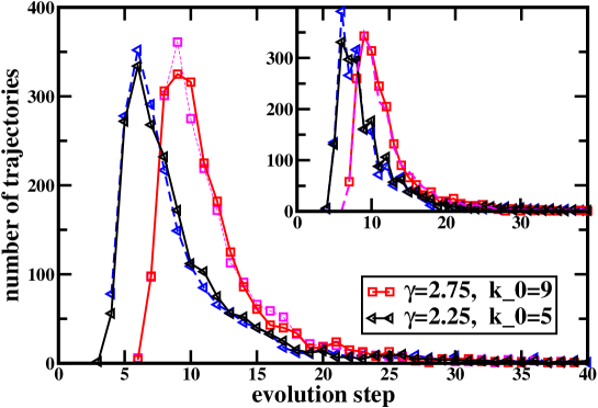
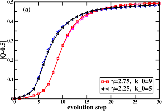
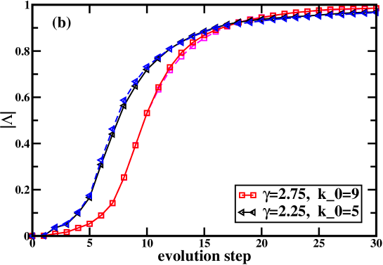
Since $Q=1/2$ represents an unstable fixed point for the time evolution of the $nn$–spin up probability $Q(t)$, a natural question to ask is the typical time needed for the system to escape from $Q=1/2$. Figure 1 displays the histogram of the decay times $t_{d}$ needed for the system to evolve from $Q(t_{0})=1/2$ at time $t_{0}$ to $|Q(t_{0}+t_{d})-1/2|>1/4$ at time $t_{0}+t_{d}$. For the four scale-free random networks with mean vertex degree $\langle k\rangle\simeq 20$, we find that the typical decay time is positively correlated with the scaling exponent $\gamma$. The most probable decay time, for example, is $t_{d,mp}=6$ for $\gamma=2.25$ but $t_{d,mp}=9$ for $\gamma=2.75$. Figure 2 shows the mean value of $Q(t)$ and $\Lambda(t)$ as a function of time $t$ for the same four different random networks. As the scaling exponent $\gamma$ becomes smaller, the system approaches the completely ordered patterns more quickly.

Figure 2: Time evolution of (A) the $nn$–spin up probability $Q(t)$ and (B) the average spin value $\Lambda(t)$ for parallel local majority-rule dynamics on an uncorrelated random multi-network of size $N=2^{18}$ and mean vertex degree $\langle k\rangle\simeq 20$. Time is measured in units of iteration steps. The four sets of data correspond to the same four scale-free random networks as in Fig. 1.

To understand this difference in decay times, we now estimate the mean decay time according to our mean-field theory. For this purpose, we define the order parameter

$$y\equiv Q-1/2\ .$$ (28)

The order parameter $y$ vanishes for all the boundary patterns satisfying Eq. (27). In the vicinity of $y=0$, the evolution of $y$ is governed by the following linearized evolution equation

$$y(t+1)=\Psi^{\prime}(1/2)y(t)\ ,$$ (29)

where $\Psi^{\prime}(1/2)\equiv{\rm d}\Psi/{\rm d}Q|_{Q=1/2}$ is expressed as

$$\Psi^{\prime}(1/2) = \sum\limits_{k}\sum\limits_{m>k/2}^{k}{kP(k)\over\langle k\rangle}B(k,m)2^{1-k}(2m-k)$$ (30)

$$= \sum\limits_{m=0}^{\infty}{(2m+1)^{2}P(2m+1)\over\langle k\rangle 2^{2m}}B(2m,m)+\sum\limits_{m=1}^{\infty}{(2m)^{2}P(2m)\over\langle k\rangle 2^{2m}}B(2m,m)\ .$$

The binomial coefficient in Eq. (30) can be estimated by Stirling’s formula which leads to

$$B(2m,m)={(2m)!\over m!m!}\approx{2^{2m}\over\sqrt{\pi}}m^{-1/2}\ .$$ (31)

If this relation is inserted into Eq. (30), we obtain

$$\Psi^{\prime}(1/2)\approx{\sqrt{2/\pi}\over\langle k\rangle}\sum\limits_{k}k^{{3\over 2}}P(k)\ .$$ (32)

In the limit of large network size $N$, Eq. (32) is well approximated by

$$\Psi^{\prime}(1/2)\approx\bigl{(}{2k_{0}\over\pi}\bigr{)}^{1/2}{(\gamma-2)\over\bigl{(}{5\over 2}-\gamma\bigr{)}}{(k_{\rm max}/k_{0})^{(5-2\gamma)/2}-1\over 1-(k_{0}/k_{\rm max})^{\gamma-2}}\ .$$ (33)

In the limiting case of $\gamma=5/2$ and $\gamma=2$, the expressions for $\Psi^{\prime}(1/2)$ is, respectively,

$$\Psi^{\prime}(1/2) \approx \bigl{(}{k_{0}\over 2\pi}\bigr{)}^{1/2}{\ln(k_{\rm max}/k_{0})\over 1-(k_{0}/k_{\rm max})^{1/2}}\hskip 14.22636pt{\rm for}\;\;\;\;\gamma=5/2$$ (34)

$$\Psi^{\prime}(1/2) \approx 2\bigl{(}{2k_{0}\over\pi}\bigr{)}^{1/2}{(k_{\rm max}/k_{0})^{1/2}-1\over\ln(k_{\rm max}/k_{0})}\hskip 14.22636pt{\rm for}\;\;\;\;\gamma=2\ .$$ (35)

Finally, using the relation that $k_{\rm max}=k_{0}N^{1/(\gamma-1)}$ as given by Eq. (2) for sufficiently large network size $N$, we obtain the following asymptotic behavior for $\Psi^{\prime}(1/2)$

$$\Psi^{\prime}(1/2) \approx 2\sqrt{2k_{0}/\pi}N^{1/2}/\ln(N)\hskip 14.22636pt{\rm for}\;\;\;\;\gamma=2\ ,$$ (36)

$$\approx \sqrt{2k_{0}/\pi}{\gamma-2\over{5\over 2}-\gamma}N^{{5-2\gamma\over 2(\gamma-1)}}\hskip 14.22636pt{\rm for}\;\;\;\;2<\gamma<5/2\ ,$$

$$\approx {1\over 3}\sqrt{2k_{0}/\pi}\ln(N)\hskip 14.22636pt{\rm for}\;\;\;\;\gamma=5/2\ ,$$

$$\approx \sqrt{2k_{0}/\pi}{\gamma-2\over\gamma-{5\over 2}}\hskip 14.22636pt{\rm for}\;\;\;\;\gamma>5/2\ .$$

From Eq. (36) we know that $\Psi^{\prime}(1/2)$ is independent of network size $N$ for $\gamma>5/2$ while it increases with $N$ for $\gamma\leq 5/2$. Since the slope $\Psi^{\prime}(1/2)$ determines the evolution of $y(t)$ for small $y$, we expect to see a qualitative change at $\gamma=5/2$.

Iterating the linear evolution equation (29) $n$ times from an initial time $t_{0}$ up to a final time $t_{1}$, one obtains the time difference

$$\Delta t_{01}\equiv t_{1}-t_{0}\approx{\ln|y(t_{1})|-\ln|y(t_{0})|\over\ln\Psi^{\prime}(1/2)}$$ (37)

in the limit of small $y(t_{0})$.

Now consider an initial state of the network at time $t=t_{0}$ that corresponds to a strongly disordered pattern with order parameter $y(t_{0})=\pm 1/(2M)=\pm 1/\langle k\rangle N$ where $M$ denotes the total number of edges with $2M=\sum_{i}k_{i}$. We characterize the decay of this strongly disordered patterns by the decay time $t_{d}$, which is the time it takes to reach a pattern with an order parameter $y_{*}$ that satisfies $|y_{*}|\geq 1/4$. Using Eq. (37) with $t_{1}\equiv t_{d}$ as well as the asymptotic expressions (36) for $\Psi^{\prime}(1/2)$, the functional dependence of the decay time $t_{d}$ on the network size $N$ is found to be Zhou and Lipowsky (2005)

$$\begin{array}[]{lll@{\qquad{\rm for}\quad}l}t_{d}&\sim&\ln(N)&\gamma>5/2\\[10.76385pt] &\sim&\ln(N)/\ln\ln(N)&\gamma=5/2\\[10.76385pt] &\sim&2(\gamma-1)/(5-2\gamma)&2<\gamma<5/2\\ \end{array}$$

in the limit of large $N$. Equation (III.1) predicts that, for random scale-free networks with $2<\gamma<5/2$, strongly disordered patterns always escape from the unstable fixed point after a finite number of iteration steps even in the limit of large $N$. In contrast, for networks with $\gamma>5/2$, the escape time diverges as $\ln(N)$. This latter behavior also applies to Poisson networks and other types of networks with single-peaked vertex degree distributions. The $\ln(N)$ scaling in response times was predicted for opinion spreading on social networks Krapivsky and Redner (2003); Aldana and Larralde (2004); Sood and Redner (2005), it was also observed in simulations of information spreading on small-world networks Zhu et al. (2004).

We will check these mean-field predictions in Sec. IV and Sec. V by extensive computer simulations.

III.2 Random sequential or asynchronous updating

Next, we apply our mean-field analysis to random sequential or asynchronous updating. In this case, we randomly choose single spins. Each single spin update corresponds to the time step $\Delta t=1/N$ which becomes small for large $N$. It is now useful to consider the quantity $\Delta n(k,t)$ which represents the change in the number of up spins on all $k$–vertices during such a single spin update. The average value of this quanitity is given by

$$\langle\Delta n(k,t)\rangle=P(k)\,[1-q_{k}(t)]\,q_{k}(t+\Delta t)-P(k)\,q_{k}(t)\,[1-q_{k}(t+\Delta t)]\,.$$ (38)

The total number of up spins on all $k$–vertices then changes according to

$$NP(k)q_{k}(t+\Delta t)=NP(k)q_{k}(t)+\langle\Delta n(k,t)\rangle\,.$$ (39)

Using the expansion $q_{k}(t+\Delta t)\approx q_{k}(t)+\Delta t\,{\rm d}q_{k}(t)/{\rm d}t$ for large $N$ or small $\Delta t=1/N$ on the left hand side and inserting the expression (38) for $\Delta n(k,t)\rangle$ on the right hand side, we obtain

$$\frac{{\rm d}q_{k}(t)}{{\rm d}t}=-q_{k}(t)+q_{k}(t+\Delta t)\,.$$ (40)

In addition, the up spin probability $q_{k}(t+\Delta t)$ is still given by (24) which leads to the continous-time evolution equations

$${{\rm d}q_{k}(t)\over{\rm d}t}=-q_{k}(t)+{\sum_{m}}^{\prime}(1-\frac{1}{2}\delta_{m,k/2})\,B(k,m)\,[Q(t)]^{m}\bigl{[}1-Q(t)\bigr{]}^{k-m}$$ (41)

for the spin up probabilities $q_{k}(t)$ and

$${{\rm d}Q(t)\over{\rm d}t}=-Q(t)+\Psi\bigl{(}Q(t)\bigr{)}$$ (42)

for the $nn$–spin up probability $Q(t)$ where $\Psi(Q)$ is still given by (26). Equation (42) has again three fixed points, two stable ones at $Q=0$ and $Q=1$ as well as an unstable one at $Q=1/2$.

As in the scheme with parallel updating, we define a new order parameter $y=Q-1/2$, compare (28). For an initial value $y(t_{0})\sim 1/N$ that represents a strongly disordered initial pattern, the order parameter $y(t)$ behaves as

$$y(t_{1})\approx y(t_{0})e^{(\Psi^{\prime}(1/2)-1)(t_{1}-t_{0})}$$ (43)

which implies the time difference

$$\Delta t_{01}\equiv t_{1}-t_{0}\approx{\ln y(t_{1})-\ln y(t_{0})\over\Psi^{\prime}(1/2)-1}\ .$$ (44)

We again characterize the decay of this strongly disordered patterns by the decay time $t_{1}=t_{d}$, which is the time it takes to reach a pattern with an order parameter $y_{*}$ that satisfies $|y_{*}|\geq 1/4$. Using the initial value $y(t_{0})\sim 1/N$, we now obtain from (44) that the typical decay time $t_{d}$ scales as

$$\begin{array}[]{lll@{\qquad{\rm for}\quad}l}t_{d}&\sim&\ln(N)&\gamma>5/2\\[10.76385pt] &\sim&N^{0}&\gamma=5/2\\[10.76385pt] &\sim&N^{0}&2<\gamma<5/2\\ \end{array}$$

in the limit of large network size $N$. Equation (III.2) is qualitatively very similar to the scaling relation (III.1) for the parallel updating scheme. A transition in dynamic behavior is therefore also predicted for random sequential local majority-rule dynamics. For uncorrelated scale-free random networks with $\gamma>5/2$, Eq. (III.2) again predicts a logarithmic scaling of the typical decay time $t_{d}$ with network size $N$. When the scaling exponent $\gamma<5/2$, on the other hand, the typical decay time is independent of $N$. The case $\gamma=5/2$ is special since the mean-field analysis predicts that $t_{d}$ is independent of $N$ for random sequential updating but grows logarithmically with $N$ for parallel updating.

IV Simulation results for random multi-networks

As a complementary approach to our mean-field analysis in Sec. III, in this and the following section, we perform local majority-rule dynamics on individual random scale-free networks. In this section, the substrate networks are generated by rule A of Sec. II.2. These multi-networks are completely random and uncorrelated, and typically contain both self-connections and multiple edges.

After a network is constructed with given parameters $N$, $\gamma$, and $k_{0}$, a random initial spin pattern $\{\sigma_{i}(0)\}$ is assigned to vertices of the network. The system then evolves according to Eq. (9) for parallel updating and according to Eq. (10) for random sequential updating. Each resulting trajectory is monitored and the values of $\Lambda(t)$ and $Q(t)$ as defined in Eq. (13) and Eq. (18), respectively, are recorded at each time point $t$. The initial spin patterns are chosen such that the average spin value $\Lambda$ and the $nn$–spin up probability $Q$ have the initial values

$$\Lambda(0)\equiv 0\quad{\rm and}\quad Q(0)\equiv{1\over 2}\ ,$$ (45)

i.e., these patterns are disordered both with respect to the average spin value and with respect to the $nn$–spin up probability. We track each trajectory until the two conditions $|\Lambda(t)|>1/2$ and $|Q(t)-1/2|>1/4$ are both satisfied. For each random network, $2,000$ such trajectories are simulated and analyzed in order to estimate the median decay time.

Figure 3: Median decay time $t_{d,m}$ as a function of network size $N$ for random multi-networks and parallel or synchronous updating. Each data point is obtained by performing simulations on $100$ multi-networks. (a) Median decay time needed to reach a partially ordered pattern characterized by $|Q(t)-1/2>1/4|$ for the first time; and (b) Median decay time needed to reach a partially ordered pattern with $|\Lambda(t)>1/2|$ for the first time.

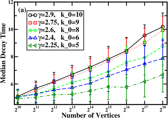
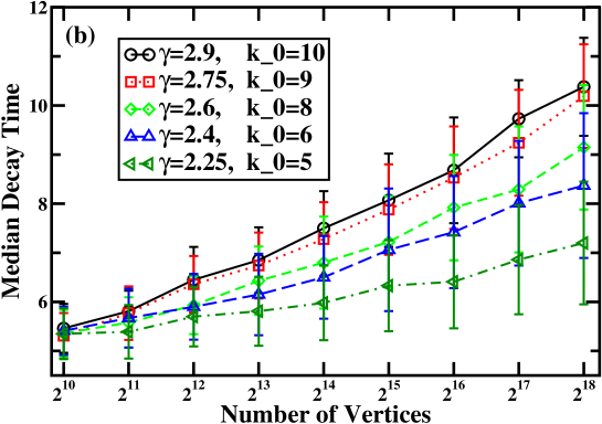
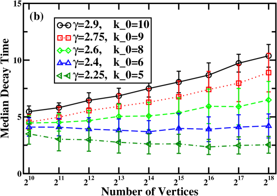
In our previous study Zhou and Lipowsky (2005), we used parallel or synchronous updating in order to generate the time evolution of the activity patterns. In the present study, we use both parallel updating and random sequential or asynchronous updating and check the robustness of our qualitative conclusions in Ref. Zhou and Lipowsky (2005). For parallel updating, our simulational results are summarized in Fig. 3, for random sequential in Fig. 4. In these figures, we plot the median decay time, $t_{d,m}$, as a function of the network size or vertex number $N$. By definition, the median decay time $t_{d,m}$ splits the decay time histogram up into two parts of equal size, i.e., the probability to observe a decay time $t_{d}$ with $t_{d}<t_{d,m}$ is equal to the probability to observe one with $t_{d}>t_{d,m}$. In Fig. 3(a) and Fig. 4(a), we display the median decay time needed for the system to reach a pattern characterized by $|Q(t)-Q(0)|\geq 1/4$ from an initial strongly disordered pattern, which satisfies Eq. (45). Likewise, in Fig. 3(b) and Fig. 4(b), we show the median decay time for the system to attain a pattern characterized by $|\Lambda(t)|\geq 1/2$ starting again from an initially disordered pattern satisfying Eq. (45).

Figure 4: Median decay time $t_{d,m}$ as a function of network size $N$ for random multi-networks and random sequential or asynchronous updating. Each data point is obtained by performing simulations on the same set of $100$ random multi-networks as in Fig. 3. (a) Median decay time needed for $|Q(t)-1/2|$ to exceed $1/4$ for the first time. (b) Median decay time needed for $|\Lambda(t)|$ to exceed $1/2$ for the first time.

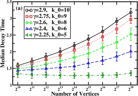
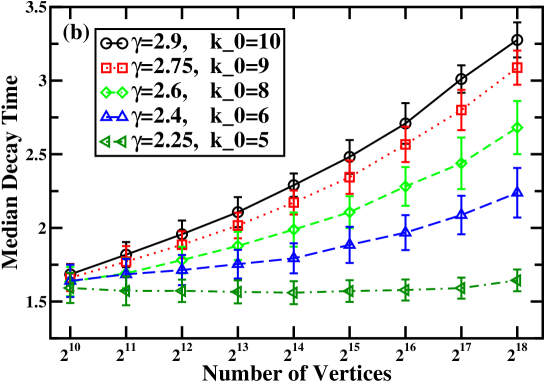
The data for parallel updating of multi-networks as shown in Fig. 3 do not exhibit a clear distinction between networks with $\gamma>5/2$ and those with $\gamma<5/2$. In contrast, the data for random sequential updating of multi-networks as shown in Fig. 4 exhibit such a distinction, at least for $\gamma=2.25$ and $\gamma=2.6$. For scaling exponent $\gamma\geq 2.6$, the median decay times $t_{d,m}$ increases with network size $N$ according to $t_{d,m}\sim(\ln N)^{\eta}$, where the exponent $\eta$ appears to be slightly larger than $1$. Our mean field theory predicts $\eta=1$. For $\gamma=2.25$, which is smaller than but not close to $\gamma=5/2$, the median decay time $t_{d,m}$ is found to be independent of network size $N$, see Fig. 4(a) and (b), in agreement with our mean-field prediction. However, for $\gamma=2.4$, which is smaller than but close to $\gamma=5/2$, inspection of Fig. 4 indicates that the median decay time increases slowly with network size $N$. This observation disagrees with our mean field prediction.

V Simulation results for random simple-networks

The random multi-networks discussed in the previous Sec. IV contain self-connections and multiple edges between the same pair of vertices. Such connections are absent in many real networks. Thus, we will now consider the temporal evolution of activity patterns on random simple-networks without self-connections and multiple edges. As previously mentioned, such networks exhibit some vertex degree correlations.

We use rule B as described in Sec. II.2 in order to generate an ensemble of scale-free random simple-networks. Each vertex of the network is occupied by a binary variable or spin which evolves again according to local majority rule dynamics. We use both parallel and random sequential updating starting from random initial conditions as specified by Eq. (45). The degree sequences of the generated networks are the same as those used in the preceding section. Therefore, if the results of this subsection are different from those of Sec. IV, the differences must be related to the correlations in the random simple-networks. Our simulational results are summarized in Fig. 5 and Fig. 6 for parallel and random sequential updating, respectively.

Figure 5: Median decay time as a function of network size $N$ for random simple-networks and parallel or synchronous updating. Each data point is obtained by performing simulations for an ensemble of $100$ networks. Each simulation run starts from an initial spin or activity pattern characterized by relation (45). (a) Median decay time needed to reach a spin pattern for which the $nn$–spin up probability $Q(t)$ satisfies $|Q(t)-1/2|>1/4$ for the first time; and (b) Median decay time needed to reach a spin pattern for which the average spin value $\Lambda(t)$ exceeds $1/2$ for the first time.

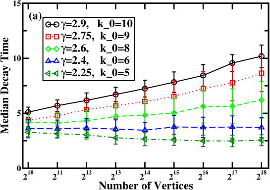
In Fig. 5(a) and Fig. 6(a), we display the median decay time $t_{d,m}$ needed for the network to reach an activity pattern that is characterized by a $nn$–spin up probability $Q(t)$ that satisfies $|Q(t)-Q(0)|\geq 1/4$ when the initial pattern is characterized by the relation (45). Likewise, in Fig. 5(b) and Fig. 6(b), we show the median decay time for the network to reach a pattern with average spin value $|\Lambda(t)|\geq 1/2$ starting again from an initial pattern which satisfies (45).

Figure 6: Median decay time as a function of vertex size $N$ for random simple-networks and random sequential or asychronous updating. Each data point is obtained by performing simulations for the same ensemble of $100$ simple-networks as in Fig. 5. (a) Median decay time needed for $|Q(t)-1/2|$ to exceed $1/4$ for the first time; and (b) Median decay time needed for $|\Lambda(t)|$ to exceed $1/2$ for the first time.

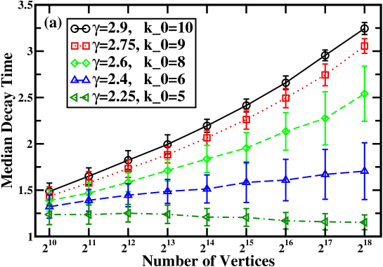
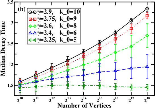
For scaling exponent $\gamma>5/2$, the median decay time $t_{d,m}$ increases with network size $N$ as $t_{d,m}\sim(\ln N)^{\eta}$ with a growth exponent $\eta$ that again appears to be slightly larger than the mean field value $\eta=1$. The same behavior was observed in the preceding section for random multi-networks. For $\gamma=2.25$, which is smaller than but not close to $\gamma=5/2$, the median decay times are essentially independent of the network size $N$. The latter behavior was also found for random sequential updating of multi-networks. For $\gamma=2.4$, i.e., smaller than but close to $\gamma=5/2$, on the other hand, both Fig. 5 and Fig. 6 demonstrate that the median decay time first increases slowly and then saturates for increasing network size $N$. In other words, the function $t_{d,m}=t_{d,m}(\ln N)$ is now convex downwards. This situation is remarkably different from what was found in random multi-networks, see Fig. 3 and Fig. 4, for which the function $t_{d,m}=t_{d,m}(\ln N)$ is convex upwards over the whole range of accessible $N$–values. Therefore, for random simple-networks, we conclude that the median decay time $t_{d,m}$ becomes independent of network size $N$ in the limit of large $N$ if the scaling exponent $\gamma$ of the scale-free degree distribution satisfies $\gamma<5/2$ as predicted by mean field theory.

VI Effective scaling exponent for multi-networks

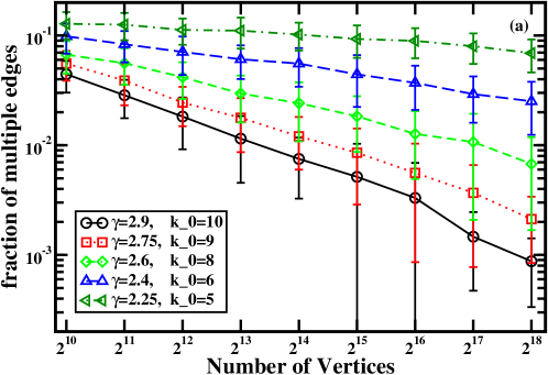
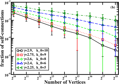
Multi-network typically contain self-connections and multiple edges. As shown in Fig. 7(a), the fraction of edges that represent multiple edges is found to vary between about $10^{-1}$ and $10^{-3}$ depending on the number $N$ of vertices and the scaling exponent $\gamma$ of the scale-free degree distribution. Furthermore, the fraction of edges that represent self-connections varies between $10^{-2}$ and $10^{-5}$, see Fig. 7(b). Both fractions decrease with increasing network size $N$ and increase with decreasing scaling exponent $\gamma$. This behavior can be understood from the following considerations.

In a random multi-network, the probability that an edge is a self-connection of vertex $i$ is equal to $\bigl{(}k_{i}/\sum_{j}k_{j}\bigr{)}^{2}=k_{i}^{2}/(4M^{2})$, where $k_{i}$ is the degree of vertex $i$ and $M$ is the total number of edges as before. The average number of self-connections of a certain vertex $i$ with degree $k_{i}$ is then given by $k_{i}^{2}/4M$. Therefore, the total number of self-connections is estimated to be

$$M_{\rm self} = \sum\limits_{i=1}^{N}{k_{i}^{2}\over 4M}=\sum\limits_{k}NP(k){k^{2}\over 4M}$$ (46)

$$\approx {k_{0}^{2}(\gamma-1)\over 2\langle k\rangle(3-\gamma)}{N^{(3-\gamma)/(\gamma-1)}-1\over 1-1/N}$$ (47)

for a scale-free network with scaling exponent $\gamma$. This relation shows that, for $\gamma\geq 3$, the total number of self-connetions is of order unity. In contrast, for scale-free networks with $2<\gamma<3$, the total number $M_{\rm self}$ of self-connections scales with network size $N$ as $M_{\rm self}\sim N^{(3-\gamma)/(\gamma-1)}$ for large $N$. Therefore, the fraction of self-connections decays as $M_{\rm self}/M\sim N^{(4-2\gamma)/(\gamma-1)}$ with increasing network size $N$.

Likewise, in a random multi-network, the probability that an edge is formed between a certain vertex $i$ with degree $k_{i}$ and another vertex $j$ with degree $k_{j}$ is given by

$$2{k_{i}\over\sum_{l}k_{l}}{k_{j}\over\sum_{l}k_{l}}={k_{i}k_{j}\over 2M^{2}}\ .$$ (48)

Using this probabilility, one may derive an approximate expression for the total number $M_{mult}$ of multiple edges. The formula is a little bit more complex than Eq. (47) so we do not write down the explicit formula here. The average number of multiple edges is also found to be of order unity for $\gamma\geq 3$ and to increase with network size $N$ as a power-law for $2<\gamma<3$. This is consistent with the data shown in Fig. 7(a).

Figure 7: Fraction of (a) multiple edges and (b) self-connections in a random scale-free multi-network. Each data point is an average over the same ensemble of $100$ random networks as used in the simulations of the preceding sections.

Furthermore, we find that the removal of all self-connections and multiple edges from a scale-free multi-network leads to a simple-network that is again scale free but with the modified vertex degree distribution

$$P_{\rm eff}(k)\sim k^{-\gamma_{\rm eff}}\quad{\rm with}\quad\gamma_{\rm eff}=\gamma_{\rm eff}(\gamma,N)\,.$$ (49)

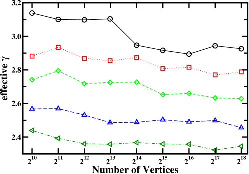
In Eq. (49), $k$ is the effective degree of a vertex, i.e., the number of connections of the vertex after all its self-connections are removed and all its multiple edges are reduced to a single edge. The scaling exponent $\gamma_{\rm eff}$ can be obtained by calculating the cumulative distribution function of the effective degree $k$ Newman (2005). The functional dependence of the effective scaling exponent $\gamma_{\rm eff}$ on the scaling exponent $\gamma$ of the original multi-network and on the network size $N$ is displayed in Fig. 8. Inspection of this figure shows that the effective scaling exponent satisfies $\gamma_{\rm eff}\geq\gamma$ and decreases towards $\gamma$ with increasing network size $N$. For $\gamma=2.9,2.75$, and 2.6, the data strongly indicate that the effective exponent $\gamma_{\rm eff}$ becomes asymptotically equal to $\gamma$ for large $N$. We expect that the same behavior applies to the multi-networks with $\gamma<5/2$ but this remains to be shown.

Now, let us focus on the case $\gamma=2.4$ for which we found some qualitative differences between multi- and simple-networks. As shown in Fig. 8, the effective scaling exponent is found to satisfy $\gamma_{\rm eff}\mathrel{\mathchoice{\vbox{\offinterlineskip\halign{\hfil$\displaystyle#$\hfil\cr>\cr\sim\cr}}}{\vbox{\offinterlineskip\halign{\hfil$\textstyle#$\hfil\cr>\cr\sim\cr}}}{\vbox{\offinterlineskip\halign{\hfil$\scriptstyle#$\hfil\cr>\cr\sim\cr}}}{\vbox{\offinterlineskip\halign{\hfil$\scriptscriptstyle#$\hfil\cr>\cr\sim\cr}}}}2.5$ up to $N=2^{17}$ for multi-networks with $\gamma=2.4$. Thus, these multi-networks lead to simple-networks with $\gamma_{\rm eff}\geq 5/2$ for almost all values of $N$ that are accessible to the simulations. In this way, we obtain a rather intuitive explanation for our difficulty to confirm the mean field predictions for multi-networks with $\gamma=2.4$.

Figure 8: Effective scaling exponent $\gamma_{\rm eff}$ for random simple-networks that have been obtained by removal of all multiple edges and self-connections from an ensemble of random multi-networks. Each data point is obtained by merging all the $100$ vertex degree sequences corresponding to the $100$ multi-networks used in the simulation. The degree distributions of these multi-networks are characterized by the parameter values $\gamma=2.25$, $k_{0}=5$ (triangles left), $\gamma=2.4$, $k_{0}=6$ (triangles up), $\gamma=2.6$, $k_{0}=8$ (diamonds), $\gamma=2.75$, $k_{0}=9$ (squares), and $\gamma=2.9$, $k_{0}=10$ (circles).

As far as the network’s topology is concerned, both self-connections and multiple edges can be regarded as redundant. However, these self-connections and multiple edges have very significant effects for the dynamics of activity patterns of these networks. Let us consider the following simple example. Suppose there are two high-degree vertices $i$ and $j$ with initial spin state $\sigma_{i}=1$ and $\sigma_{j}=-1$. Each of these two vertices is taken to have many self-connections, and there are many edges between them. The self-connections tend to stabilize the current spin state of each vertex, while the edges between $i$ and $j$ tend to align the two spins. The frustration caused by the competition of these two effects can lead to an increase in the relaxation time. More generally, in a scale-free multiple network with $\gamma<3$, there exists a densly connected core of high-degree vertices. Each vertex of this core has many self-connections (which tend to stabilize its current spin state) and is connected by multiple edges to many vertices in this core (which tend to align the spins on neighboring vertices). Starting from a random initial spin configuration, spin state frustrations may easily build up within such a core. Such frustrations can be ‘annealed’ by external influences as provided, e.g., by the interactions with vertices outside the core, but for scale-free multi-networks with $\gamma\sim 5/2$, this annealing process may take a relatively long time, since the fraction of ‘redundant’ edges is high and the effective scaling exponent is larger than $5/2$.

In our simulation, we have studied only the dynamic properties of random scale-free networks. In general, the vertex degrees of neighboring vertices may be correlated. In the case of simple networks, these correlations are caused by prohibition of self-connections and multiple edges Maslov and Sneppen (2002); Maslov et al. (2002); Boguñá et al. (2004); Catanzaro et al. (2005); in the case of multiple networks, these correlations exist between the effective vertex degrees of neighboring vertices. Such correlations of vertex degrees may also have some influence on the majority-rule dynamics. In order to study the influence of vertex degree correlations on the dynamic network processes in a quantitative manner, one may generate ensembles of random networks with specified vertex degree and specified vertex correlation patterns (see, e.g., Maslov et al. (2002)). In fact, the co-evolution of correlations in the network structure and network dynamics represents a rather interesting topic for future studies.

VII Conclusion and discussion

We have studied the time evolution of activity patterns on scale-free random networks which are characterized by the degree distribution $P(k)\sim 1/k^{\gamma}$ for $k_{0}<k<k_{max}$. We constructed two different ensembles of such networks as explained in Section II.2: (A) multi-networks with self-connections and multiple edges as generated by the configuration method and (B) simple-networks without any self-connections and multiple edges as generated by a combination of the configuration method and an edge switching or reshuffling algorithm. We focussed on networks with minimal vertex degree $k_{0}\geq 5$ for which all network graphs were found to consist of only a single component.

On each vertex of these networks, we place a binary variable or Ising-like spin $\sigma_{i}=\pm 1$. For a given network with $N$ vertices, the activity pattern at time $t$ is described by the spin configuration $\{\sigma(t)\}\equiv\{\sigma_{1}(t),\sigma_{2}(t),\dots,\sigma_{N}(t)\}$. The time evolution of this pattern is govened by local majority dynamics, which represents a Markov process in pattern space and is equivalent to Glauber dynamics at zero temperature. We used two different updating schemes as explained in Section II.3: (i) parallel or synchronous updating as defined by (9) and (ii) random sequential or asynchronous updating as in (10).

We focussed on the relaxation or decay of initial activity patterns that are strongly disordered both with respect to the average spin value $\Lambda=\langle\sigma\rangle$ as given by (13) and with respect to the $nn$–spin up probability $Q$ as defined in (15) (where $nn$ stands for ‘nearest neighbor’). Indeed, these initial patterns are chosen to satisfy $\Lambda=0$ and $Q=1/2$ as in (45). The relaxation process is measured by the decay time $t_{d}$ it takes to reach a pattern with $|\Lambda|\geq 1/2$ and/or $|Q-1/2|\geq 1/4$. This decay time is governed by a single peak distribution from which we determined the median decay time $t_{d,m}$.

The mean field theory described in Section III predicts that the $N$–dependence of the decay time is different for scaling exponents $\gamma<5/2$ and $\gamma>5/2$. For $\gamma<5/2$, the typical decay time remains finite even in the limit of large network size $N$. In contrast, this time scale increases as $\ln N$ with increasing $N$ for $\gamma>5/2$. In order to check these mean field predictions, we have performed four types of numerical simulations corresponding to parallel and random sequential updating of multi- and simple-networks.

The simulation data for parallel updating of multi-networks are shown in Fig. 3. In this case, the median decay time is found to increase with network size $N$ up to $N=2^{18}$ for all values of $\gamma$. Random sequential updating of the same ensemble of multi-networks leads to the data shown in Fig. 4. Inspection of this latter figure shows that the median decay time is now essentially independent of $N$ for $\gamma=2.25$ as predicted by mean field theory. However, for $\gamma=2.4$, this time scale still seems to increase with $N$ in contrast to the mean field predictions. This apparent increase can be understood if one defines an effective scaling exponent $\gamma_{\rm eff}$ for multi-networks as discussed in Section VI. As shown in Fig. 8, this effective scaling exponent decreases monotonically with increasing network size $N$ and satisfies $\gamma_{\rm eff}\geq\gamma$. In particular, for multi-networks with $\gamma=2.4$, we find $\gamma_{\rm eff}\mathrel{\mathchoice{\vbox{\offinterlineskip\halign{\hfil$\displaystyle#$\hfil\cr>\cr\sim\cr}}}{\vbox{\offinterlineskip\halign{\hfil$\textstyle#$\hfil\cr>\cr\sim\cr}}}{\vbox{\offinterlineskip\halign{\hfil$\scriptstyle#$\hfil\cr>\cr\sim\cr}}}{\vbox{\offinterlineskip\halign{\hfil$\scriptscriptstyle#$\hfil\cr>\cr\sim\cr}}}}5/2$ up to $N=2^{17}$.

The simulation data for parallel and random sequential updating of simple-networks are shown in Fig. 5 and Fig. 6, respectively. In this case, both updating schemes are in complete agreement with the mean field predictions. Thus, we conclude that mean field theory is valid for the ensemble of random simple-networks but is more difficult to confirm for the ensemble of random multi-networks because of strong finite size effects as described by the $N$–dependent value of the effective scaling exponent $\gamma_{\rm eff}$.

In the present article, we have analyzed the time evolution of strongly disordered patterns at $t=0$ into partially ordered patterns characterized by $|\Lambda|>1/2$ and/or $|Q-1/2|>1/4$ at $t=t_{d}$. These partially ordered patterns further evolve towards completely ordered patterns. If the network has $\kappa$ components, one has $2^{\kappa}$ such ordered patterns. However, there is always a small but non-zero probability that the local majority rule dynamics does not achieve complete order Castellano and Pastor-Satorras (2006). One major reason for this failure is the existence of small network components with certain ‘balanced’ shapes that lead to domain boundaries and blinkers Svenson (2002); Häggström (2002). The probability to find such components is expected to decrease with increasing mean vertex degree $\langle k\rangle$ and increasing minimal vertex degree $k_{0}$.

Both for $d$-dimensional regular lattices Spirin et al. (2001) and for tree-like networks Mélin et al. (1996), the time evolution of activity patterns typically leads to metastable states with many domain boundaries and blinkers. In contrast, we did not find such a behavior for random scale-free networks with $k_{0}\geq 2$ as studied here. Indeed, our simulations show that most of the spins are already aligned after about 30 time steps, see Fig. 2.

Our mean field analysis can also be applied to more complicated dynamical models as we have previously discussed in Zhou and Lipowsky (2005). One such extension is provided by finite-connectivity Hopfield models Hopfield (1982) on scale-free random networks. In this case, our mean field theory predicts the storage capacity to grow as $N^{\alpha}$ with network size $N$ where the growth exponent $\alpha$ satisfies $1>\alpha>0$ provided $2<\gamma<5/2$. According to recent experimental studies Chialvo (2004); Eguiluz et al. (2005), the functional networks of the human brain are scale-free with a scaling exponent $\gamma\simeq 2.1$. In the latter case, our mean field theory leads to a storage capacity that grows as $N^{\alpha}$ with $\alpha\simeq 0.73$, i.e., almost as fast as for the original Hopfield models on complete graphs.

Likewise, we have extended our mean field theory to scale-free networks for which each vertex $i$ contains a Potts-like variable $\sigma_{i}$ that can attain $q\geq 3$ values. These dynamic systems exhibit $q$ ordered patterns (in each network component) and may evolve towards any of those patterns when they start from a strongly disordered one. For these Potts-like systems, we find the same distinction between the relaxation behavior for scale-free networks with $\gamma<5/2$ and $\gamma>5/2$ as in the case of the Ising-like systems studied here. We also considered some hybrid dynamics constructed from local majority dynamics and random Boolean dynamics: each spin variable $\sigma_{i}$ is updated with probability ${\cal P}$ according to local majority rule dynamics and with probability $1-{\cal P}$ according to random Boolean dynamics as in the Kauffman models Kauffman (1969); Derrida and Pomeau (1986). As long as ${\cal P}>0$, the relaxation behavior of this more general class of models shows the same qualitative change at $\gamma=5/2$. Finally, we have extended our mean field theory to binary or Ising-like variables on directed networks, see Zhou and Lipowsky (2005). The elucidation of these mean field results by appropriate simulation studies is highly desirable and remains to be done.

VIII Appendix: Upper cut-off for vertex degree

In this appendix, we explain the dependence of the maximal degree $k_{\rm max}^{(2)}$ on $N$ in more detail. In Ref. Cohen et al. (2000), the scaling $k_{\rm max}^{(2)}\sim N^{{1\over\gamma-1}}$ was obtained from the requirement that the average number of vertices with degree $k\geq k_{\max}^{(2)}$ should be of order one, that is

$$N{\sum\limits_{k=k_{\rm max}^{(2)}}^{\infty}k^{-\gamma}\over\sum\limits_{k=k_{0}}^{\infty}k^{-\gamma}}\simeq 1\ .$$ (50)

It is instructive to rederive the same scaling relation for $k_{\rm max}^{(2)}$ through an alternative way. To do this, we start from the scale-free degree distribution $P_{\infty}(k)$ which has the same form as that of $P(k)$ in Eq. (3) but with $k_{\max}=\infty$. The distribution $P_{\infty}(k)$ is used to generate $N$ random numbers $x_{i}$ with $i=1,2,\ldots,N$ and $x_{i}\geq k_{0}$ which correspond to the vertex degrees of the $N$ vertices. Since the normalization factor ${\cal A}$ as given by Eq. (4) behaves as ${\cal A}\approx k_{0}^{1-\gamma}/(\gamma-1)$ for large $k_{\rm max}$, the random variables $x_{i}$ are generated according to the probability density

$$P_{\infty}(x)=(\gamma-1)k_{0}^{\gamma-1}x^{-\gamma}\ .$$ (51)

The maximal value $x_{\rm max}$ of the $N$ random numbers $x_{i}$ is then governed by the probability density

$$\rho(x_{\rm max})=N(\gamma-1)k_{0}^{\gamma-1}x_{\rm max}^{-\gamma}\Bigl{(}1-\bigl{(}{k_{0}\over x_{\rm max}}\bigr{)}^{\gamma-1}\Bigr{)}^{N-1}\ .$$ (52)

It follows from this latter probability density, which is normalized as well, that $x_{\rm max}$ has the average value

$$\langle x_{\rm max}\rangle=Nk_{0}B\bigl{(}{\gamma-2\over\gamma-1},N\bigr{)}\ ,$$ (53)

where $B(z,N)$ is the standard beta function Abramowitz and Stegun (1972). In the limit of large network size $N$, one has $B(z,N)\approx\Gamma(z)\exp(z)N^{-z}$, which implies

$$\langle x_{\rm max}\rangle\approx k_{0}N^{1/(\gamma-1)}\ ,$$ (54)

i.e., the same $k_{0}$ and $N$ dependence as for $k_{\rm max}^{(2)}$. The same dependencies are also obtained for the most probable value of $x_{\rm max}$ which corresponds to the maximum of the distribution $\rho(x_{\rm max})$ and is given by

$$x_{\rm max}^{(mp)}=k_{0}\bigl{(}{1\over\gamma}+{\gamma-1\over\gamma}N\bigr{)}^{{1\over\gamma-1}}\ .$$ (55)

Using the probability density $\rho(x_{\rm max})$ as given by (58), we obtain for the second moment of $x_{\rm max}$ the expression

$$\langle x_{\rm max}^{2}\rangle=Nk_{0}^{2}B({\gamma-3\over\gamma-1},N)$$ (56)

For $\gamma<3$, $\langle x_{\rm max}^{2}\rangle$ is infinite since one of the arguments of the beta function in Eq. (56) is negative. Thus, the fluctuations in $x_{\rm max}$ are unbounded unless we use the natural upper cut-off $k_{\rm max}^{(1)}=N-1$.

References

- Albert and Barabási (2002) R. Albert and A.-L. Barabási, Rev. Mod. Phys. 74, 47 (2002).
- Dorogovtsev and Mendes (2002) S. N. Dorogovtsev and J. F. F. Mendes, Adv. Phys. 51, 1079 (2002).
- Newman (2003) M. E. J. Newman, SIAM Rev. 45, 167 (2003).
- Barabási and Albert (1999) A.-L. Barabási and R. Albert, Science 286, 509 (1999).
- Valverde et al. (2002) S. Valverde, R. Ferrer Cancho, and R. V. Solé, Europhys. Lett. 60, 512 (2002).
- Ferrer i Cancho and Solé (2003) R. Ferrer i Cancho and R. V. Solé, in Lecture Notes in Physics 625: Statistical Mechanics of Complex Networks, edited by R. Pastor-Satorras, M. Rubi, and A. Diaz-Guilera (Springer, Berlin, 2003), chap. 6, pp. 114–126.
- Variano et al. (2004) E. A. Variano, J. H. McCoy, and H. Lipson, Phys. Rev. Lett. 92, 188701 (2004).
- Wang et al. (2005) W.-X. Wang, B.-H. Wang, B. Hu, G. Yan, and Q. Ou, Phys. Rev. Lett. 94, 188702 (2005).
- Zhou and Lipowsky (2005) H. Zhou and R. Lipowsky, Proc. Natl. Acad. Sci. USA 102, 10052 (2005).
- Aldana and Cluzel (2003) M. Aldana and P. Cluzel, Proc. Natl. Acad. Sci. USA 100, 8710 (2003).
- Catanzaro et al. (2005) M. Catanzaro, M. Boguñá, and R. Pastor-Satorras, Phys. Rev. E 71, 027103 (2005).
- Castellano and Pastor-Satorras (2006) C. Castellano and R. Pastor-Satorras, J. Stat. Mech., P05001 (2006).
- Cohen et al. (2000) R. Cohen, K. Erez, D. ben-Avraham, and S. Havlin, Phys. Rev. Lett. 85, 4626 (2000).
- Milo et al. (2003) R. Milo, N. Kashtan, S. Itzkovitz, M. E. J. Newman, and U. Alon, On the uniform generation of random graphs with prescribed degree sequences, e-print: cond-mat/0312028 (2003).
- Zhou (2002) H. Zhou, Phys. Rev. E 66, 016125 (2002).
- Glauber (1963) R. J. Glauber, J. Math. Phys. 4, 294 (1963).
- Bar-Yam and Epstein (2004) Y. Bar-Yam and I. R. Epstein, Proc. Natl. Acad. Sci. USA 101, 4341 (2004).
- Maslov and Sneppen (2002) S. Maslov and K. Sneppen, Science 296, 910 (2002).
- Maslov et al. (2002) S. Maslov, K. Sneppen, and A. Zaliznyak, Physica A 333, 529 (2002).
- Boguñá et al. (2004) M. Boguñá, R. Pastor-Satorras, and A. Vespignani, Eur. Phys. J. B 38, 205 (2004).
- Krapivsky and Redner (2003) P. L. Krapivsky and S. Redner, Phys. Rev. Lett. 90, 238701 (2003).
- Aldana and Larralde (2004) M. Aldana and H. Larralde, Phys. Rev. E 70, 066130 (2004).
- Sood and Redner (2005) V. Sood and S. Redner, Phys. Rev. Lett. 94, 178701 (2005).
- Zhu et al. (2004) C.-P. Zhu, S.-J. Xiong, Y.-J. Tian, N. Li, and K.-S. Jiang, Phys. Rev. Lett. 92, 218702 (2004).
- Newman (2005) M. E. J. Newman, Contemporary Phys. 46, 323 (2005).
- Svenson (2002) P. Svenson, Phys. Rev. E 64, 036122 (2002).
- Häggström (2002) O. Häggström, Physica A 310, 275 (2002).
- Spirin et al. (2001) V. Spirin, P. L. Krapivsky, and S. Redner, Phys. Rev. E 65, 016119 (2001).
- Mélin et al. (1996) R. Mélin, J. C. Anglès d’Auriac, P. Chandra, and B. Doucot, J. Phys. A: Math. Gen. 29, 5773 (1996).
- Hopfield (1982) J. J. Hopfield, Proc. Natl. Acad. Sci. USA 79, 2554 (1982).
- Chialvo (2004) D. R. Chialvo, Physica A 340, 756 (2004).
- Eguiluz et al. (2005) V. M. Eguiluz, D. R. Chialvo, G. A. Cecchi, M. Baliki, and A. V. Apkarian, Phys. Rev. Lett. 94, 018102 (2005).
- Kauffman (1969) S. A. Kauffman, J. Theo. Biol. 22, 437 (1969).
- Derrida and Pomeau (1986) B. Derrida and Y. Pomeau, Europhys. Lett. 1, 45 (1986).
- Abramowitz and Stegun (1972) M. Abramowitz and I. A. Stegun, Handbook of mathematical functions (Dover Publications, New York, 1972).