Visibility of a Bose-condensed gas released from an optical lattice at finite temperatures

Résumé

In response to a recent manuscript Diener et al. (2006) on the analysis of interference patterns produced by ultracold atoms released from an optical lattice, we point out that in the presence of a Bose-Einstein condensate the interference pattern can be strongly modified by interaction effects and the presence of a harmonic trap superimposed on the lattice potential. Our results show that the visibility of the interference pattern is significant only if a sizeable condensate fraction is present in the trap, in strong contrast to the findings of ref. Diener et al. (2006).

Introduction-

Experiments with ultracold quantum gases in optical lattices rely heavily on time-of-flight expansion to probe the spatial coherence properties of the trapped gas Greiner et al. (2002); Stöferle et al. (2004); Gerbier et al. (2005a, b). When the phase coherence length is large compared to the lattice spacing, the post-expansion density distribution reveals a striking interference pattern with the same symmetry as the reciprocal lattice. As the phase coherence length decreases, e.g. on approaching the Mott insulator transition, the visibility of this interference pattern decreases accordingly, and for very short coherence length the underlying lattice order can only be revealed through higher-order correlations Fölling et al. (2005). A recent manuscript Diener et al. (2006) has raised the question, whether even a minute condensate fraction on the order of $1/(\epsilon N^{2/3})$ ($N$ being the total particle number) should give rise to an interference pattern with visibility $\mathcal{V}$ very close to unity, $\mathcal{V}\approx 1-\epsilon$. According to the calculations in Diener et al. (2006), a system of, e.g., $N=10^{5}$ atoms should show an interference pattern with a visibility of $\mathcal{V}\approx>99\%$ for minute condensate fractions $\approx 4\%$ ($\approx 5000$ atoms). As current experiments with ultracold quantum gases do not observe this (the best visibilities that have been achieved in our group being close to 90%), the authors conclude that the current experiments must be carried out in a thermal regime with no condensate or superfluid fraction present in the trap.

In this paper we would like to point out that this reverse conclusion is an artifact of the model used in Diener et al. (2006) to describe the time-of-flight expansion. A central assumption in Ref. Diener et al. (2006) is to consider that the condensate momentum distribution is Heisenberg-limited by the size of the system prior to expansion, and that this distribution is preserved in time-of-flight. Below, we would like to explain that several effects spoil this assumption, as under realistic experimental conditions, one needs to take into account:

• (i) The inhomogeneous trapping potential for the quantum gas in the lattice,

• (ii) The mean-field broadening of the momentum peaks during time-of-flight expansion,

• (iii) The finite time-of-flight in the experiments.

Practically, these effects tend to broaden the peaks present in the interference pattern, hence diminishing its peak value. In the presence of a significant non-condensed fraction, this will also lower the visibility. In cases when the initial momentum width is very large, for example for a cloud close to or in the Mott insulator regime, or a thermal gas well above the critical temperature, they can usually be neglected. However, the momentum width for a condensate is conversely very narrow. Even without an optical lattice, effects (i)-(iii) have been known to play an important role in the interpretation of time-of-flight images (see, e.g. Kagan et al. (1996); Castin and Dalibard (1997); Dalfovo et al. (1999)). We point out that a number of other effects might be relevant in a given experimental situation, for instance a finite imaging resolution, or collisions during the initial expansion phase that would scatter the atoms out of the condensate. Here we do not consider these aspects further, and consider an idealized experiment limited only by the three points above. Below we outline our arguments and point out the most critical steps to arrive at the conclusions given in Diener et al. (2006). We propose a simple model to explain why the visibility of the interference pattern follows the condensate fraction in the system at least in a qualitative way. We also find that for the parameters that correspond to current experiments, the visibility of an expanding, non-condensed thermal cloud is always significantly lower than $1$, a conclusion consistent with experiments Greiner et al. (2002); Stöferle et al. (2004); Gerbier et al. (2005a, b).

Setup and Optical Lattice Potentials -

The optical lattice potential can be expressed as

$$V_{\rm OL}({\bf r})=V_{0}\left(\sin^{2}(k_{\rm L}x)+\sin^{2}(k_{\rm L}y)+\sin^{2}(k_{\rm L}z)\right).$$ (1)

Here $V_{0}$ is the lattice depth expressed in units of the single-photon recoil energy $E_{\rm R}=h^{2}/2m\lambda_{\rm L}^{2}$. Here $k_{\rm L}=2\pi/\lambda_{\rm L}$ is the laser wavevector, $\lambda_{\rm L}$ is the laser wavelength and $m$ is the atomic mass. In addition to the lattice potential, an “external” potential is present, due to the presence of a magnetic trap and also to the optical confinement provided by the Gaussian-shaped lattice beams. The external potential is nearly harmonic with trapping frequency

$$\omega_{\rm T}\approx\sqrt{\omega_{\rm m}^{2}+\frac{4(2V_{0}-\sqrt{V_{0}})}{mw^{2}}},$$ (2)

where $\omega_{\rm m}$ is the frequency of the magnetic trap, assumed isotropic, and where $w$ is the waist ($1/e^{2}$ radius) of the lattice beams, assumed identical for all axes. This formula, slightly different from the one given in Gerbier et al. (2005b), takes into account the modification of the vibrational ground state energy in each well due to the spatial variations of the laser intensities on the scale $w$ (see Greiner (2003)), which amounts to a few percents change in $\omega_{\rm T}$.

After releasing the cloud from the trap, the density distribution of the expanding cloud after a time of flight $t$ is usually taken to be proportional to the momentum distribution,

$$n({\bf k})=\prod_{i=x,y,z}\left|\tilde{w}\left(k_{i}\right)\right|^{2}\mathcal{S}\left({\bf k}\right),$$ (3)

with a scaling factor ${\bf r}_{\rm t.o.f.}=(\hbar t/m){\bf k}$. Eq. (3) is valid provided that two conditions are met: interactions have a negligible influence on the expansion, and the time of flight is long enough to treat the initial particle distribution as point-like (“far-field” approximation). The envelope $\left|\tilde{w}\right|^{2}$ is the Fourier transform of the Wannier function in the lowest Bloch band, which we approximate by a Gaussian, $\left|\tilde{w}(k_{i})\right|^{2}\approx\frac{w_{0}}{\pi^{1/2}}\exp{\left(-k_{i}^{2}w_{0}^{2}\right)}$, with $w_{0}$ the size of the on-site Wannier function. $S({\bf k})$ is given by $\mathcal{S}({\bf k})=\sum_{i,j}e^{i{\bf k}\cdot({\bf r}_{i}-{\bf r}_{j})}\langle\hat{a}_{i}^{\dagger}\hat{a}_{j}\rangle$. Experimentally, one records the momentum distribution integrated over the probe direction $z$, which we call $n_{\perp}$. We assume for simplicity that the width of $\mathcal{S}\left({\bf k}\right)$ is lower or comparable to $1/w_{0}$ (this should hold in the situations where the population in the first excited Bloch band is negligible). Then, substituting $\left|\tilde{w}\left(k_{z}\right)\right|^{2}$ with $\left|\tilde{w}\left(0\right)\right|^{2}$ leads to

$$n_{\perp}({\bf k}_{\perp})\approx Ad\int dk_{z}\mathcal{S}\left({\bf k}\right),$$ (4)

where we introduced the lattice spacing $d$, a global factor $A=\frac{w_{0}}{\sqrt{\pi}d}\left|\tilde{w}\left(k_{x}\right)\right|^{2}\left|\tilde{w}\left(k_{y}\right)\right|^{2}$. The visibility as defined in Gerbier et al. (2005a) follows from

$$\mathcal{V}=\frac{n_{\rm max}-n_{\rm min}}{n_{\rm max}+n_{\rm min}},$$ (5)

where $n_{\rm max}=n_{0}({\bf 0})+n_{\rm th}({\bf 0})$ is measured at the first lateral peaks of the interference pattern, e.g. at ${\bf K}_{\rm max}=(1/2,0)\times 2\pi/d$, and where the minimum density $n_{\rm min}=n_{\rm th}({\bf K}_{\rm min})$ is measured along a diagonal with the same distance from the central peak, i.e. at the point defined the vector ${\bf K}_{\rm min}=(1/\sqrt{2},1/\sqrt{2})\times 2\pi/d$.

Orders of magnitude -

When condensed and non-condensed components coexist, the planar momentum distribution $n_{\perp}$ splits naturally into a condensate contribution $n_{0}({\bf r}_{\perp})$ and a non-condensed contribution $n_{\rm nc}({\bf r}_{\perp})$. Let us first consider the relative scaling of the condensate and non-condensate contributions. We write the condensate momentum distribution, characterized by the condensed atom number $N_{0}$ and a momentum width $\Delta k_{0}$, as

$$n_{0}({\bf k}_{\perp})=A\frac{N_{0}}{(\Delta k_{0}\cdot d)^{2}}f_{0}\left(\frac{|{\bf k}|}{\Delta k_{0}}\right),$$ (6)

where $f_{0}$ is a periodic, dimensionless function. Similarly, introducing the number of of non-condensed atoms $N_{\rm nc}$, we write the non-condensed contribution as

$$n_{\rm nc}({\bf k}_{\perp})=A\frac{N_{\rm nc}}{(\Delta k_{\rm nc}\cdot d)^{2}}f_{\rm nc}\left(\frac{|{\bf k}|}{\Delta k_{\rm nc}}\right).$$ (7)

We assume the condensate contribution to produce a sharp interference pattern ($f_{0}({\bf K}_{\rm max})=1$ and $f({\bf K}_{\rm min})\approx 0$), whereas the non-condensed part extends over the whole Brillouin zone ($\Delta k_{\rm nc}\approx 1/d$). The visibility then reads

$$\mathcal{V}=\frac{N_{0}+\left(\Delta k_{0}d\right)^{2}N_{\rm nc}\leavevmode\nobreak\ f^{(-)}}{N_{0}+\left(\Delta k_{0}d\right)^{2}N_{\rm nc}\leavevmode\nobreak\ f^{(+)}}$$ (8)

where we introduced

$$f^{(\pm)}=\left(f_{\rm nc}({\bf K}_{\rm max})\pm f_{\rm nc}({\bf K}_{\rm min})\right)/f_{0}({\bf K}_{\rm max})$$ (9)

which take values of order unity. The “suppression factor” $\left(\Delta k_{0}d\right)^{2}$ sets the importance of the non-condensed fraction; if this ratio is very small, then even a tiny condensed number will yield a visibility close to unity.

Uniform system -

The system considered in Diener et al. (2006) is a gas in a box with $N_{s}$ lattice sites in each direction ($L$ in the notation of Ref. Diener et al. (2006)). The momentum width for the condensate is diffraction limited to $\Delta k_{0}\sim 1/N_{s}d$. Essentially this amounts to the assumption that the post-expansion momentum distribution of the condensate is a delta function. In Diener et al. (2006), any structure in the non-condensed component is neglected, so that $f$ is uniform. Then,

$$\left(\Delta k_{0}d\right)^{2}\sim\frac{1}{N_{s}^{2}}\sim 10^{-4}$$ (10)

for a typical $N_{s}\sim 100$. This is where the result in Eq. (4) of Ref. Diener et al. (2006) comes from, up to a factor $w_{0}/d$ which depends on how the $k_{z}$ integral is handled. In Fig. 1 (upper panel) the momentum distribution for such a case is displayed. Essentially, the momentum peaks approach delta functions, explaining why tiny condensate fractions can lead to visibilities very close to unity. We note that a better way of analyzing the visibility, is to measure the weight, i.e. the integral over a peak over a finite area, which accounts for finite resolution effects that are inevitably present in experiments.

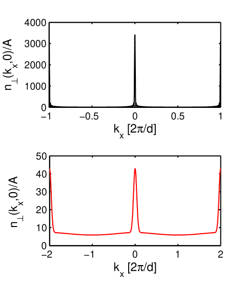
Figure 1: Planar momentum distribution for $k_{y}=0$. The upper panel is plotted for a uniform ideal gas with $N_{s}=10^{6}$ sites and one atom per site, and for a condensed fraction $f_{c}\sim 5$ %. The lower panel is plotted for our harmonic trap model with interactions (using $\alpha=0$), also for a condensed fraction $f_{c}\sim 5$ % and a total number $N=10^{6}$ using the trap parameters given in Gerbier et al. (2005b). Note the vastly different scales on the vertical axes.

Ideal gas in a harmonic trap -

As mentioned above, current experiments are carried out in the presence of a harmonic trap superimposed on the lattice. In this case, one expects the ground state wavefunction to be localized on a scale given by the harmonic potential ground state extension $\sigma_{\rm T}=\sqrt{\hbar/m\omega_{\rm T}}$, and not by the “number of lattice sites” (roughly equivalent to the size $w_{0}$ of the laser beams). In fact, usually one has $w_{0}\gg\sigma_{\rm T}$. The main point here is that the suppression factor is no longer hopelessly small, especially when most atoms are non-condensed. However, as well known, this ideal gas model for the condensate is a poor description of realistic experimental situations Dalfovo et al. (1999).

Interacting gas in a harmonic trap -

To obtain a better description, it is necessary to include interatomic interactions in the picture. In the Thomas-Fermi limit, which usually applies to experimental situations, the in-trap spatial condensate wavefunction will be significantly broader than in the ideal gas case, implying a narrower momentum distribution. However, as argued above, the post-expansion momentum profile can be very different from the sharply peaked in-trap profile. First, the interaction energy is released as kinetic expansion energy, and second, for a finite time-of-flight $t$ the initial size of the distribution is not necessarily negligible. Due to these effects, the actual momentum distribution will differ from the one calculated using Eq. (3).

Here, we handle them in a heuristic way, by approximating the maxima in the planar momentum distribution for the condensate as Gaussians,

$$n_{0}\left({\bf k}_{\perp}\approx{\bf K}_{\rm max}\right)\approx\frac{N_{0}\pi^{2}A}{(\Delta k_{\rm eff}d)^{2}}\exp\left(-{\bf k}_{\perp}^{2}/\Delta k_{\rm eff}^{2}\right).$$ (11)

We assume an effective spatial width given by the quadratic sum of the initial width $\sigma_{0}$ and of the expansion width $\hbar\Delta k_{0}/mt$ corresponding to the release energy. In momentum space, this corresponds to $\Delta k_{\rm eff}^{2}=\Delta k^{2}+\left(\frac{m\sigma_{0}}{\hbar t}\right)^{2}$. In the Thomas-Fermi limit, both the post-expansion momentum width $\Delta k$ and the initial size $\sigma_{0}$ are determined by the interaction energy, which itself is proportional to the chemical potential $\mu$. Accordingly, one has

$$\frac{\hbar^{2}\Delta k^{2}}{m} =\alpha\mu,\leavevmode\nobreak\ \leavevmode\nobreak\ m\omega_{T}^{2}\sigma_{0}^{2} =\beta\mu,$$ (12)

where the coefficients $\alpha$ and $\beta$ are of order unity. The final result is

$$\Delta k_{\rm eff}^{2}\approx\frac{m\mu}{\hbar^{2}}\left(\alpha+\frac{\beta}{(\omega_{T}t)^{2}}\right),$$ (13)

corresponding to a suppression factor $\left(\Delta k_{\rm eff}d\right)^{2}$ proportional to $\frac{md^{2}\mu}{\hbar^{2}}\sim\mu/E_{R}\lesssim 1$ much larger than expected from Eq. (10) (we estimate below the proportionality factor). Hence, one expects the observed visibility to follow the evolution of the condensed fraction at least qualitatively. The argument also holds for the quantum-depleted part of the non-condensed cloud.

Visibility for a trapped gas model

To make the preceding arguments more precise, we introduce a semiclassical description of the thermal cloud, for which interaction effects can usually be neglected to a first approximation Dalfovo et al. (1999). The thermal component is characterized by a distribution function in phase space given by

$$\rho({\bf r},{\bf k}) =\frac{1}{\exp\left[(\epsilon_{{\bf k}}+V(\bf{r})-\mu)/k_{\rm B}T\right]-1},$$ (14)

with the tight-binding dispersion relation $\epsilon_{{\bf k}}=2J\sum_{i=x,y,z}\left(1-\cos(k_{i}d)\right)$, with the trap potential $V({\bf r})=\frac{1}{2}m\omega_{T}^{2}r^{2}$. We can obtain the thermal fraction by integration over phase space,

$$N_{\rm th} =(2\pi)^{3/2}\left(\frac{R_{\rm th}}{d}\right)^{3}\sum_{n=1}^{\infty}\frac{e^{n(\mu-6J)/k_{\rm B}T}}{n^{3/2}}I_{0}\left(2nJ/k_{\rm B}T\right)^{3}.$$ (15)

Here $I_{0}$ is a Bessel function and $R_{\rm th}=\sqrt{\frac{k_{B}T}{m\omega_{T}^{2}}}$ the thermal cloud radius. The critical temperature for condensation follows from Eq. (15) by setting the chemical potential $\mu=0$ Dalfovo et al. (1999). Integrating the phase space distribution over position and $k_{z}$ gives the planar momentum distribution,

$$n_{\perp}({\bf k}_{\perp}) = A(2\pi)^{3/2}\left(\frac{R_{\rm th}}{d}\right)^{3}\sum_{n=1}^{\infty}\frac{e^{n(\mu-2J)/k_{\rm B}T}}{n^{3/2}}$$ (16)

$$I_{0}\left(2nJ/k_{\rm B}T\right)e^{-n\epsilon_{{\bf k}_{\perp}}/k_{\rm B}T}.$$

This takes the form announced in Eq. (8).

To estimate $\alpha$ and $\beta$ in Eq. (13), we impose that our Gaussian model should reproduce the same interaction and potential energy as a condensate in the Thomas-Fermi limit, with chemical potential given by Greiner (2003)

$$\mu=\left(\frac{15}{16\sqrt{2}\pi}N_{0}U\right)^{2/5}\left(m\omega_{T}^{2}d^{2}\right)^{2/5}.$$ (17)

The potential energy per particle Dalfovo et al. (1999) $E_{\rm pot}=\frac{3}{7}\mu=\frac{3}{4}m\omega_{T}^{2}\sigma_{0}^{2}$ gives a coefficient $\beta\approx 12/21$. The coefficient $\alpha$ depends on how the interaction energy is redistributed during the expansion. We consider the two limits, where the interaction energy is entirely concentrated either into the single diffraction peak under consideration ($E_{\rm int}=2\mu/7=3\hbar^{2}\Delta k_{0}^{2}/4m$, or $\alpha=8/21$), or in the central peak avoided by the visibility measurement ($\alpha=0$). This provides upper and lower bounds for the actual visibility. The results of the calculations is plotted in Fig. 2 for various assumptions: no trap, ideal gas in a trap, interacting gas in a trap with $\alpha=0$ or $\alpha=8/21$. Comparing the two latter cases, one sees that the final result depends sensitively on the value of $\alpha$. A more complete calculation would probably yield a curve lying in between the two bounds plotted. Nevertheless, irrespective of the particular model, the curves demonstrate that the visibility falls well below unity in a broad temperature range, where the condensate fraction stays non-zero.

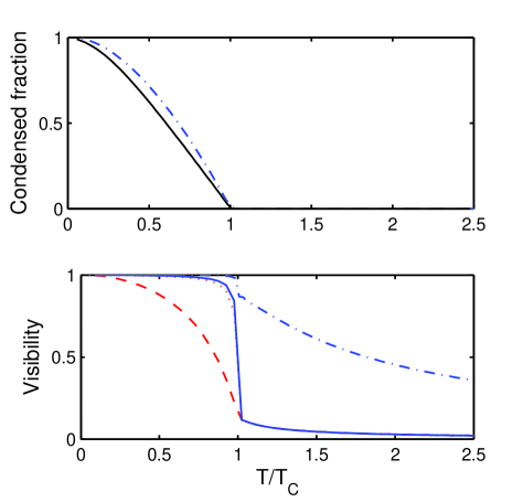
Figure 2: Upper plot: Calculated condensed fraction for an ideal Bose gas in a periodic potential, with and without additional harmonic trap. Lower plot: visibility of the interference observed after release from the trap. The dash-dotted line corresponds to an uniform ideal gas, as in the model of Diener et al. (2006), the solid line to a harmonically trapped ideal gas. The long and short-dashed lines correspond to two models of an interacting condensate, which should be seen as upper and lower bounds for the visibility ($\alpha=0$ and $\alpha=8/21$, see text). The curves are plotted for $N=10^{6}$ atoms, $V_{0}=10\leavevmode\nobreak\ E_{R}$ and an expansion time $t=20\leavevmode\nobreak\$ms.

In conclusion, we have calculated the visibility of the interference pattern observed when releasing a finite temperature, Bose-condensed gas from an optical lattice. Using a realistic model for the condensate momentum distribution, we find that the evolution of the visibility with temperature or lattice depth follows the evolution of the condensed fraction at least qualitatively. We therefore disagree with the conclusion made in Ref. Diener et al. (2006), that a measured visibility deviating from unity necessarily implies the absence of a Bose condensate in the system. This claim originates essentially from neglecting interaction effects on the gas expansion, which is a valid approximation close or in the Mott insulator regime, but a poor one for a system including a sizeable condensate, with or without Dalfovo et al. (1999) an optical lattice. We do however agree with the authors of Diener et al. (2006) on the importance of finite temperature effects in current experiments, as implied by recent experimental Stöferle et al. (2004); Gerbier et al. (2006); Fölling et al. (2006) and theoretical work DeMarco et al. (2005); Rey et al. (2006); Lu and Yu (2006); Capogrosso-Sansone et al. (2006); Gerbier (2007), and certainly consider this topic to warrant further investigations.

We would like to thank Martin Zwierlein for useful comments on the manuscript.