Superlight small bipolarons: a route to room temperature superconductivity

Abstract

Extending the BCS theory towards the strong electron-phonon interaction (EPI), a charged Bose liquid of small bipolarons has been predicted by us with a further prediction that the highest superconducting critical temperature is found in the crossover region of the EPI strength from the BCS-like to bipolaronic superconductivity. Later on we have shown that the unscreened (infinite-range) Fröhlich EPI combined with the strong Coulomb repulsion create superlight small bipolarons, which are several orders of magnitude lighter than small bipolarons in the Holstein-Hubbard model (HHM) with a zero-range EPI. The analytical and numerical studies of this Coulomb-Fröhlich model (CFM) provide the following recipes for room-temperature superconductivity: (a) The parent compound should be an ionic insulator with light ions to form high-frequency optical phonons, (b) The structure should be quasi two-dimensional to ensure poor screening of high-frequency phonons polarized perpendicular to the conducting planes, (c) A triangular lattice is required in combination with strong, on-site Coulomb repulsion to form the small superlight bipolaron, (d) Moderate carrier densities are required to keep the system of small bipolarons close to the Bose-Einstein condensation regime. Clearly most of these conditions are already met in the cuprates.

I Introduction

The discovery of high-temperature superconductivity in cuprates bed has widened significantly our horizons of the theoretical understanding of the physical phenomenon. A great number of observations point to the possibility that the cuprate superconductors may not be conventional Bardeen-Cooper-Schrieffer (BCS) superconductors bcs , but rather derive from the Bose-Einstein condensation (BEC) of real-space small bipolarons alemot ; alebook ; edwards . Importantly a first proposal for high temperature superconductivity by Ogg Jr in 1946 ogg , already involved real-space pairing of individual electrons into bosonic molecules with zero total spin. This idea was further developed as a natural explanation of conventional superconductivity by Schafroth sha and Butler and Blatt blatt . Unfortunately the Ogg-Schafroth picture was practically forgotten because it neither accounted quantitatively for the critical behavior of conventional superconductors, nor did it explain the microscopic nature of attractive forces which could overcome the Coulomb repulsion between two electrons constituting a pair. On the contrary highly successful for low-$T_{c}$ metals and alloys the BCS theory, where two electrons were indeed correlated, but at a very large distance of about $10^{3}$ times of the average inter-electron spacing, led many researchers to believe that any superconductor is a ”BCS-like”.

However it has been found— unexpectedly for many researchers— that the BCS theory and its extension eli towards the intermediate coupling regime, $\lambda\lesssim 1$, break down already at $\lambda\gtrsim 1$ ale0 . It happens since the Migdal ”noncrossing” approximation mig of the theory is not applied at $\lambda\gtrsim 1$. In fact, the small parameter of the theory, $\lambda\omega_{0}/E_{F}$, becomes large at $\lambda\gtrsim 1$ because the bandwidth is narrowed and the Fermi energy, $E_{F}$ is renormalised down exponentially due to the small polaron formation ale0 ; alexandrov:2001 (here $\omega_{0}$ is the characteristic phonon frequency, and we take $\hbar=c=k_{B}=1$). Extending the BCS theory towards the strong interaction between electrons and ion vibrations, $\lambda\gg 1$, a charged Bose gas of tightly bound small bipolarons was predicted aleran instead of Cooper pairs, with a further prediction that the highest superconducting transition temperature is attained in the crossover region of EPI strength, $\lambda\thickapprox 1$, between the BCS and bipolaronic superconductivity ale0 .

For a very strong EPI polarons become self-trapped on a single lattice site and bipolarons are on-site singlets. A finite on-site bipolaron mass appears only in the second order of polaron hopping, aleran , so that on-site bipolarons might be very heavy in HHM, where EPI is short-ranged. Actually HHM led some authors to the conclusion that the formation of itinerant small polarons and bipolarons in real materials is unlikely mel , and high-temperature bipolaronic superconductivity is impossible and2 . Nevertheless treating the onsite repulsion (Hubbard $U$) and the short-range EPI on an equal footing led several authors to the opposite conclusion with respect to bipolaron mobility even in HHM, which is generally unfavorable for coherent tunnelling. Aubry aub93 found along with the onsite bipolaron ($S0$) also an anisotropic pair of polarons lying on two neighboring sites (i.e. the $intersite$ bipolaron, $S1$) with classical phonons in the extreme adiabatic limit. Such bipolarons were originally hypothesized in alexandrov:1991 ; alegap to explain the anomalous nuclear magnetic relaxation (NMR) in cuprate superconductors. The intersite bipolaron could take a form of a ”quadrisinglet” ($QS$) in 2D HHM, where the electron density at the central site is 1 and ”1/4” on the four nearest neigbouring sites. In a certain region of $U$, where $QS$ is the ground state, the double-well potential barrier which usually pins polarons and bipolarons to the lattice depresses to almost zero, so that adiabatic lattice bipolarons can be rather mobile.

Mobile $S1$ bipolarons were found in 1D HHM using variational methods also in the non and near-adiabatic regimes with dynamical quantum phonons lamagna ; trugman . The intersite bipolaron with a relatively small effective mass is stable in a wide region of the parameters of HHM due to both exchange and nonadiabaticity effects lamagna . Near the strong coupling limit the mobile $S1$ bipolaron has an effective mass of the order of a single Holstein polaron mass, so that one should not rule out the possibility of a superconducting state of $S1$ bipolarons with $s$ or $d$-wave symmetry in HHM trugman . More recent diagrammatic Monte Carlo study Macridin found $S1$ bipolarons for large $U$ at intermediate and large EPI and established the phase diagram of 2D HHM, comprising unbound polarons, $S0$ and $S1$ domains. Ref. Macridin emphasised that the transition to the bound state and the properties of the bipolaron in HHM are very different from bound states in the attractive (negative $U$) Hubbard model without EPI micnas1981 .

In any case the Holstein model is an extreme polaron model, with typically highest possible values of the (bi)polaron mass in the strong coupling regime ale5 ; alekor ; spencer ; jim . Many doped ionic lattices, including cuprates, are characterized by poor screening of high-frequency optical phonons and they are more appropriately described by the finite-range Fröhlich EPI. The unscreened Fröhlich EPI provides relatively light lattice polarons and combined with the Coulomb repulsion also ”superlight” but yet small (intersite) bipolarons. In contrast with the crawler motion of on-site bipolarons, the intersite-bipolaron tunnelling is a crab-like, so that the effective mass scales linearly with the polaron mass. Such bipolarons are several orders of magnitude lighter than small bipolarons in HHM ale5 . Here I review a few analytical ale5 ; alekor2 and more recent Quantum Monte-Carlo (QMC) jim2 ; jim3 studies of CFM which have found superlight bipolarons in a wide parameter range with achievable phonon frequencies and couplings. They could have a superconducting transition in excess of room temperature.

II Coulomb-Fröhlich model

Any realistic theory of doped narrow-band ionic insulators should include both the finite-range Coulomb repulsion and the strong finite-range EPI. From a theoretical standpoint, the inclusion of the finite-range Coulomb repulsion is critical in ensuring that the carriers would not form clusters. The Coulomb repulsion, $V_{c}$, makes the clusters unstable and lattice bipolarons more mobile.

To illustrate the point let us consider a generic multi-polaron ”Coulomb-Fröhlich” model (CFM) on a lattice, which explicitly includes the finite-range Coulomb repulsion, $V_{c}$, and the strong long-range EPI ale5 ; alekor2 . The implicitly present (infinite) Hubbard $U$ prohibits double occupancy and removes the need to distinguish the fermionic spin, if we are interested in the charge rather than spin excitations. Introducing spinless fermion operators $c_{{\bf n}}$ and phonon operators $d_{{\bf m}}$, the Hamiltonian of CFM is written in the real-space representation as alekor2

$$H = \sum_{{\bf n\neq n^{\prime}}}T({\bf n-n^{\prime}})c_{{\bf n}}^{\dagger}c_{{\bf n^{\prime}}}+{1\over{2}}\sum_{{\bf n\neq n^{\prime}}}V_{c}({\bf n-n^{\prime}})c_{{\bf n}}^{\dagger}c_{{\bf n}}c_{{\bf n^{\prime}}}^{\dagger}c_{{\bf n^{\prime}}}+$$

$$\omega_{0}\sum_{{\bf n\neq m}}g({\bf m-n})({\bf e}\cdot{\bf e}_{{\bf m-n}})c_{{\bf n}}^{\dagger}c_{{\bf n}}(d_{{\bf m}}^{\dagger}+d_{{\bf m}})+$$

$$\omega_{0}\sum_{{\bf m}}\left(d_{{\bf m}}^{\dagger}d_{{\bf m}}+\frac{1}{2}\right),$$

where $T({\bf n})$ is the bare hopping integral in a rigid lattice. In general, this many-body model is of considerable complexity. However, if we are interested in the non or near adiabatic limit and the strong EPI, the kinetic energy is a perturbation. Then the model can be grossly simplified using the Lang-Firsov canonical transformation lan in the Wannier representation for electrons and phonons,

$$S=\sum_{{\bf m\neq n}}g({\bf m-n})({\bf e}\cdot{\bf e}_{{\bf m-n}})c_{{\bf n}}^{\dagger}c_{{\bf n}}(d_{{\bf m}}^{\dagger}-d_{{\bf m}}).$$

Here we consider a particular lattice structure, where intersite lattice bipolarons tunnel already in the first order in $T({\bf n})$. That allows us to average the transformed Hamiltonian, $\tilde{H}=\exp(S)H\exp(-S)$ over phonons to obtain

$$\tilde{H}=H_{0}+H_{pert},$$ (2)

where

$$H_{0}=-E_{p}\sum_{{\bf n}}c_{{\bf n}}^{\dagger}c_{{\bf n}}+{1\over{2}}\sum_{{\bf n\neq n^{\prime}}}v({\bf n-n^{\prime}})c_{{\bf n}}^{\dagger}c_{{\bf n}}c_{{\bf n^{\prime}}}^{\dagger}c_{{\bf n^{\prime}}}+\omega_{0}\sum_{{\bf m}}\left(d_{{\bf m}}^{\dagger}d_{{\bf m}}+\frac{1}{2}\right),$$

and

$$H_{pert}=\sum_{{\bf n\neq n^{\prime}}}t({\bf n-n^{\prime}})c_{{\bf n}}^{\dagger}c_{{\bf n^{\prime}}}.$$

is a perturbation. $E_{p}$ is the familiar polaron level shift,

$$E_{p}=\omega_{0}\sum_{{\bf m}\nu}g^{2}({\bf m-n})({\bf e}\cdot{\bf e}_{{\bf m-n}})^{2},$$ (3)

which is independent of ${\bf n}$. The polaron-polaron interaction is

$$v({\bf n-n^{\prime}})=V_{c}({\bf n-n^{\prime}})-V_{ph}({\bf n-n^{\prime}}),$$ (4)

where

$$V_{ph}({\bf n-n^{\prime}})=2\omega_{0}\sum_{\bf m}g({\bf m-n})g({\bf m-n^{\prime}})({\bf e}\cdot{\bf e}_{{\bf m-n}})({\bf e}\cdot{\bf e}_{{\bf m-n^{\prime}}}).$$ (5)

The transformed hopping integral is $t({\bf n-n^{\prime}})=T({\bf n-n^{\prime}})\exp[-g^{2}({\bf n-n^{\prime}})]$ with

$$g^{2}({\bf n-n^{\prime}}) = \sum_{{\bf m},\nu}g({\bf m-n})({\bf e}\cdot{\bf e}_{{\bf m-n}})\times$$

$$\left[g({\bf m-n})({\bf e}\cdot{\bf e}_{{\bf m-n}})-g({\bf m-n^{\prime}})({\bf e}\cdot{\bf e}_{{\bf m-n^{\prime}}})\right]$$

at low temperatures. The mass renormalization exponent can be expressed via $E_{p}$ and $V_{ph}$ as

$$g^{2}({\bf n-n^{\prime}})=\frac{1}{\omega_{0}}\left[E_{p}-\frac{1}{2}V_{ph}({\bf n-n^{\prime}})\right].$$ (7)

The Hamiltonian $\tilde{H}$, Eq.(2), in zero order with respect to the hopping describes localised polarons and independent phonons, which are vibrations of ions relative to new equilibrium positions depending on the polaron occupation numbers. Importantly the phonon frequencies remain unchanged in this limit at any polaron density, $n$. At finite $\lambda$ and $n$ there is a softening of phonons $\delta\omega_{0}$ of the order of $\omega_{0}n/\lambda^{2}$ ale2 . Interestingly the optical phonon can be mixed with a low-frequency polaronic plasmon forming a new excitation, ”plasphon”, which was proposed in plasphon ; ale2 as an explanation of the anomalous phonon mode splitting observed in cuprates splitting . The middle of the electron band is shifted down by the polaron level-shift $E_{p}$ due to the potential well created by lattice deformation.

When $V_{ph}$ exceeds $V_{c}$ the full interaction becomes negative and polarons form pairs. The real space representation allows us to elaborate more physics behind the lattice sums in $V_{ph}$ alekor2 . When a carrier (electron or hole) acts on an ion with a force ${\bf f}$, it displaces the ion by some vector ${\bf x}={\bf f}/k$. Here $k$ is the ion’s force constant. The total energy of the carrier-ion pair is $-{\bf f}^{2}/(2k)$. This is precisely the summand in Eq.(3) expressed via dimensionless coupling constants. Now consider two carriers interacting with the same ion. The ion displacement is ${\bf x}=({\bf f}_{1}+{\bf f}_{2})/k$ and the energy is $-{\bf f}_{1}^{2}/(2k)-{\bf f}_{2}^{2}/(2k)-({\bf f}_{1}\cdot{\bf f}_{2})/k$. Here the last term should be interpreted as an ion-mediated interaction between the two carriers. It depends on the scalar product of ${\bf f}_{1}$ and ${\bf f}_{2}$ and consequently on the relative positions of the carriers with respect to the ion. If the ion is an isotropic harmonic oscillator, then the following simple rule applies. If the angle $\phi$ between ${\bf f}_{1}$ and ${\bf f}_{2}$ is less than $\pi/2$ the polaron-polaron interaction will be attractive, if otherwise it will be repulsive. In general, some ions will generate attraction, and some repulsion between polarons.

The overall sign and magnitude of the interaction is given by the lattice sum in Eq.(5). One should note that according to Eq.(7) an attractive EPI reduces the polaron mass (and consequently the bipolaron mass), while repulsive EPI enhances the mass. Thus, the long-range EPI serves a double purpose. Firstly, it generates an additional inter-polaron attraction because the distant ions have small angle $\phi$. This additional attraction helps to overcome the direct Coulomb repulsion between polarons. And secondly, the Fröhlich EPI makes lattice (bi)polarons lighter. Here, following ale5 ; alekor2 ; jim2 ; jim3 , we consider a few examples of intersite superlight bipolarons.

III Apex bipolarons

High-$T_{c}$ oxides are doped charged-transfer ionic insulators with narrow electron bands. Therefore, the interaction between holes can be analyzed using computer simulation techniques based on a minimization of the ground state energy of an ionic insulator with two holes, the lattice deformations and the Coulomb repulsion fully taken into account, but neglecting the kinetic energy terms. Using these techniques net inter-site interactions of the in-plane oxygen hole with the $apex$ hole, Fig.1, and of two in-plane oxygen holes, Fig.2, were found to be attractive in $La_{2}CuO_{4}$ cat with the binding energies $\Delta=119meV$ and $\Delta=60meV$, respectively. All other interactions were found to be repulsive.

Both apex and in-plane bipolarons can tunnel from one unit cell to another via the  single-polaron tunnelling from one apex oxygen to its apex neighbor in case of the apex bipolaron ale5 , Fig.1, or via the next-neighbor hopping in case of the in-plane bipolaron alekor2 , Fig.2.

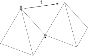
Figure 1: Apex bipolaron tunnelling in perovskites (after ale5 )

The Bloch bands of these bipolarons are obtained using the canonical transformation, described above, projecting the transformed Hamiltonian, Eq.(2), onto a reduced Hilbert space containing only empty or doubly occupied elementary cells alebook . The wave function of the apex bipolaron localized, say in cell ${\bf m}$ is written as

$$|{\bf m}\rangle=\sum_{i=1}^{4}A_{i}c_{i}^{\dagger}c_{apex}^{\dagger}|0\rangle,$$ (8)

where $i$ denotes the $p_{x,y}$ orbitals and spins of the four plane oxygen ions in the cell, Fig.1, and $c_{apex}^{\dagger}$ is the creation operator for the hole in one of the three apex oxygen orbitals with the spin, which is the same or opposite to the spin of the in-plane hole depending on the total spin of the bipolaron. The probability amplitudes $A_{i}$ are normalized by the condition $|A_{i}|=1/2,$ if four plane orbitals $p_{x1},p_{y2},p_{x3}$ and $p_{y4}$ are involved, or by $|A_{i}|=1/\sqrt{2}$ if only two of them are relevant. Then a matrix element of the Hamiltonian Eq.(2) describing the bipolaron tunnelling to the nearest neighbor cell ${\bf m+a}$ is found as

$$t_{b}=\langle{\bf m}|\tilde{H}|{\bf m}+{\bf a}\rangle=|A_{i}|^{2}T_{pp^{\prime}}^{apex}e^{-g^{2}},$$ (9)

where $T_{pp^{\prime}}^{apex}e^{-g^{2}}$ is a single polaron hopping integral between two apex ions. The inter-site bipolaron tunnelling appears already in the first order with respect to the single-hole transfer $T_{pp^{\prime}}^{apex}$, and the bipolaron energy spectrum consists of two subbands $E^{x,y}({\bf K),}$ formed by the overlap of $p_{x}$ and $p_{y}$ $apex$ oxygen orbitals, respectively (here we take the lattice constant $a=1$):

$$E^{x}({\bf K}) = t\cos(K_{x})-t^{\prime}\cos(K_{y}),$$ (10)

$$E^{y}({\bf K}) = -t^{\prime}\cos(K_{x})+t\cos(K_{y}).$$

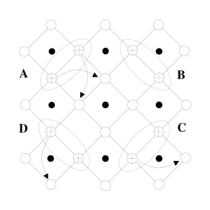
Figure 2: Four degenerate in-plane bipolaron configurations A, B, C, and D . Some single-polaron hoppings are indicated by arrows (Reproduced from A. S. Alexandrov and P. E. Kornilovitch, J. Phys.: Condens. Matter 14, 5337 (2002), (c) IOP Publishing Limited, 2007. alekor2 ).

They transform into one another under $\pi/2$ rotation. If $t,t^{\prime}>0,$ “$x"$ bipolaron band has its minima at ${\bf K=}(\pm\pi,0)$ and $y$-band at ${\bf K}=(0,\pm\pi)$. In these equations $t$ is the renormalized hopping integral between $p$ orbitals of the same symmetry elongated in the direction of the hopping ($pp\sigma$) and $t^{\prime}$ is the renormalized hopping integral in the perpendicular direction ($pp\pi$). Their ratio $t/t^{\prime}=T_{pp^{\prime}}^{apex}/T^{\prime}{}_{pp^{\prime}}^{apex}=4$ as follows from the tables of hopping integrals in solids. Two different bands are not mixed because $T_{p_{x},p_{y}^{\prime}}^{apex}=0$ for the nearest neighbors. A random potential does not mix them either, if it varies smoothly on the lattice scale. Hence, we can distinguish ‘$x$’ and ‘$y$’ bipolarons with a lighter effective mass in $x$ or $y$ direction, respectively. The apex $z$ bipolaron, if formed, is $ca.$ four times less mobile than $x$ and $y$ bipolarons. The bipolaron bandwidth is of the same order as the polaron one, which is a specific feature of the inter-site bipolaron. For a large part of the Brillouin zone near $(0,\pi)$ for ‘$x$’ and $(\pi,0)$ for ‘$y$’ bipolarons, one can adopt the effective mass approximation

$$E^{x,y}({\bf K})={\frac{K_{x}^{2}}{{2m_{x,y}^{\ast\ast}}}}+{\frac{K_{y}^{2}}{{2m_{y,x}^{\ast\ast}}}}$$ (11)

with $K_{x,y}$ taken relative to the band bottom positions and $m_{x}^{\ast\ast}=1/t$, $m_{y}^{\ast\ast}=4m_{x}^{\ast\ast}$.

$X$ and $y$ bipolarons bose-condense at the boundaries of the center-of-mass Brillouin zone with $K=(\pm\pi,0)$ and $K=(0,\pm\pi)$, respectively, which explains the d-wave symmetry and the checkerboard modulations of the order parameter in cuprates aledwave .

IV In-plane bipolarons

Now let us consider in-plane bipolarons in a two-dimensional lattice of ideal octahedra that can be regarded as a simplified model of the copper-oxygen perovskite layer, Fig.3 alekor2 . The lattice period is $a=1$ and the distance between the apical sites and the central plane is $h=a/2=0.5$. For mathematical transparency we assume that all in-plane atoms, both copper and oxygen, are static but apex oxygens are independent three-dimensional isotropic harmonic oscillators.

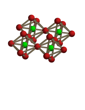
Figure 3: Simplified model of the copper-oxygen perovskite layer. Reproduced from A. S. Alexandrov and P. E. Kornilovitch, J. Phys.: Condens. Matter 14, 5337 (2002), (c) IOP Publishing Limited, 2007. alekor2

Due to poor screening, the hole-apex interaction is purely coulombic,

$$g_{\alpha}({\bf m-n})=\frac{\kappa_{\alpha}}{|{\bf m-n}|^{2}},$$

where $\alpha=x,y,z$. To account for the fact that $c$ axis-polarized phonons couple to the holes stronger than others due to a poor screening ale5 ; alekor ; alekor2 , we choose $\kappa_{x}=\kappa_{y}=\kappa_{z}/\sqrt{2}$. The direct hole-hole repulsion is

$$V_{c}({\bf n-n^{\prime}})=\frac{V_{c}}{\sqrt{2}|{\bf n-n^{\prime}}|}$$

so that the repulsion between two holes in the nearest neighbor ($NN$) configuration is $V_{c}$. We also include the bare $NN$ hopping $T_{NN}$, the next nearest neighbor ($NNN$) hopping across copper $T_{NNN}$ and the $NNN$ hopping between the pyramids $T_{NNN}^{\prime}$.

The polaron shift is given by the lattice sum Eq.(3), which after summation over polarizations yields

$$E_{p}=2\kappa_{x}^{2}\omega_{0}\sum_{{\bf m}}\left(\frac{1}{|{\bf m-n}|^{4}}+\frac{h^{2}}{|{\bf m-n}|^{6}}\right)=31.15\kappa_{x}^{2}\omega_{0},$$ (12)

where the factor $2$ accounts for two layers of apical sites. For reference, the Cartesian coordinates are ${\bf n}=(n_{x}+1/2,n_{y}+1/2,0)$, ${\bf m}=(m_{x},m_{y},h)$, and $n_{x},n_{y},m_{x},m_{y}$ are integers. The polaron-polaron attraction is

$$V_{ph}({\bf n-n^{\prime}})=4\omega\kappa_{x}^{2}\sum_{{\bf m}}\frac{h^{2}+({\bf m-n^{\prime}})\cdot({\bf m-n})}{|{\bf m-n^{\prime}}|^{3}|{\bf m-n}|^{3}}.$$ (13)

Performing the lattice summations for the $NN$, $NNN$, and $NNN^{\prime}$ configurations one finds $V_{ph}=1.23\,E_{p},$ $0.80\,E_{p}$, and $0.82\,E_{p}$, respectively. As a result, we obtain a net inter-polaron interaction as $v_{NN}=V_{c}-1.23\,E_{p}$, $v_{NNN}=\frac{V_{c}}{\sqrt{2}}-0.80\,E_{p}$, $v_{NNN}^{\prime}=\frac{V_{c}}{\sqrt{2}}-0.82\,E_{p}$, and the mass renormalization exponents as $g_{NN}^{2}=0.38(E_{p}/\omega)$, $g_{NNN}^{2}=0.60(E_{p}/\omega)$ and $(g^{\prime}{}_{NNN})^{2}=0.59(E_{p}/\omega)$.

Let us now discuss different regimes of the model. At $V_{c}>1.23\,E_{p}$, no bipolarons are formed and the system is a polaronic Fermi liquid. Polarons tunnel in the square lattice with $t=T_{NN}\exp(-0.38E_{p}/\omega)$ and $t^{\prime}=T_{NNN}\exp(-0.60E_{p}/\omega)$ for $NN$ and $NNN$ hoppings, respectively. Since $g_{NNN}^{2}\approx(g_{NNN}^{\prime})^{2}$ one can neglect the difference between $NNN$ hoppings within and between the octahedra. A single polaron spectrum is therefore

$$E_{1}({\bf k})=-E_{p}-2t^{\prime}[\cos k_{x}+\cos k_{y}]-4t\cos(k_{x}/2)\cos(k_{y}/2).$$ (14)

The polaron mass is $m^{\ast}=1/(t+2t^{\prime})$. Since in general $t>t^{\prime}$, the mass is mostly determined by the $NN$ hopping amplitude $t$.

If $V_{c}<1.23\,E_{p}$ then intersite $NN$ bipolarons form. The bipolarons tunnel in the plane via four resonating (degenerate) configurations $A$, $B$, $C$, and $D$, as shown in Fig.2. In the first order of the renormalized hopping integral, one should retain only these lowest energy configurations and discard all the processes that involve configurations with higher energies. The result of such a projection is the bipolaron Hamiltonian,

$$H_{b} = (V_{c}-3.23\,E_{p})\sum_{{\bf l}}[A_{{\bf l}}^{\dagger}A_{{\bf l}}+B_{{\bf l}}^{\dagger}B_{{\bf l}}+C_{{\bf l}}^{\dagger}C_{{\bf l}}+D_{{\bf l}}^{\dagger}D_{{\bf l}}]$$

$$-t^{\prime}\sum_{{\bf l}}[A_{{\bf l}}^{\dagger}B_{{\bf l}}+B_{{\bf l}}^{\dagger}C_{{\bf l}}+C_{{\bf l}}^{\dagger}D_{{\bf l}}+D_{{\bf l}}^{\dagger}A_{{\bf l}}+H.c.]$$

$$-t^{\prime}\sum_{{\bf n}}[A_{{\bf l-x}}^{\dagger}B_{{\bf l}}+B_{{\bf l+y}}^{\dagger}C_{{\bf l}}+C_{{\bf l+x}}^{\dagger}D_{{\bf l}}+D_{{\bf l-y}}^{\dagger}A_{{\bf l}}+H.c.],$$

where ${\bf l}$ numbers octahedra rather than individual sites, ${\bf x}=(1,0)$, and ${\bf y}=(0,1)$. A Fourier transformation and diagonalization of a $4\times 4$ matrix yields the bipolaron spectrum:

$$E_{2}({\bf K})=V_{c}-3.23E_{p}\pm 2t^{\prime}[\cos(K_{x}/2)\pm\cos(K_{y}/2)].$$ (16)

There are four bipolaronic subbands combined in the band of the width $8t^{\prime}$. The effective mass of the lowest band is $m^{\ast\ast}=2/t^{\prime}$. The bipolaron binding energy is $\Delta\approx 1.23E_{p}-V_{c}.$ Inter-site bipolarons already move in the first order of the single polaron hopping. This remarkable property is entirely due to the strong on-site repulsion and long-range electron-phonon interactions that leads to a non-trivial connectivity of the lattice. This fact combines with a weak renormalization of $t^{\prime}$ yielding a superlight bipolaron with the mass $m^{\ast\ast}\propto\exp(0.60\,E_{p}/\omega)$. We recall that in the Holstein model $m^{\ast\ast}\propto\exp(2E_{p}/\omega)$ aleran . Thus the mass of the Fröhlich bipolaron in the perovskite layer scales approximately as a cubic root of that of the Holstein bipolaron.

At even stronger EPI, $V_{c}<1.16E_{p}$, $NNN$ bipolarons become stable. More importantly, holes can now form 3- and 4-particle clusters. The dominance of the potential energy over kinetic in the transformed Hamiltonian enables us to readily investigate these many-polaron cases. Three holes placed within one oxygen square have four degenerate states with the energy $2(V_{c}-1.23E_{p})+V_{c}/\sqrt{2}-0.80E_{p}$. The first-order polaron hopping processes mix the states resulting in a ground state linear combination with the energy $E_{3}=2.71V_{c}-3.26E_{p}-\sqrt{4t^{2}+t^{\prime}{}^{2}}$. It is essential that between the squares such triads could move only in higher orders of polaron hopping. In the first order, they are immobile. A cluster of four holes has only one state within a square of oxygen atoms. Its energy is $E_{4}=4(V_{c}-1.23E_{p})+2(V_{c}/\sqrt{2}-0.80E_{p})=5.41V_{c}-6.52E_{p}$. This cluster, as well as all bigger ones, are also immobile in the first order of polaron hopping. We would like to stress that at distances much larger than the lattice constant the polaron-polaron interaction is always repulsive, and the formation of infinite clusters, stripes or strings is prohibited. We conclude that at $V_{c}<1.16E_{p}$ the system quickly becomes a charge segregated insulator.

The fact that within the window, $1.16E_{p}<V_{c}<1.23E_{p}$, there are no three or more polaron bound states, indicates that bipolarons repel each other. The system is effectively a charged Bose-gas, which is a superconductor ogg ; sha . This superconducting state requires a rather fine balance between electronic and ionic interactions in cuprates.

V All-coupling lattice bipolarons

The multi-polaron CFM model discussed above is analytically solvable in the strong-coupling nonadibatic ($\omega_{0}\gtrsim T(a))$ limit using the Lang-Firsov transformation of the Hamiltonian, Eq.(1), and projecting it on the inter-site pair Hilbert space ale5 ; alekor2 . To extend the theory for the whole parameter space an advanced continuous time QMC technique (CTQMC) has been recently developed for bipolarons jim2 ; jim3 . Using CTQMC refs. jim2 ; jim3 simulated the CFM Hamiltonian on a staggered triangular ladder (1D), triangular (2D) and strongly anisotropic hexagonal (3D) lattices including triplet pairing jim3 . On such lattices, bipolarons are found to move with a crab like motion (Fig. 1), which is distinct from the crawler motion found on cubic lattices aleran . Such bipolarons are small but very light for a wide range of electron-phonon couplings and phonon frequencies. EPI has been modeled using the force function in the site-representation as

$$H_{e-ph}=-\sum_{\mathbf{n}\mathbf{m}\sigma}f_{\mathbf{m}}(\mathbf{n})c^{\dagger}_{\mathbf{n}\sigma}c_{\mathbf{n}\sigma}\xi_{\mathbf{m}}\>.$$ (17)

Each vibrating ion has one phonon degree of freedom $\xi_{\mathbf{m}}$ associated with a single atom. The sites are numbered by the indices $\mathbf{n}$ or $\mathbf{m}$ for electrons and ions respectively. Operators $c^{\dagger}_{\mathbf{n}\sigma}$ creates an electron on site ${\bf n}$ with spin $\sigma$. Coulomb repulsion $V(\mathbf{n}-\mathbf{n}^{\prime})$ has been screened up to the first nearest neighbors, with on site repulsion $U$ and nearest-neighbor repulsion $V_{c}$. In contrast, the Fröhlich interaction is assumed to be long-range, due to unscreened interaction with c-axis high-frequency phonons ale5 . The form of the interaction with c-axis polarized phonons has been specified via the force functionalekor , $f_{\mathbf{m}}(\mathbf{n})=\kappa\left[(\mathbf{m}-\mathbf{n})^{2}+1\right]^{-3/2}$, where $\kappa$ is a constant. The dimensionless electron-phonon coupling constant $\lambda$ is defined as $\lambda=\sum_{\mathbf{m}}f^{2}_{\mathbf{m}}(0)/2M\omega^{2}zT(a)$ which is the ratio of the polaron binding energy to the kinetic energy of the free electron $zT(a)$, and the lattice constant is taken as $a=1$.

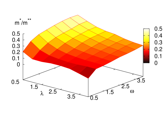
Figure 4: Polaron to bipolaron mass ratio for a range of $\bar{\omega}=\omega_{0}/T(a)$ and $\lambda$ on the staggered ladder. Mobile small bipolarons are seen even in the adiabatic regime $\bar{\omega}=0.5$ for couplings $\lambda$ up to 2.5 (Reproduced from J. P. Hague et al., Phys. Rev. Lett 98, 037002 (2007), (c) American Physical Society, 2007. jim2 ” ).

In the limit of high phonon frequency $\omega\gg T(a)$ and large on-site Coulomb repulsion (Hubbard $U$), the model is reduced to an extended Hubbard model with intersite attraction and suppressed double-occupancy alekor2 by applying the Lang-Firsov canonical transformation (section 2). Then the Hamiltonian can be projected onto the subspace of nearest neighbor intersite crab bipolarons (sections 4). In contrast with the crawler bipolaron, the crab bipolaron’s mass scales linearly with the polaron mass ($m^{**}=4m^{*}$ on the staggered chain and $m^{**}=6m^{*}$ on the triangular lattice).

Extending the CTQMC algorithm to systems of two particles with strong EPI and Coulomb repulsion solved the bipolaron problem on a staggered ladder, triangular and anisotropic hexagonal lattices from weak to strong coupling in a realistic parameter range where usual strong and weak-coupling limiting approximations fail. Importantly small but light bipolarons have been found for more realistic intermediate values of EPI, $\lambda\lesssim 1$ and phonon frequency, $\omega\lesssim T(a)$ jim2 ; jim3 .

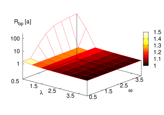
Figure 5: Bipolaron radius (in units of $a$) for a range of $\bar{\omega}$ and $\lambda$ on the staggered ladder (Reproduced from J. P. Hague et al., Phys. Rev. Lett 98, 037002 (2007), (c) American Physical Society, 2007. jim2 ” ).

Figure 4 shows the ratio of the polaron to bipolaron masses on the staggered ladder as a function of effective coupling and phonon frequency for $V_{c}=0$. The bipolaron to polaron mass ratio is about 2 in the weak coupling regime ($\lambda\ll 1$) as it should be for a large bipolaron ver . In the strong-coupling, large phonon frequency limit the mass ratio approaches 4, in agreement with strong-coupling arguments given above. In a wide region of parameter space, we find a bipolaron/polaron mass ratio of between 2 and 4 and a bipolaron radius similar to the lattice spacing, see Figs. 4 and 5. Thus the bipolaron is small and light at the same time. Taking into account additional intersite Coulomb repulsion $V_{c}$ does not change this conclusion. The bipolaron is stable for $V_{c}<4T(a)$. As $V_{c}$ increases the bipolaron mass decreases but the radius remains small, at about 2 lattice spacings. Importantly, the absolute value of the small bipolaron mass is only about 4 times of the bare electron mass $m_{0}$, for $\lambda=\omega/T(a)=1$ (see Fig. 4).

Simulations of the bipolaron on an infinite triangular lattice including exchanges and large on-site Hubbard repulsion $U=20T(a)$ also lead to the bipolaron mass of about $6m_{0xy}$ and the bipolaron radius $R_{bp}\thickapprox 2a$ for a moderate coupling $\lambda=0.5$ and a large phonon frequency $\omega=T(a)$ (for the triangular lattice, $m_{0xy}=1/3a^{2}T(a)$). Finally, the bipolaron in a hexagonal lattice with out-of-plane hopping $T^{\prime}=T(a)/3$ has also a light in-plane inverse mass, $m_{xy}^{**}\thickapprox 4.5m_{0xy}$ but a small size, $R_{bp}\thickapprox 2.6a$ for experimentally achievable values of the phonon frequency $\omega=T(a)=200$meV and EPI, $\lambda=0.36$. Out-of-plane $m_{z}^{**}\thickapprox 70m_{0z}$ is Holstein like, where $m_{0z}=1/2d^{2}T^{\prime}$, ($d$ is the inter-plane spacing). When bipolarons are small and pairs do not overlap, the pairs can form a BEC at $T_{BEC}=3.31(2n_{B}/a^{2}\sqrt{3}d)^{2/3}/(m_{xy}^{2/3}m_{z}^{1/3})$. If we choose realistic values for the lattice constants of 0.4 nm in the plane and 0.8 nm out of the plane, and allow the density of bosons to be $n_{B}$=0.12 per lattice site, which easily avoids overlap of pairs, then $T_{BEC}\thickapprox$ 300K.

VI Summary

For a very strong electron-phonon coupling in the Holstein model with the zero-range EPI, polarons become self-trapped on a single lattice site and bipolarons are on-site singlets. The on-site bipolaron mass appears only in the second order of polaron hopping aleran , so that on-site bipolarons are very heavy. This estimate led some authors to the conclusion that high-temperature bipolaronic superconductivity is impossible .

However we have found that small but relatively light bipolarons could exist within the realistic range of the finite-range EPI with high-frequency optical phonons. The effect appears since the finite-range Fröhlich interaction combined with the long-range Coulomb repulsion provides an effective interaction with a deep attraction minimum for two holes on the neighbouring sites, and repulsive for other hole configurations. Bipolarons which are both light and small give rise to Ogg-Schafroth’s bose-condensed state of charged bosons at high-temperatures, since the Bose-Einstein condensate has transition temperature that is inversely proportional to mass. Our conclusion is backed up by analytical ale5 ; alekor2 and CTQMC studies jim2 ; jim3 . These studies let us believe that the following recipes is worth investigating to look for room-temperature superconductivity jim2 : (a) The parent compound should be an ionic insulator with light ions to form high-frequency optical phonons, (b) The structure should be quasi two-dimensional to ensure poor screening of high-frequency phonons polarized perpendicular to the conducting planes, (c) A triangular lattice is required in combination with strong, on-site Coulomb repulsion to form the small superlight crab bipolaron, (d) Moderate carrier densities are required to keep the system of small bipolarons close to the dilute regime. Clearly most of these conditions are already met in the cuprate superconductors.

VII Acknowledgements

I would like to thank Jim Hague, Pavel Kornilovitch, and John Samson for collaboration and helpful discussions, and to acknowledge support of EPSRC (UK) (grant numbers EP/C518365/1 and EP/D07777X/1).

References

- (1) J. G. Bednorz, K. A. Müller, Z. Phys. B 1986, 64, 189.
- (2) J. Bardeen, L.N. Cooper, and J.R. Schrieffer, Phys. Rev 108, 1175 (1957).
- (3) A. S. Alexandrov and N. F. Mott, Rep. Prog. Phys. , 1197 (1994).
- (4) A. S. Alexandrov, Theory of Superconductivity: From Weak to Strong Coupling (IoP Publishing, Bristol, 2003).
- (5) P. P. Edwards, C. N. R. Rao, N. Kumar, and A. S. Alexandrov, ChemPhysChem 7, 2015 (2006).
- (6) R. A. Ogg Jr., Phys. Rev. 69, 243 (1946).
- (7) M. R. Schafroth, Phys. Rev. 100, 463 (1955).
- (8) J. M. Blatt and S. T. Butler, Phys. Rev. 100, 476 (1955).
- (9) G. M. Eliashberg, Zh. Eksp. Teor. Fiz. 38, 966 (1960); 39, 1437 (1960) [Sov. Phys. JETP 11, 696; 12, 1000 (1960)].
- (10) A. S. Alexandrov, Zh. Fiz. Khim. 57, 273 (1983) [Russ. J. Phys. Chem. 57, 167 (1983)].
- (11) A. B. Migdal, Zh. Eksp. Teor. Fiz. 34, 1438 (1958)[Sov. Phys. JETP 7, 996 (1958)].
- (12) A. S. Alexandrov, Europhys. Lett. 56, 92 (2001).
- (13) A. S. Alexandrov and J. Ranninger, Phys. Rev. B 23 1796 (1981), ibid 24, 1164 (1981).
- (14) E. V. L. de Mello and J. Ranninger, Phys. Rev. B 58, 9098 (1998).
- (15) P. W. Anderson, The Theory of Superconductivity in the Cuprates, Princeton Univ. Press, Princeton NY (1997).
- (16) S. Aubry, in Polarons and Bipolarons in High Tc Superconductors and related materials, eds. E. K. H. Salje, A. S. Alexandrov and W. Y. Liang (Cambridge University Press, Cambridge, 1995), 271.
- (17) A. S. Alexandrov, Physica C (Amsterdam) 182, 327 (1991).
- (18) A. S. Alexandrov, J. Low Temp. Phys. 87, 721 (1992); A. S. Alexandrov and N. F. Mott, J. Superconductivity: Incorporating Novel Magnetism, 7, 599 (1994).
- (19) J. Bonča, T. Katrasnic, and S. A. Trugman, Phys. Rev. Lett. 84, 3153 (2000).
- (20) A. La Magna and R. Pucci, Phys. Rev. B 55, 14886 (1997).
- (21) A. Macridin, G. A. Sawatzky, and M. Jarrell, Phys. Rev. B 69, 245111 (2004).
- (22) S. Robaszkiewicz, R. Micnas, and K. A. Chao, Phys. Rev. B 23, 1447 (1981).
- (23) A. S. Alexandrov, Phys. Rev. B 53, 2863 (1996).
- (24) A. S. Alexandrov and P. E. Kornilovitch, Phys. Rev. Lett. , 807 (1999).
- (25) P. E. Spencer, J. H. Samson, P. E. Kornilovitch, and A. S. Alexandrov, Phys. Rev. B 71, 184319 (2005).
- (26) J. P. Hague, P. E. Kornilovitch, A. S. Alexandrov, and J. H. Samson, Phys. Rev. B 73, 054303 (2006).
- (27) A. S. Alexandrov and P. E. Kornilovitch, J. Phys.: Condens. Matter 14, 5337 (2002).
- (28) J. P. Hague, P. E. Kornilovitch, J. H. Samson, and A. S. Alexandrov, Phys. Rev. Lett. 98, 037002 (2007).
- (29) J. P. Hague, P. E. Kornilovitch, J. H. Samson, and A. S. Alexandrov, submitted to the special Mott’s issue of J. Phys.: Condens. Matter (2007).
- (30) I. G. Lang and Y. A. Firsov, Zh. Eksp. Teor. Fiz. 43, 1843 (1962) [Sov. Phys. JETP 16, 1301 (1962)].
- (31) A. S. Alexandrov, Phys. Rev. B 46, 2838 (1992).
- (32) A. S. Alexandrov, Sol St. Commun. 81, 965 (1992).
- (33) H. Rietschel, L. Pintschovius, and W. Reichardt, 1989, Physica C (Amsterdam) 162, 1705 (1989).
- (34) C. R. A. Catlow, M. S. Islam, and X. Zhang, J. Phys.: Condens. Matter 10, L49 (1998).
- (35) A. S. Alexandrov, J. Superconductivity: Incorporating Novel Magnetism, 17, 53 (2004).
- (36) G. Verbist, F. M. Peeters, and J. T. Devreese, Phys. Rev. B 43, 2712 (1991); Solid State Commun. 76, 1005 (1990).