Flux-biased mesoscopic rings

Abstract

Kinetics of magnetic flux in a thin mesoscopic ring biased by a strong external magnetic field is described equivalently by dynamics of a Brownian particle in a tilted washboard potential. The ’flux velocity’, i.e. the averaged time derivative of the total magnetic flux in the ring, is a candidate for a novel characteristics of mesoscopic rings. Its global properties reflect the possibility of accommodating persistent currents in the ring.

1 Mesoscopic rings: two-fluid model

Mesoscopic devices have attracted much theoretical and practical attention because they are promising for implementation in ultra-small hybrid elements to test quantum information theory [1]. A large class of such devices is based on ring structures, i.e. the Aharonov-Bohm topology. Such a class contains both superconducting (SQUIDs) and non-superconducting devices.

In this paper we study selected kinetic aspects of persistent currents which can be observed in normal metal, semiconducting rings or cylinders and, as probably the most famous examples, in carbon nanotubes or nanotori. We focus our attention on kinetics of magnetic flux in the presence of a strong external static magnetic field. We show that it can be modeled in the same way as the dynamics of a Brownian particle moving in a biased washboard potential. Here, the analog of the position of the Brownian particle is a total magnetic flux. We show that the time derivative of the magnetic flux, i.e. the flux velocity (if we recall the analogy to the dynamics of the Brownian particle) depends strongly on the ability of accommodation of persistent currents by the ring.

Persistent currents are equilibrium currents flowing in the Aharonov-Bohm systems which are small enough to preserve phase coherence of electrons [2, 3]. In ideal samples at the vanishing temperature $T=0$, all electrons are the carriers of such a current. It is not the case at non-zero temperatures $T>0$, when some of the electrons are no longer coherent and are a source of the ’normal’ Ohmic current. Let us consider now a mesoscopic ring placed in a uniform magnetic field $B$ in the 3-dimensional space. Because of the self-inductance $L$, the electric current $I$ will induce a magnetic flux $\phi$ in the ring. Therefore, the flux and the current in the ring are coupled according to the expression

$$\phi=\phi_{e}+LI=\phi_{e}+L[I_{coh}+I_{dis}].$$ (1)

The flux $\phi_{e}$ is induced by the external magnetic field $B$. The total current $I$ is a sum of the coherent current $I_{coh}$ and the Ohmic dissipative current $I_{dis}$. The coherent current is assumed to be a linear combination of the paramagnetic and diamagnetic contributions. This is related to occurrence, with a probability $p$, of the so called current channel with an even number of coherent electrons or an odd number of coherent electrons, with a probability $1-p$. Hence, with $\phi_{0}=h/e$, it reads [4]

$$I_{coh}=I_{coh}(\phi,T)=I_{0}\sum_{n=1}^{\infty}A_{n}(T/T^{*})\left\{p\sin\left(2\pi n\frac{\phi}{\phi_{0}}\right)+(1-p)\sin\left[2\pi n\left(\frac{\phi}{\phi_{0}}+\frac{1}{2}\right)\right]\right\}.$$ (2)

The amplitudes take the form [4]

$$A_{n}(T/T^{*})=\frac{4T}{\pi T^{*}}\frac{\exp(-nT/T^{*})}{1-\exp(-2nT/T^{*})}\cos(nk_{F}l_{x})\;.$$ (3)

The characteristic temperature $T^{*}$ is determined from the relation $k_{B}T^{*}=\Delta_{F}/2\pi^{2}$, where $\Delta_{F}$ marks the energy gap, $k_{F}$ is the momentum at the Fermi surface and $l_{x}$ is the circumference of the ring. The parameter $I_{0}$ is the maximal value of the persistent current at temperature $T=0$.

The dissipative current $I_{dis}$ is determined by the Ohm’s law and Lenz’s rule [5],

$$I_{dis}=I_{dis}(\phi,T)=-\frac{1}{R}\frac{d\phi}{dt}+\sqrt{\frac{2k_{B}T}{R}}~{}\Gamma(t)\;,$$ (4)

where $R$ is resistance of the ring, $k_{B}$ denotes the Boltzmann constant and $\Gamma(t)$ describes thermal, Johnson-Nyquist fluctuations of the Ohmic current. This thermal noise is modeled by the Gaussian white noise of zero average, i.e., $\langle\Gamma(t)\rangle=0$ and $\delta$-auto-correlation function $\langle\Gamma(t)\Gamma(s)\rangle=\delta(t-s)$. The noise intensity $D_{0}=\sqrt{2k_{B}T/R}$ is chosen in accordance with the classical fluctuation-dissipation theorem.

From equations (1)-(4), we get the Langevin equation governing the dynamics of the magnetic flux [6]:

$$\frac{1}{R}\frac{d\phi}{dt}=-\frac{1}{L}(\phi-\phi_{e})+I_{coh}(\phi,T)+\sqrt{\frac{2k_{B}T}{R}}\Gamma(t).$$ (5)

It can be rewritten in the form

$$\frac{1}{R}\frac{d\phi}{dt}=-\frac{dW(\phi)}{d\phi}+\sqrt{\frac{2k_{B}T}{R}}\Gamma(t),$$ (6)

where the generalized potential $W(\phi)$ reads

$$W(\phi) = \frac{1}{2L}\left(\phi^{2}-2\phi_{e}\phi\right)$$ (7)

$$+ \phi_{0}I_{0}\sum_{n=1}^{\infty}\frac{A_{n}(T/T^{*})}{2\pi n}\left\{p\cos\left(2\pi n\frac{\phi}{\phi_{0}}\right)+(1-p)\cos\left[2\pi n\left(\frac{\phi}{\phi_{0}}+1/2\right)\right]\right\}.$$

Eq. (6) has been analyzed under various regimes [6]. In the following, we study specific regime of this system.

Figure 1: The rescaled generalized potential (8) for $p=1/2$ and temperature $T_{0}=T/T^{*}=0.5$. The potential approaches the washboard potential (10) when the external flux $x_{e}$ increases and the ratio $x_{e}/L_{1}=\phi_{e}/(I_{0}L)$ is fixed. This ratio is $1/5$ and $x_{e}=1,L_{1}=5$ (solid line), $x_{e}=3,L_{1}=15$ (dashed line), $x_{e}=5,L_{1}=25$ (dash-dotted line) and $x_{e}=20,L_{1}=100$ (dotted line).

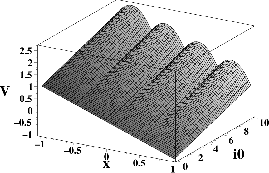
Figure 2: The washboard potential $V(x)$ defined by Eq. (10) for $p=1/2$ and temperature $T_{0}=0.5$. For the rescaled current amplitude $i_{0}>i_{c}$, the potential barriers appear. The critical value of the current amplitude $i_{c}$ is defined by the conditions $V^{\prime}(x)=0$ and $V^{\prime\prime}(x)=0$. For the presented set of parameters $i_{c}\approx 2$.

2 Flux-biased regime

We intend to investigate the flux-biased regime which is defined in the following way [7]: Let the external magnetic field $B$ increases giving rise to increase of the magnetic flux $\phi_{e}$. Let additionally the self-inductance $L$ increases. Formally, we perform the limit $\phi_{e}\to\infty$ and $L\to\infty$ in such a way that the ratio $\phi_{e}/L=I_{e}$ is fixed. In this limit, the generalized potential $W(\phi)$ approaches a washboard form. Indeed, in Fig. 1, we present four forms of the dimensionless generalized potential

$$W_{1}(x) \equiv \frac{W(\phi)}{\phi_{0}I_{0}}=\frac{1}{2L_{1}}\left(x^{2}-2x_{e}x\right)$$ (8)

$$+ \sum_{n=1}^{\infty}\frac{A_{n}(T/T^{*})}{2\pi n}\left\{p\cos\left(2\pi nx\right)+(1-p)\cos\left[2\pi n\left(x+1/2\right)\right]\right\},$$

with the dimensionless flux $x=\phi/\phi_{0}$, $x_{e}=\phi_{e}/\phi_{0}$ and the dimensionless inductance $L_{1}=LI_{0}/\phi_{0}$. We can notice that for the fixed ratio $x_{e}/L_{1}=\phi_{e}/(LI_{0})=I_{e}/I_{0}=1/5$ and for $x_{e}=20$ and $L_{1}=100$, the potential $W_{1}(x)$ is very well approximated by the biased washboard potential for large (but finite) number of periods of the coherent current $I_{coh}(\phi,T)$. In the flux-biased regime, the Langevin equation (5) takes the form

$$\frac{dx}{d\tau}=-\frac{dV(x)}{dx}+\sqrt{2D}\xi(\tau),$$ (9)

where the dimensionless time $\tau=t/\tau_{0}$ with $\tau_{0}=\phi_{0}/RI_{e}$ and the biased washboard potential $V(x)$ (see Fig. 2) reads

$$V(x) = V(x,T_{0})=\frac{L_{1}}{x_{e}}W_{1}(x)$$ (10)

$$= -x+i_{0}\sum_{n=1}^{\infty}\frac{A_{n}(T_{0})}{2\pi n}\left\{p\cos(2\pi nx)+(1-p)\cos\left[2\pi n(x+1/2)\right]\right\}$$

with the rescaled current amplitude $i_{0}=I_{0}/I_{e}$. The rescaled zero-mean Gaussian white noise $\xi(\tau)$ has the same $\delta$-auto-correlation function as $\Gamma(t)$. Its intensity $D=k_{0}T_{0}$, where the dimensionless temperature $T_{0}=T/T^{*}$ and $k_{0}=k_{B}T^{*}/\phi_{0}I_{e}$ is the ratio of thermal energy at the characteristic temperature $T^{*}$ to the energy of the flowing current $I_{e}$ induced by the elementary flux $\phi_{0}$.

The Langevin equation (9) can be interpreted in terms of the overdamped motion of the Brownian particle in the washboard potential (10). The periodic part of this potential is a ’ratchet type’ potential [8], i.e. $V(x)$ does not posses the reflection symmetry. Let us notice that for $p=1/2$, there is an additional periodicity $V^{\prime}(x+1/2)=V^{\prime}(x)$ presented in the system.

Figure 3: The averaged stationary flux velocity as a function of temperature $T_{0}$ for several (both subcritical and supercritical) values of $i_{0}$ and fixed $p=1/2$. Inset: The corresponding washboard potentials (10) at $T_{0}=1$ are depicted for $i_{0}=2$ (upper panel) and $i_{0}=10$ (lower panel).

Figure 4: The averaged stationary flux velocity as a function of $T_{0}$ for three values of $p$ and fixed $i_{0}=10$. Inset: The corresponding washboard potentials (10) at $T_{0}=1$ (upper panel) and $T_{0}=2$ (lower panel) are presented for three values of $p=0,0.25,0.5$.

3 Flux velocity

In this paper we shall study the averaged (with respect to the noise realizations) stationary flux velocity $\langle\dot{x}\rangle$ which is given by the formula [9]:

$$\langle\dot{x}\rangle=N\left[1-\exp\left(\frac{V(1,T_{0})-V(0,T_{0})}{D}\right)\right],$$ (11)

$$N^{-1}=D^{-1}\;\int_{0}^{1}dx\int_{x}^{x+1}dy\exp\left(\frac{V(y,T_{0})-V(x,T_{0})}{D}\right).$$ (12)

The flux velocity is a function of the system parameters. The first parameter is the temperature. The second one is the current amplitude $i_{0}$, which reflects the ability of accommodating persistent currents. The third one, $p\in[0,1]$, describes the structure of current channels as it is the probability of occurring current channel carrying even number of phase coherent electrons. Let us notice that, due to quantum size effects, persistent currents are always present in a sufficiently small system, i.e. there are always electrons maintaining their phase coherence when moving around the ring. The problem is if $i_{0}$ is sufficiently large for those electrons to produce significant contribution to the total current flowing in the system at a given temperature. Numerical results show that upon inspection of the properties of the flux velocity $\langle\dot{x}\rangle$ one can infer when the given ring is able to accommodate persistent current of a significant amplitude at a given temperature. In Fig. 4 we present the relation between the flux velocity and the temperature $T_{0}$ for several different values of the current amplitude $i_{0}$. The general tendency is that in the presence of persistent currents the flux velocity is suppressed at the low temperature $T_{0}$ or large $i_{0}$. There are two classes of the systems split by the critical value $i_{c}$ of the current amplitude $i_{0}$, which determines the inflection points of the potential. This qualitative change is defined by a set of two equations: $V^{\prime}(x)=0$ and $V^{\prime\prime}(x)=0$ and is presented in Fig 2. For $i_{0}>i_{c}$, barriers of the potential $V(x)$ exist. For $i_{0}<i_{c}$, the potential is a monotonic function of the flux $x$. Systems from the first class, with the supercritical amplitude $i_{0}>i_{c}$, exhibit vanishing flux velocity for $T_{0}\rightarrow 0$. For the second class systems, with the subcritical amplitude $i_{0}<i_{c}$, the flux velocity decreases but remains finite as temperature $T_{0}\to 0$. It is clear that in the formal limit $i_{0}=0$, the flux velocity is constant, $\langle\dot{x}\rangle_{|i_{0}=0}=1$. The critical value $i_{c}\approx 2$ is estimated for the ring with $p=1/2$.

In Fig. 4, the probability $p$ of a channel with an even number of coherent electrons is chosen as a parameter. For the system with statistically equal number of channels of both types ($p=1/2$), the flux velocity is greater than for systems with one type of channels dominating over the other (e.g. $p=0$). The results obtained for $p=1/4$ and $p=0$ coincide with $p=3/4$ and $p=1$ respectively and there is no way to distinguish with type of channels dominates in the ring.

In order to quantify the effect, one can define the ’susceptibility’, i.e. the temperature derivative of the averaged stationary flux velocity at fixed values of other parameters. Its monotonicity characterizes the possibility of obtaining persistent currents in the system. With this function one can associate a measure of the ability of accommodating persistent currents in the ring. This measure could be defined as a distance, in the sense of a metric in a function space, between the given (non-zero) susceptibility and the zero susceptibility.

In conclusion, we have shown that performing suitable limiting procedure one can obtain new significant informations about persistent currents in mesorings. Investigations of global properties of the flux velocity can serve as an additional characteristics of mesoscopic rings. The perfect example is the monotonicity of the temperature derivative of the flux velocity or its asymptotic behavior at low temperatures which carries information about possibility of appearing persistent currents in the ring.

References

-
[1]
Y. Makhlin, G. Schōn, A. Schnirman, Rev. Mod. Phys. 73,
357 (2001);
E. Zipper, M. Kurpas, M. Szela̧g, J. Dajka, M. Szopa, Phys. Rev. B74, 125426 (2006). -
[2]
F. Hund, Ann. Phys. (Leipzig) 32, 102 (1938);
I. O. Kulik, JETP Lett. 11, 275 (1970). -
[3]
L.P. Levy, G. Dolan, J. Dunsmouir, H. Bouchiat, Phys. Rev. Lett. 64, 2074 (1990);
U. Eckern, P. Schwab, J. Low Temp. Phys. 126, 1291 (2002). - [4] H.F. Cheung, Y. Gefen, E.K. Riedel, W.H. Shih, Phys. Rev. B 37, 6050 (1988).
- [5] J. Dajka, J. Łuczka, P. Hänggi, phys. stat. sol.b 242, 196 (2005).
-
[6]
J. Dajka, J. Łuczka, M. Szopa, E. Zipper, Phys. Rev. B67, 073305 (2003);
J. Dajka, M. Kostur, J. Łuczka, M. Szopa, E. Zipper, Acta Phys. Pol. B34, 3793 (2003). - [7] M.H. Devoret in Quantum fluctuations eds. S. Reynaud, E. Giacobino and J. Zinn-Justin, Les Houches LXIII (1995).
- [8] J. Łuczka, Physica A 274, 200 (1999).
- [9] J. Łuczka, R. Bartussek and P. Hänggi, Europhys. Lett. 31, 431 (1995).