Classical and quantum features of the superfluid to Mott insulator transition

Abstract

We analyze the correspondence of many-particle and mean-field dynamics for a Bose-Einstein condensate in an optical lattice. Representing many-particle quantum states by a classical phase space ensemble instead of one single mean-field trajectory and taking into account the quantization of the density by a modified integer Gross-Pitaevskii equation, it is possible to simulate the superfluid to Mott insulator transition and other phenomena purely classically. This approach can be easily extended to higher particle numbers and multidimensional lattices. Moreover it provides an excellent tool to classify true quantum features and to analyze the mean-field – many particle correspondence.

Introduction. Ultracold atoms in optical lattices provide an excellent model system for the study of fundamental condensed matter problems, since experimental parameters can be controlled in a wide range and with high accuracy. If the atomic interactions are weak, bosonic atoms form a Bose-Einstein condensate (BEC). In the superfluid phase all atoms occupy the same delocalized quantum state and can be described by a macroscopic wave function. The dynamics of the condensate wave function is given in a mean-field approach by the celebrated Gross-Pitaevskii equation (GPE). However, mean-field theory takes into account only expectation values and neglects quantum fluctuations. Hence it is widely believed to fail when fluctuations are of importance – striking examples are number squeezing and quantum phase transitions Orze01 ; Grei02 . In this Letter we propose a phase space ensemble approach based on the mean-field limit including quantum fluctuations. If the atomic interactions dominate the dynamics, the system undergoes a quantum phase transition from the superfluid (SF) to the Mott insulator (MI) phase even at zero temperature due to quantum fluctuations. Since its first experimental observation Grei02 this transition attracts more and more attention (see JaBl05 and references therein). The MI phase is charaterized by a finite gap in the excitation spectrum and a vanishing compressibility. Number fluctuations are frozen out and the long-range phase coherence is lost. In an overall confining potential this leads to the appearance of a distinct shell structure. This pinning of the on-site occupation number to integer values has only recently been observed experimentally Foel06 .

If the optical lattice is sufficiently deep, the dynamics of the atoms is described by the Bose-Hubbard model Hamiltonian Fish89b

$$\hat{H}=\sum\nolimits_{j}\left(-J(\hat{a}_{j+1}^{\dagger}\hat{a}_{j}+\hat{a}_{j}^{\dagger}\hat{a}_{j+1})+\epsilon_{j}\hat{n}_{j}+\frac{U}{2}\hat{n}_{j}^{2}\right),$$ (1)

where $\hat{a}_{j}$ is the bosonic annihilation operator at the $j$-th lattice site and $\hat{n}_{j}=\hat{a}_{j}^{\dagger}\hat{a}_{j}$. As the Bose-Hubbard model is a genuine many-particle problem, approximations are of exorbitant interest. Numerically exact calculations can only be done for very few particles since the Hilbert space of the many-particle quantum states grows exponentially both with the particle number and the size of the lattice.

The mean-field approximation for a weakly interacting Bose gas is usually derived within a Bogoliubov approach, considering the expectation values $\langle\hat{a}_{j}\rangle=\sqrt{N}\psi_{j}$ only. Starting from the Heisenberg equations of motion for the operators $\hat{a}_{j}$ and neglecting quantum fluctuations $\langle\hat{a}_{j}^{\dagger}\hat{a}_{j}^{2}\rangle\approx\langle\hat{a}_{j}^{\dagger}\rangle\langle\hat{a}_{j}\rangle^{2}$ yields the discrete GPE

$$i\dot{\psi}_{j}=-J(\psi_{j+1}+\psi_{j-1})+UN|\psi_{j}|^{2}\psi_{j}$$ (2)

for the classical field $\psi_{j}$. This ansatz is exact for vanishing interaction $U=0$ and can be compared to the Ehrenfest theorem in single particle quantum mechanics.

In this Letter we will propose a phase space approach to the mean-field limit and a generalization of the GPE which enables us to describe squeezed states and the SF-MI-transition purely classically. In contrast to the established Bogoliubov approach the many-particle state is represented by an ensemble of mean-field trajectories, taking into account also the higher moments of the many particle quantum state. The quantization of the density $\hat{n}_{j}$ which gives rise to the Mott shell structure is achieved by the introduction of an integer Gross-Pitaevskii equation (IGPE). The phase space IGPE dynamics can be easily implemented and efficiently simulated even for higher particle numbers and two- or three-dimensional lattices. Moreover we will show that it provides an excellent tool to classify true quantum features and analyze the mean-field – many-particle correspondence like the break down of the mean-field approximation at unstable classical fixed points CaVa97 .

Quantum phase space. The key idea of the phase space IGPE approach is to map the quantum many-particle state onto an ensemble of trajectories in classical phase space, whose dynamics is given by the IGPE. Instead of quantum expectation values we will consider time-dependent classical ensemble averages. The initial ensemble is distributed according to a quantum quasi-probability distribution to transfer the characteristics of the quantum state onto the classical phase space. The Husimi distribution provides a non-negative and bounded function on quantum phase space, which is hence particularly suited for a comparison to the classical phase space distribution. Any many-particle quantum state $\left|\Psi\right\rangle$ can be represented by the Husimi distribution, which is given by the projection onto coherent states $\left|\{c_{j}\}\right\rangle$,

$$Q_{\left|\Psi\right\rangle}(c_{1},\ldots,c_{M})=\left|\langle\{c_{j}\}|\Psi\rangle\right|^{2}.$$ (3)

In general, the structure of quantum phase space is determined by the operator algebra generated by the commutation relations of $\hat{a}_{j}$ and $\hat{a}_{j}^{\dagger}$. For the $M$-site Bose-Hubbard model, the relevant algebra is SU($M$), which reflects the conservation of the number of particles. The generalized coherent states Pere86

$$\left|\{c_{j}\}\right\rangle=\frac{1}{\sqrt{N!}}\bigg{(}\sum\nolimits_{j=1}^{M}c_{j}\hat{a}_{j}^{\dagger}\bigg{)}^{N}\left|0\right\rangle$$ (4)

are parametrized by the amplitudes at the lattice sites $c_{j}$ which are normalized as $\sum\nolimits_{j}|c_{j}|^{2}=1$. These concepts are most easily understood for the special case of just two lattice sites, where one can introduce the operators $\hat{L}_{x}=\frac{1}{2}(\hat{a}_{1}^{\dagger}\hat{a}_{2}+\hat{a}_{2}^{\dagger}\hat{a}_{1}),\;\hat{L}_{y}=\frac{i}{2}(\hat{a}_{2}^{\dagger}\hat{a}_{1}-\hat{a}_{1}^{\dagger}\hat{a}_{2})$ and $\hat{L}_{z}=\frac{1}{2}(\hat{a}_{1}^{\dagger}\hat{a}_{1}-\hat{a}_{2}^{\dagger}\hat{a}_{2}),$ which form an angular momentum algebra SU(2) with quantum number $\ell=N/2$ MiSm97 . The Hamiltonian (1) then can be rewritten in the Bloch representation as $\hat{H}=-2J\hat{L}_{x}+U\hat{L}_{z}^{2}$ up to a constant term. Since the SU(2)-algebra is topological equivalent to the (Bloch-)sphere $S^{2}(\theta,\phi)$, the coherent states and the Husimi distribution can be parametrized by the polar angle $\theta$ and the azimuth angle $\phi$ via the identification $c_{1}=\sqrt{(1+\cos\theta)/2}$ and $c_{2}={\rm e}^{i\phi}\sqrt{(1-\cos\theta)/2}$. The dynamics of the Husimi distribution $Q$ is then given by Trim07

$$\dot{Q} = UN\left(\cos(\theta)-\frac{1}{N}\sin(\theta)\frac{\partial}{\partial\theta}\right)\frac{\partial}{\partial\phi}Q$$ (5)

$$-J\left(\sin(\phi)\frac{\partial}{\partial\theta}+\cos(\phi)\frac{\cos\theta}{\sin\theta}\frac{\partial}{\partial\phi}\right)Q.$$

The integer GPE. The classical Hamiltonian function ${\cal H}$ of the mean-field dynamics, $id\psi_{j}/dt=\partial{\cal H}/\partial\psi_{j}^{*}$, is given by the expectation value of the many-particle Hamiltonian (1), again neglecting quantum fluctuations:

$${\cal H}=\sum\nolimits_{j}\left(-J(\psi_{j+1}^{*}\psi_{j}+c.c.)+\epsilon_{j}|\psi_{j}|^{2}+\frac{UN}{2}|\psi_{j}|^{4}\right).$$ (6)

However, the quantum fluctuations, in particular the variance of the density, are of fundamental importance in the MI phase. In principle these fluctuations act like an effective macroscopic variable driving the system towards integer filling. This can be already understood in the case of two wells: One can show that in the limit of strong number squeezing the quantum term $\sim\partial^{2}Q/\partial\theta\partial\phi$ in Eq. (5) simplifies and the dynamics becomes exactly Liouvillian again Trim07 , however with a modified Hamiltonian function including a term describing quantum pressure. Generalizing this exact result to an extended lattice we propose a modification of the GPE including the additional energy $\Delta{\cal H}=U/2\sum\nolimits_{j}(\langle\hat{n}_{j}^{2}\rangle-\langle n_{j}\rangle^{2})$ due to the quantization of the number operator. This term is only relevant if the interaction energy dominates the dynamics. In this case the lattice wells decouple and the many-particle wave function is given by the Gutzwiller ansatz as a direct product $\left|\Psi\right\rangle=\left|\Psi_{1}\right\rangle\otimes\cdots\otimes\left|\Psi_{M}\right\rangle$, where the local wave functions are written in a Fock basis $\left|\Psi_{j}\right\rangle=\sum\nolimits_{n_{j}}b_{n_{j}}\left|n_{j}\right\rangle$. Assuming that the local density is given by the mean-field expectation value $N|\psi_{j}|^{2}$, the minimal ansatz for the local quantum state reproducing this density is given by

$$\left|\Psi_{j}\right\rangle=\sqrt{1-d_{j}}\left|m_{j}\right\rangle+\sqrt{d_{j}}e^{i\beta}\left|m_{j}+1\right\rangle,$$ (7)

where $m_{j}$ is the integer part of the local density, i.e. $N|\psi_{j}|^{2}=m_{j}+d_{j}$ with $m_{j}\in\mathbb{N}$. The variance of the density is then given by $\langle\hat{n}_{j}^{2}\rangle-\langle n_{j}\rangle^{2}=d_{j}-d_{j}^{2}$. This ansatz presumes the smallest possible variance and thus the minimal energy correction $\Delta{\cal H}$ with respect to the GPE Hamiltonian (6). Including this correction, Hamilton’s equations yield an integer Gross-Pitaevskii equation (IGPE)

$$i\dot{\psi}_{j}=-J(\psi_{j+1}+\psi_{j-1})+\epsilon_{j}\psi_{j}+U(m_{j}+1/2)\psi_{j}.$$ (8)

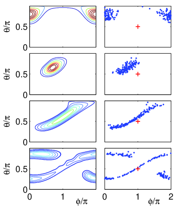
Figure 1: (Color online) Comparison of quantum and classical dynamics in phase space approaching the hyperbolic fixed point for $UN=10$, $J=1$ and $N=20$ particles. Left: Evolution of the Husimi density. Right: Dynamics of an ensemble of 150 classical trajectories at times $t=0,0.3,0.6,0.9$.

Bogoliubov vs. phase space approach. As a first illustrative example, we consider the dynamics of the two-mode system. In the mean-field limit, the quantum expectation value $\langle\hat{\mathbf{L}}\rangle/N$ is approximated by the Bloch vector

$$\mathbf{s}=\frac{1}{2}\left(\begin{array}[]{c}\psi_{1}^{*}\psi_{2}+\psi_{2}^{*}\psi_{1}\\ i(\psi_{2}^{*}\psi_{1}-\psi_{1}^{*}\psi_{2})\\ |\psi_{1}|^{2}-|\psi_{2}|^{2}\end{array}\right).$$ (9)

The dynamics of $\mathbf{s}$ is restricted to the (Bloch-)sphere, reflecting the conservation of normalization. In the non-interacting case $UN=0$ the system performs common Rabi oscillations between the two modes. The anti-symmetric fixed point bifurcates for $UN>2J$, forming two novel elliptic and one hyperbolic fixed point. The two novel fixed points have a non-vanishing population difference $s_{z}\neq 0$, leading to the ‘self-trapping’ effect MiSm97 .

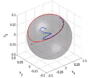
Figure 2: (Color online) Comparison of the many-particle expectation value $\langle\mathbf{L}(t)\rangle/N$ (blue line), the Bogoliubov approximation $\mathbf{s}(t)$ (red line) and the ensemble average $\langle\mathbf{s}(t)\rangle_{\rm cl}$ for 1000 classical trajectories (dashed green line). Parameters are chosen as in Fig. 1.

At the hyperbolic fixed point the classical dynamics becomes unstable and the Bogoliubov approach breaks down CaVa97 . This is mirrored in quantum phase space as shown in Fig. 1: The initial coherent state at $\theta=0.8\pi$ and $\phi=0$ diffuses in the direction of the unstable manifold. Therefore the quantum expectation value $\langle\hat{\mathbf{L}}(t)\rangle/N$ penetrates into the Bloch sphere in the vicinity of the hyperbolic fixed point (marked by $+$ in Fig. 2), whereas the single classical trajectory $\mathbf{s}(t)$ stays on the Bloch sphere. However, this is by no means a breakdown of the mean-field approximation in phase space. As demonstrated in Fig. 1 the dynamics of a classical ensemble closely follows the dynamics of the Husimi distribution. The dynamics of the quantum expectation value $\langle\hat{\mathbf{L}}\rangle/N$ is well reproduced by the ensemble average $\langle\mathbf{s}\rangle_{\rm cl}$ as shown in Fig. 2.

The phase space approach can describe certain features of the quantum dynamics, such as squeezing and the dynamics at the unstable classical fixed point. Other aspects of the dynamics are genuine quantum like interference and tunneling in phase space. On the opposite, the GPE exactly reproduces the dynamics of the expectation value $\langle\hat{\mathbf{L}}\rangle$ for $U=0$. However, the system is not necessarily ‘classical’ (cf. Ball94 ).

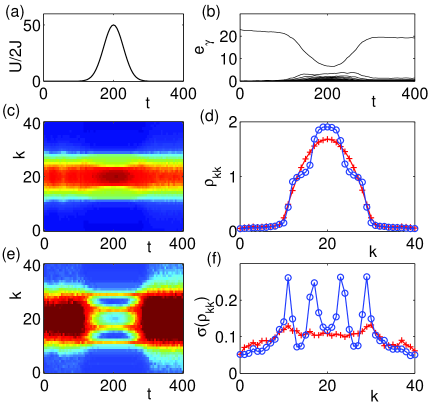
Figure 3: (Color online) Dynamics of the SF-MI transition in a harmonic trap with $\omega=0.17$, $M=40$ and $N=26$ particles calculated from classical ensemble averages: Variation of the parameters (a), eigenvalues of the classical SPDM (b), density $\rho_{kk}$ (c-d) and its standard deviation $\sigma(\rho_{kk})$(e-f). Figures (d) and (f) show $\rho_{kk}$ and $\sigma(\rho_{kk})$ in the Mott phase at time $t=t_{c}$ calculated with the IGPE (blue circles) and the usual GPE (red crosses).

The superfluid to Mott insulator transition. The SF-MI transition is considered to be not explicable within mean-field theory because it is driven by quantum fluctuations. However, the phase space IGPE method takes into account fluctuations as well as the quantization of the density $\hat{n}_{j}$. Therefore it provides a fully classical description of the the SF-MI transition. We consider the dynamics of $N=26$ particles in an optical lattice with a superimposed harmonic trap described by the Bose-Hubbard Hamiltonian (1) with $\epsilon_{k}=\omega^{2}(k-k_{0})^{2}/2$. We assume that the lattice is initially loaded with a pure BEC in the Gross-Pitaevskii ground state $\psi_{j}$. The depth of the lattice is then increased adiabatically, suppressing the tunneling between the lattice sites, and decreased back again. This is described by a time-dependent hopping matrix element $J(t)=J_{0}[1+A{\rm e}^{-(t-t_{c})^{2}/t_{s}^{2}}]^{-1}$ with $J_{0}=20$, $A=10^{3}$, $t_{c}=200$ and $t_{s}=40$, while the interaction strength $U=1$ is kept constant. We calculate the time evolution of an ensemble of 200 mean-field trajectories, whose initial amplitudes $c_{k}(t=0)$ are distributed according to the Husimi function (3). A classical approximation of the single-particle density matrix (SPDM) $\rho_{kl}=\langle\hat{a}_{k}^{\dagger}\hat{a}_{l}\rangle$ is then provided by the ensemble average $\rho_{kl}=\langle c_{k}^{*}c_{l}\rangle_{\rm cl}$. Figure 3 shows some characteristic features of the MI-SF transition calculated with the phase space IGPE, reproducing the results obtained by full many-body calculations Clar04 ; Koll04 . Indeed one observes the occurrence of Mott shells with integer filling, $\rho_{kk}\in\mathbb{N}$, and small superfluid regions in between. The density fluctuations are strongly suppressed in the MI phase, whereas they are significantly stronger between the Mott shells. In the SF phase one eigenvalue of the SPDM is close to the particle number, indicating that the many-particle state is a coherent state described by one single condensate wave function $\psi_{j}$. In contrast, the MI phase is characterized by many eigenvalues of the same magnitude. This state cannot be described by a single condensate wave function, but by a phase space distribution. Figure 4 shows the magnitude of the SPDM itself. One clearly sees that the coherences are lost in the MI phase at $t=t_{c}$ and mostly restored at $t=2t_{c}$. The SF-MI transition is reversible to a large extent, which is demonstrated by increasing $J(t)$ again for $t>t_{c}$.

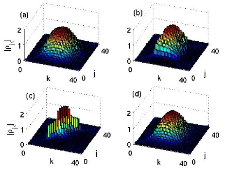
Figure 4: (Color online) Dynamics of the SF-MI transition in a harmonic trap: Magnitude of the classical SPDM $|\rho_{kl}|$ at $t=0,130,200,400$ (a-d).

Let us notice that the suppression of density fluctuations and the loss and revival of coherences is already introduced into mean-field theory by the phase space ensemble approach. However, the usual GPE cannot reproduce the Mott shells and the energy gap of the particle-hole excitations, because the quantization of the density is neglected. This becomes most obvious in Fig. 3 (d) and (f). The GPE predicts a smooth Thomas-Fermi density profile and a uniform suppression of density fluctuations in the MI phase.

The occurrence of a gap in the excitation spectrum in the MI phase can also be understood within the classical phase space approach. Low-energy phonons cannot be excited as such collective excitations are impossible if the spatial coherences are lost. The remaining excitations in the MI phase are density fluctuations, which are discrete in the IGPE description.

Conclusion and outlook. Summarizing, we map the many particle quantum state to a phase space ensemble obeying a modified GPE including the backreaction of the quantum fluctuations onto the order parameter. The example of the SF-MI phase transition proves the power of the phase space ensemble method, providing an enormous alleviation of numerical effort and an illustrative insight into the many-particle dynamics. For example, the depletion of a BEC at a classically unstable point CaVa97 can be fully understood using phase space ensembles. The atoms are not lost – they are just redistributed to other modes. The phase space interpretation gives rise to fundamental questions: Which properties of a BEC are essentially quantum? Further work will be devoted to extended three-dimensional lattices and to a deeper analysis of the classical limit of many-particle quantum dynamics. Which criteria determine whether a many-particle system can be simulated classically? Advanced algorithms for many-particle simulations exploit the weak entanglement in 1D quantum systems Vida04 and not the classicality of the state.

Support from the Studienstiftung des deutschen Volkes and the DFG (GRK 792) is gratefully acknowledged. We thank M. Fleischhauer and J. R. Anglin for stimulating discussions.

References

- (1) C. Orzel, A. K . Tuchman, M. L. Fenselau, M. Yasuda, and M. A. Kasevich, Science 291, 2386 (2001)
- (2) M. Greiner, O. Mandel, T. Esslinger, T. W. Hänsch, and I. Bloch, Nature 415, 39 (2002)
- (3) D. Jaksch and P. Zoller, Ann. Phys. (N.Y.) 315, 52 (2005); I. Bloch, Nature Phys. 1, 23 (2005).
- (4) S. Fölling, A. Widera, T. Müller, F. Gerbier, and I. Bloch, Phys. Rev. Lett. 97, 060403 (2006); G. Campbell et al., e-print cond-mat/0606642
- (5) M. P. A. Fisher, P. B. Weichman, G. Grinstein, and D. S. Fisher, Phys. Rev. B 40, 546 (1989); D. Jaksch, C. Bruder, J. I. Cirac, C. W. Gardiner, and P. Zoller, Phys. Rev. Lett. 81, 3108 (1998)
- (6) Y. Castin and R. Dum, Phys. Rev. Lett. 79, 3553 (1997); A. Vardi and J. R. Anglin, Phys. Rev. Lett. 86, 568 (2001); J. R. Anglin and A. Vardi, Phys. Rev. A 64, 013605 (2001)
- (7) A. M. Perelomov, Generalized Coherent States and Their Applications, Springer, Berlin Heidelberg New York, 1986
- (8) G. J. Milburn, J. Corney, E. M. Wright, and D. F. Walls, Phys. Rev. A 55, 4318 (1997); A. Smerzi, S. Fantoni, S. Giovanazzi, and S. R. Shenoy, Phys. Rev. Lett. 79, 4950 (1997)
- (9) F. Trimborn, D. Witthaut, and H. J. Korsch, in preparation
- (10) L. E. Ballentine, Y. Yang and J. P. Zibin, Phys. Rev. A 50, 2854 (1994)
- (11) S. R. Clark and D. Jaksch, Phys. Rev. A 70, 043612 (2004); New J. Phys. 8, 160 (2006)
- (12) C. Kollath, U. Schollwock, J. vonDelft, and W. Zwerger, Phys. Rev. A 69, 031601(R) (2004); P. Sengupta, M. Rigol, G. G. Batrouni, P. J. H. Denteneer, and R. T. Scalettar, Phys. Rev. Lett. 95, 220402 (2005)
- (13) G. Vidal, Phys. Rev. Lett. 93, 040502 (2004)