Electron-phonon interaction in Graphite Intercalation Compounds

Abstract

Motivated by the recent discovery of superconductivity in Ca- and Yb-intercalated graphite (CaC₆ and YbC₆) and from the ongoing debate on the nature and role of the interlayer state in this class of compounds, in this work we critically study the electron-phonon properties of a simple model based on primitive graphite. We show that this model captures an essential feature of the electron-phonon properties of the Graphite Intercalation Compounds (GICs), namely, the existence of a strong dormant electron-phonon interaction between interlayer and $\pi^{\ast}$ electrons, for which we provide a simple geometrical explanation in terms of NMTO Wannier-like functions. Our findings correct the oversimplified view that nearly-free-electron states cannot interact with the surrounding lattice, and explain the empirical correlation between the filling of the interlayer band and the occurrence of superconductivity in Graphite-Intercalation Compounds.

Introduction

Superconductivity in Ca- and Yb-intercalated graphite (CaC₆ and YbC₆), with $T_{c}$ of respectively 11.5 and 6.5 K, was discovered YbC6:weller:syn ; CaC6:emery:syn five years later than in the pseudo-graphite MgB${}_{2},$ where $T_{c}$=40 K. MgB2_expt1 Superconductivity in MgB₂ is understood to be caused by the strong interaction between a few zone-centered holes in the B$\,sp^{2}$ $\sigma$-bonding band and a few zone-centered bond-stretching phonons, which themselves get softened by the interaction;MgB2_theory ; Pickett ; Kong ; BoeriDiamond the $\pi$ bands are also at the Fermi level, but they couple to phonons only weakly. What makes MgB₂ special is that the electrostatic and covalent attraction of the B $p_{z}\,\pi$ electrons by the intercalated Mg⁺⁺ ions is so strong that the center of the $\pi$ bands is lowered below the top of the $\sigma$ band, whereby hole-doping takes place into this bonding band. An equally simple and elegant understanding of the origin of superconductivity in the strongly electron-doped CaC₆ and YbC₆ is still missing. Csanyi et al. GIC:csanyi:band have empirically related the appearance of superconductivity in Graphite-Intercalation Compounds (GICs) to the filling of a free-electron-like interlayer (IL) band, GIC:posternak:band ; GIC:fauster:band which is present, albeit empty, in pure graphite; and proposed that plasmon-mediated superconductivity could take place in these compounds.Recent experiments CaC6:jskim:Cp ; CaC6:lamura:penetration and ab-initio calculations GIC:mazin:band ; CaC6:calandra:band ; CaC6:jskim:press ; RMTACaC6_pressure agree, instead, that the conventional e-ph coupling suffices to explain the superconductivity in CaC₆ and YbC₆, although some puzzling issues remain.GICs:Mazin:review

It seems therefore that in graphite, if the Fermi surface has only $\pi$ sheets, the e-ph coupling is weak and $T_{c}\lesssim 1\,$K, whereas, if also $\sigma$ or IL sheets are present, the e-ph coupling increases enough as to yield much higher $T_{c}$’s. Mazin et al. GIC:mazin:band and Calandra et al. CaC6:calandra:band argued that the main role in the e-ph coupling is played by electronic and vibrational states associated with the presence of the intercalant ion, and, generally speaking, this is true: without the intercalant, graphite is not a superconductor. However, a close inspection of the e-ph spectral functions $\alpha^{2}F(\omega)$ of CaC₆ of Refs. CaC6:calandra:band, ; CaC6:jskim:press, shows that a considerable fraction ($60\%$) of the total e-ph coupling comes from modes which involve carbon atoms and not the intercalant ion. This observation, together with the empirical correlation between the filling of the IL band and superconductivity, suggests that, in analogy with the hole-doped graphite compound MgB₂, CaC₆ and YbC₆ might be understood as “electron-doped graphite”, where a different source of e-ph interaction is switched on when electrons are driven into the IL band.

In this paper we will show, via density-functional-theory calculations,DFT that indeed a strong interband e-ph interaction between $\pi^{*}$ and IL electrons, due to out-of-plane phonons, survives in graphite even when the intercalant atom is replaced by a uniform positive background of charge (Jellium-Intercalated-Graphite, JIG).GIC:csanyi:band Such a finding contrasts with the rough idea that the IL states, being free-electron like, cannot interact with the surrounding lattice: this may become true when the carbon layers are very far apart from each other, but not at the spacings observed in real GICs, where, as our results clearly show, the IL states are strongly affected both by the presence and by the dynamics of the carbon layers which sandwich them. Similar confined, free-electron states are found in several layered materialsboride:medvedeva:band ; CaAlSi:gianto:band ; LiB:curtarolo:band ; LiB:mazin:band and even in nanotubes, NFES_in_CNTs where our results suggest that similar e-ph coupling interactions may take place.

The paper is organized as follows: in the first section we discuss the electronic structure of JIG with the aid of Wannier functions. In the second and third sections we calculate the vibrational spectrum and e-ph interaction of JIG. We then consider these as a function of doping and interlayer spacing in the fourth section, comparing the results of our model with the available experimental data on GICs. Finally, in Appendix A, we provide a minimal $3\mathrm{\times}3$ tight-binding model for JIG, while Appendix B contains the computational details for the different methods used: planewaves and pseudopotentials, PWscf TB-LMTO Theory:andersen:TBLMTOASA and NMTO. Theory:andersen:NMTO

I Electrons

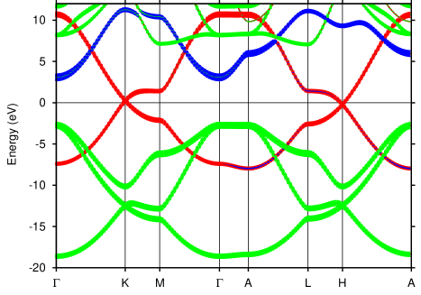
Figure 1: (Color Online) Band structure of primitive graphite. The fatness (and color) of the bands is proportional to the partial contribution of each orbital channel: green ($\sigma$), red ($\pi$) and blue (interlayer $\equiv$ IL). fatbandcharacter The lattice constants used in this plot are those of CaC₆ (see text and note CaC6structure, ). The Fermi level of CaC₆ would in this simple picture be at about 4.5 eV, see also Fig. 9.

A good starting point to understand the more complicated band structure of actual GICs, such as CaC₆ and YbC₆, is represented by primitive graphite. In this structure (space group 191) the carbon hexagons sit on top of each other ($\alpha\alpha\alpha$ stacking), i.e., they are not laterally shifted like in real graphite; the primitive cell thus contains two carbon atoms (C₂).

The color and fatness fatbandcharacter of the electronic bands of C₂, shown in Fig. 1, indicate the relative importance of the partial contribution of each orbital channel to the given band: green ($\sigma$), red ($\pi$), and blue (IL).

With $\alpha\alpha\alpha$ stacking and negligible dispersion perpendicular to the sheets, the bonding $\pi$ and antibonding $\pi^{\ast}$ bands touch at a (Dirac) cone in energy-versus-momentum space; with an occupancy of 4 electrons per C, the Fermi surface consists of merely the K-points in the Brillouin zone; simple graphite is an ideal semimetal. In the simplest rigid-band picture, hole-doping shifts the Fermi level down, towards and eventually inside the $\sigma$ bands, like in MgB${}_{2}.$ Electron-doping shifts the Fermi level up, and eventually brings it into the IL band (CaC₆, YbC₆, and other GICs).

The main difference between the rigid-band picture and actual GICs is that the intercalation of positive ions between the graphene layers shifts the IL bands down in energy with respect to the $\pi$ bands, without substantially modifying their shape in the relevant energy window;GIC:csanyi:band ; GICs:Mazin:review this effect is reproduced quite well even if one replaces the intercalant ions by a uniform background of positive charge (JIG), provided that the interlayer spacing is fixed at the corresponding value of the actual GIC.GIC:csanyi:band

While the nature of the $\sigma$ and $\pi$ bands has been extensively discussed in literature, less information is available about the IL band in GICs. IL states have mainly been described as three-dimensional, nearly-free electrons in the empty interlayer region, whence their name; and indeed, as far as the motion parallel to the graphite planes is concerned (the $xy$ directions), the IL electrons, to a very good approximation, freely propagate in the interstitial volume, with plane-wave-like wavefunction ${\rm exp}(ik_{x}x+ik_{y}y)$ and energy dispersion $\frac{1}{2}(k_{x}^{2}+k_{y}^{2})$.

In the $z$ direction, however, their motion is not free, being periodically damped, with period $c$, by the graphene layers, across which the IL electrons are only partially transmitted. Along $z$, these layers act like the periodic potential barriers of the Kronig-Penney model, Kittel where the free-electron parabola $\frac{1}{2}k_{z}^{2}$ is split into a set of sub-bands separated by gaps, with sub-bandwidths and gaps dictated by the strength of barriers and by their spatial separation $c$. In this model all gaps close, and the full 3D free-electron dispersion is recovered, for vanishing barrier strength; at fixed $c$, as the barrier strength increases, the transmission across potential barriers decreases, until, for infinite strength, electrons are confined between pairs of barriers, yielding a set of completely flat sub-bands; in our case this translates into IL bands $\varepsilon_{m}=\frac{1}{2}(k_{x}^{2}+k_{y}^{2})+\frac{1}{2}(m\pi/c)^{2},m=1,2,...$ with no dispersion along $k_{z}$.

A careful examination of different GICs (and of C₂ for several values of $c/a$) confirms that their IL bands stay somewhere between these two limiting cases, with the graphene layers approximately behaving, along $z$, as an array of barriers with fixed finite strength and variable period $c$, which depends on the intercalant atom. These bands have a substantial dispersion along $k_{z}$ –so there is significant transmission across the graphene layers, or, in other words, the IL electrons are not completely confined; but their slope and width strongly depend on $c$ –so the partial reflection against the graphene layers is significant too.

In the range of parameters analyzed in the present paper, which correspond to existing donor-intercalated graphites, the lowest $m=1$ Kronig-Penney band is well separated in energy from the others –another evidence that, in the $z$ direction, the nearly-free-electron theory does not hold for the IL states– and it is the only one which can be occupied; to this band we refer, in the following, as the IL band (blue in Fig. 1).

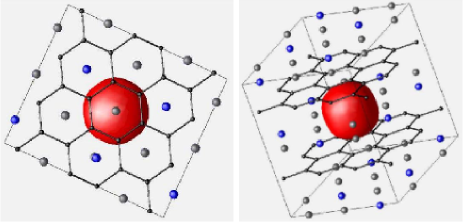
Figure 2: (Color Online) Top and side view of the Wannier-like NMTOAppA function $\psi_{s}(\mathbf{r})$, see also Appendix A, for the IL band (blue in Fig.1). The basis set spanning the IL band consists of the replicas of this function placed at all interstitial sites (grey and blue spheres). The figure shows the contour $\left|\psi_{s}(\mathbf{r})\right|=0.07\times(a.u.)^{-3}$, with $\int\psi_{s}^{2}d^{3}r=1.$ The sign of $\psi_{s}(\mathbf{r})$ is indicated by red and green.

In Fig. 2 we show the shape of its Wannier functionNMTOnote . Because the IL band overlaps other bands –the $\pi^{\ast}$ and $\sigma^{\ast}$ bands, with which it, however, hybridizes very little,– and because the function shown in Fig. 2 has not yet been symmetrically orthogonalized to the lattice-translated functions, it ought to be called Wannier-like as in Refs. Theory:andersen:NMTO, and ZurekNMTO, . The basis set spanning the IL band, interpolated smoothly across any hybridization gap, consists of this Wannier-like function and its replicas displaced by all lattice translations. We have chosen the IL Wannier-like function to be centered on an interstitial site, where it is seen to have the full point-group symmetry and a simple, $s$-like shape. The bond-centered Wannier-like function for the $\pi^{\ast}$ band,ZurekNMTO interpolated smoothly across hybridization gaps, is the antibonding linear combination of the two C$\,p_{z}$ orbitals at the vertices of the bond, plus a halo of further antibonding $C$ $p_{z}$ orbitals. The basis set spanning the $\pi^{\ast}$ band consists of this Wannier-like function and its replicas displaced by all lattice translations. That is, every second C-C bond carries such a function. Since the IL Wannier-like function has everywhere the same sign, while the sign of the $\pi^{\ast}$ Wannier-like function alternates within the scale of the IL function (there is one IL function for every two C $p_{z}$ orbitals), the two functions, one displaced against the other by an arbitrary lattice translation, are very nearly orthogonal. This is the reason why the IL and $\pi^{\ast}$ bands hardly hybridize, as seen in Fig. 1. On the contrary, the Wannier-like function for the $\pi$ bandZurekNMTO is the bonding linear combination of the two C$\,p_{z}$ orbitals at the vertices of the bond, and that is not orthogonal to the IL function. For that reason, the $\pi$ band may hybridize with the IL band, as will be discussed in Appendix A. This hybridization shows up if, by doping or changes in the $c/a$ ratio, the IL band moves into the energy region of the $\pi$ band.

Based on the band and orbital picture of primitive graphite (C₂) discussed so far, in the following sections we will study the electron-phonon properties of JIG, i.e. an artificially electron-doped C₂, where the electrons in excess are neutralized by a uniform, positive background charge; the comparison of the band structure of JIG with that of real GICs has shown that two important independent variables govern the filling of the interlayer band: the interlayer spacing $c$ and the number of electrons added to the system. In our study, these two parameters are represented by the doping $n$, defined as the number of electrons added to C${}_{2},$ and neutralized by a jellium background of the same magnitude (the number of C valence electrons is thus $4+n/2$) and the $c/a$ ratio of a C₂ unit cell with the same in-plane lattice constant as CaC₆. To minimize the number of parameters we in fact kept the in-plane lattice constant fixed throughout our study, so varing $c$ is like varying $c/a$.

II Phonons

The top left part of Fig. 3 shows the phonon dispersions we calculated for the doping levels $n\mathrm{=}0$ (dotted, pure graphite) and $n\mathrm{=}2/3$ (corresponding to CaC₆, full line). We used the interlayer spacing $c$ and planar lattice constant $a$ of CaC₆ in both cases, to compare with available experimental and theoretical data. With two atoms per cell there are 6 phonon branches, and since a phonon displacement is a vector like an electronic C$\,p$ function, the 6 phonon branches are topologically equivalent with the electronic C $\,p$ bands, that is, with the $\pi$ and $\pi^{\ast}$ bands and with the non-$s$ part of the $\sigma$ and $\sigma^{\ast}$ bands in Fig. 1. In particular, the two phonon branches which are the softest along KH, are the out-of-plane vibrations with dispersions similar to those of the $\pi$ bands in Fig. 1; the four other branches are the in-plane vibrations. In-plane and out-of-plane modes hardly mix. For that reason, the $n\mathrm{=}0$ and $n\mathrm{=}2/3$ phonon dispersions are qualitatively similar.

The only qualitative difference occurs along the $\Gamma$-A-L path, where the out-of-plane acoustic branch of JIG has imaginary frequencies. Such an instability is an artifact of JIG: at $n=0$ this branch is just very soft and sensitive to computational details, but not unstable;graf:marzari:band in actual GICS the intercalants contribute to the inter-layer binding and stabilize the strucure. Fortunately this artificial JIG instability occurs where the e-ph interaction is unimportant (no green dots where the frequencies are negative in the upper left panel of Fig. 3), and does not affect our subsequent analysis.

In real CaC₆ and other GICs GIC:calandra:band in- and out-of-plane C modes are also separated in energy, and occur at similar energy scales, and they do not mix with the intercalant modes, which are at a lower energy scale ($\omega\sim 10$ meV in CaC₆ CaC6:calandra:band ; CaC6:jskim:press ).

III Electron-Phonon coupling

III.1 Jellium Intercalated Graphite (JIG)

In a metal, e.g. for doped graphite, the $\nu\mathbf{q}$ phonon can couple between electrons $n\mathbf{k}$ and $m\left(\mathbf{k+q}\right)$ at the Fermi surface, and thereby attain a relative line-width:

$$\frac{\gamma_{\nu\mathbf{q}}}{\omega_{\nu\mathbf{q}}}=2\pi\sum_{nm\mathbf{k}}|g_{\nu,\,n\mathbf{k},\,m\left(\mathbf{k+q}\right)}|^{2}\delta(\varepsilon_{n\mathbf{k}})\delta(\varepsilon_{m\mathbf{k+q}}).$$ (1)

Here, $\sum_{\mathbf{k}}$ is the average over the Brillouin zone and

$$g_{\nu,n\mathbf{k},m\left(\mathbf{k+q}\right)}=\left\langle n\mathbf{k}\left|\delta V\left(\mathbf{r}\right)\right|m\left(\mathbf{k+q}\right)\right\rangle/\delta Q_{\nu\mathbf{q}}$$ (2)

is the matrix element of the perturbation, $\delta V\left(\mathbf{r}\right),$ of the self-consistent electronic potential due to the displacement,

$$\delta R_{\alpha j}=\frac{e_{\alpha j,\nu\mathbf{q}}}{\sqrt{2M_{j}\omega_{\nu\mathbf{q}}}}\delta Q_{\nu\mathbf{q}},$$

in the $\alpha$-direction of the $j$th atom (and continued as a wave with wavevector $\mathbf{q),}$ $e_{\alpha j,\nu\mathbf{q}}$ being the eigenvector of the $\nu\mathbf{q}$ phonon.

The squared e-ph matrix element is usually a smoother function of $\mathbf{k}$ and $\mathbf{k+q}$ than $\delta(\varepsilon_{n\mathbf{k}})\delta(\varepsilon_{m\mathbf{k+q}}).$ In this case, it is useful to discuss the so-called nesting functions,

$$\chi_{nm}(\mathbf{q}) \equiv \sum_{\mathbf{k}}\delta(\varepsilon_{n\mathbf{k}})\delta(\varepsilon_{m\,\mathbf{k+q}})$$

$$= \int_{\varepsilon_{n\mathbf{k}}=\varepsilon_{m\left(\mathbf{k+q}\right)}=0}\frac{1}{\left|\mathbf{v}_{n\mathbf{k}}\times\mathbf{v}_{m\left(\mathbf{k+q}\right)}\right|}\frac{dk}{\Omega_{BZ}}$$

$$= -\lim_{\omega\rightarrow 0}\frac{1}{\pi\omega}\Im\chi_{nm}^{0}\left(\mathbf{q},\omega\right).$$

which may be expressed as line integrals (in one Brillouin-zone, of volume $\Omega_{BZ}$) along the cut of the $n$ and the $m$ sheets of the Fermi surface, with the latter being displaced by $-\mathbf{q}.$ Here, $\mathbf{v}_{n\mathbf{k}}\equiv\delta\varepsilon_{n\mathbf{k}}/\delta\mathbf{k}$ is the Fermi velocity. This is the second line of Eq. III.1. Its last line relates the nesting functions to the bare susceptibilities. Note that the sum over all $\mathbf{q}$ simply yields the product of the $n$ and $m$-sheet state densities per spin at the Fermi level $\left(\epsilon_{F}\mathrm{\equiv}0\right)$:

$$\sum_{\mathbf{q}}\chi_{nm}(\mathbf{q})=\sum_{\mathbf{kk}^{\prime}}\delta(\varepsilon_{n\mathbf{k}})\delta(\varepsilon_{m\,\mathbf{k}^{\prime}})=N_{n}\left(0\right)N_{m}\left(0\right),$$ (4)

because $N_{n}\left(0\right)\equiv\sum_{\mathbf{k}}\delta(\varepsilon_{n\mathbf{k}}).$ Finally, the probability for an electron to scatter from and to any point of the Fermi surface with total density of states $N\left(0\right)\equiv\sum_{n}N_{n}\left(0\right)$, due to the interaction with a phonon of frequency $\omega$, is given by the Eliashberg spectral function

$$\alpha^{2}F(\omega)=$$ (5)

$$\frac{1}{N\left(0\right)}\sum_{nm\mathbf{k}}\delta(\varepsilon_{n\mathbf{k}})\delta(\varepsilon_{m\mathbf{k+q}})\sum_{\nu\mathbf{q}}|g_{\nu,\,n\mathbf{k},\,m\left(\mathbf{k+q}\right)}|^{2}\delta(\omega-\omega_{\nu\mathbf{q}}).$$

The total e-ph coupling constant is then:

$$\lambda=2\int_{0}^{\infty}\frac{\alpha^{2}F(\omega)}{\omega}d\omega=\sum_{\nu\mathbf{q}}\lambda_{\nu\mathbf{q}},$$ (6)

and the last equation uses Eq. 1 for the phonon line-widths to express $\lambda$ as a sum over mode coupling constants

$$\lambda_{\nu\mathbf{q}}\equiv\frac{1}{\pi N\left(0\right)}\frac{\gamma_{\nu\mathbf{q}}}{\omega_{\nu\mathbf{q}}^{2}}.$$ (7)

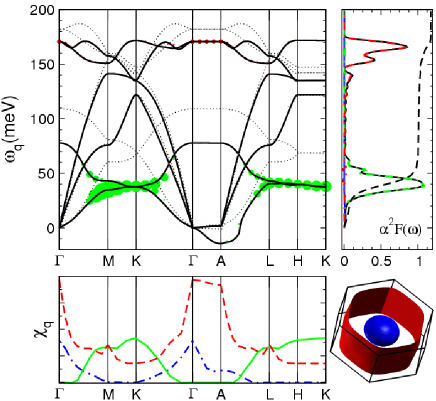
Figure 3: (Color Online) Upper left: phonon dispersions (black solid lines) for JIG with the same lattice constants $\left(c/a=\text{1.81}\right)$ and filling $n\!\!=$2/3 as in CaC₆. Thin dotted lines show the corresponding dispersions for $n\!=$0 (undoped graphite). Imaginary frequencies are shown as negative (see text). The area of a colored dot is proportional to the mode coupling constant $\lambda_{\nu\mathbf{q}}.$ Color code: red $\pi^{\ast}$ intraband; blue IL intraband (negligible); green $\mathrm{IL}\!\mathrm{-\!}\pi^{\ast}$ interband. Upper right: JIG e-ph spectral function $\alpha^{2}F(\omega)$ and $\lambda(\omega)$ defined as in Eq. 6, but integrated to $\omega$ rather than to $\infty$ (dashed). Lower left: JIG nesting functions $\chi_{nm}(\mathbf{q}).$ Lower right: Fermi surface of JIG in the first Brillouin zone (IL-sphere and $\pi^{\ast}$-cylinder).

These quantities are shown for JIG in Fig. 3; in the upper half we focus on the vibrational properties and the e-ph coupling (phonon dispersions and partial Eliashberg functions) and in the lower half on the electronic properties (nesting functions and Fermi surface).

We see that the Eliashberg function $\alpha^{2}F(\omega)$ merely has two pronunced peaks, respectively centered at $\omega\mathrm{\sim}40\,$meV and $\omega\mathrm{\sim}160\,$meV. The first involves the carbon out-of-plane, zone-boundary modes, and the second involves the in-plane bond-stretching, zone-center modes. The same two peaks (compare our Fig. 3 with Fig. 3 of Ref. CaC6:calandra:band, ) are found in the $\alpha^{2}F(\omega)$ of CaC₆, which, of course, also has an additional low-frequency peak involving in-plane vibrations of Ca.

Integrating $\alpha^{2}F(\omega)/\omega$ over positive frequencies lambdaNOTE yields: $\lambda\mathrm{=}1.1$, thus even larger than in CaC${}_{6},$ where $\lambda\mathrm{=}0.84,$ despite the absence of the calcium modes. We have thus shown that a large e-ph interaction survives in JIG even after removing the intercalants, whereas all the recent studies on superconductivity in GICs have assumed that either the mechanism for superconductivity is not conventional e-ph coupling, GIC:csanyi:band or that it is intrinsically related to the presence of the intercalant. GIC:mazin:band ; CaC6:calandra:band The discussion of possible reasons for the quantitative discrepancy between the $\lambda^{\prime}s$ of JIG and CaC₆ is postponed to the end of the section.

The Fermi surface of JIG (bottom right panel of Fig. 3) has two sheets, both of electron character: the sum of their volumes is $n\mathrm{\times}\Omega_{BZ}/2=\Omega_{BZ}/3.$ The $\pi^{\ast}$ sheet has negligible $k_{z}$-dispersion and is open, with the shape of honeycomb enclosing the vertical KM-HL BZ boundaries. Its hollow inside forms a $\Gamma$A-centered cylinder with average radius $k_{\pi^{\ast}}$ as shown in red at the lower right of Fig. 3. The IL sheet, shown in blue, is three dimensional, $\Gamma$-centered, and closed; when $n$ and $c/a$ equal those of CaC₆, as in Fig. 3, it closely approximates a sphere with radius $k_{\mathrm{IL}}$.

The e-ph interaction can take place in three channels: IL intraband, $\pi^{\ast}$ intraband, and IL-$\pi^{\ast}$ interband. The $\lambda_{\nu\mathbf{q}}$’s associated with each phonon mode (Eq. 7) are shown in the upper left of Fig. 3 by full dots with area proportional to $\lambda_{\nu\mathbf{q}}.$ The contributions from the IL and $\pi^{\ast}$ intraband scattering are respectively blue and red, consistently with the color code used for these two bands in Fig. 1 and for the corresponding Fermi surface sheets in the lower right panel of Fig. 3. The interband IL-$\pi^{\ast}$ scattering contribution, is, instead, green. The upper right of Fig. 3 shows the Eliashberg function and the lower left the nesting functions with the same decomposition scheme and color code.

Fig. 3 clearly shows that the zone-boundary out-of-plane buckling phonons with $\omega\mathrm{\sim}40\,$meV give the largest contribution to the total $\lambda$, and that the coupling is due to interband IL-$\pi^{\ast}$ coupling. The $\pi^{\ast}$ intraband coupling by the optical in-plane bond-stretching phonons C:piscanec:band cause the large $\alpha^{2}F(\omega)$ peak at $\omega\mathrm{\sim}160\,$meV. Due to the high frequency, however, this peak contributes a mere 20% to the total $\lambda$. Finally, with the absence of intercalant modes, our JIG model has no phonons with small $\left|\mathbf{q}\right|$ causing significant coupling (IL intraband and interband).

To understand the origin of the large interband e-ph matrix element in Eq. 2, we go back to the Wannier-like orbital in Fig. 2. As we saw, the IL and $\pi^{\ast}$ bands cross essentially without hybridizing (a tiny hybridization occurs only along the A-L line) because the IL Wannier-like orbital is invariant under all operations of the point group of the interstitial site, while the sign of the Wannier-like function for the $\pi^{\ast}$ band alternates within the extent of the IL function. If, however, we apply a buckling distortion to the graphene sheets, half of the $p_{z}$ orbitals are driven closer to the interstitial site where the IL orbital of Fig. 2 sits, and the other half are driven away, with the net result of a non-zero e-ph matrix element between the $\pi^{\ast}$ and IL bands (see the Appendix A, where this is demonstrated using a TB model).

In fact, we only need the e-ph matrix elements for Bloch functions at the Fermi level, and not for the entire IL band. Since the $n$=2/3 doped electrons not only go into the IL band, but also, and even more, into the $\pi^{\ast}$ band, the former is less than 1/3 full. To calculate the IL Bloch functions at $\varepsilon_{F}$ we could therefore also use the Wannier-like function for the lowest IL subband, obtained by folding the IL band into e.g. the three times smaller BZ of CaC${}_{6}.$ This function is shown in the upper part of Fig. 4 using the same contour as in Fig. 2. It is seen also to have the full point-group symmetry, and since the basis set spanning the lowest IL subband consists of the replicas of this function placed at all Ca sites, that is, at every third interstitial site, the square of this function is three times more diluted (extended) than the square of the Wannier-like function for the entire IL band. Whereas the Wannier function for the lowest IL subband has $a_{1g}$ symmetry, the ones for the two upper IL subbands have $e_{g}$ symmetry, that is, their signs alternate. So one could also say that, for these three subbands, the Wannier function can be obtained by forming the three linear combinations (of axial symmetry $a_{1g}$ and $e_{g}$) of the “small” Wannier function of the entire IL band (Fig. 2). For the lowest band this yields the “large” Wannier function shown in Fig, 4, whose axial symmetry is $a_{1g}$. The point is, that for the relatively low fillings of the IL band which are of our interest, this is the Wannier function required to form the proper Bloch IL functions at the Fermi level; and this function  is uniform on the scale of the C-C bond length. For that reason there is a large, ”dormant” IL-$\pi^{\ast}$ matrix element for buckling modes.

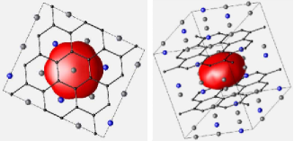
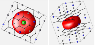
Figure 4: (Color Online) Top and side view of the Wannier-like function for the lowest of the three IL subbands, the $a_{1g}$ subband, in JIG (top) and in CaC₆ (bottom). The basis set spanning the $a_{1g}$ subband consists of the replicas of this function placed at all Ca sites, i.e., at every third interstitial site, the blue ones. The isocontour and the color scheme is the same as in Fig. 2.

III.2 JIG vs. CaC₆

How well do our results for JIG reproduce what is observed in real GICs? As an example, we consider CaC₆. Here, the IL band is folded three times into the rhombohedral BZ, and split; however, the occupied band structure of CaC₆ still bares a very close resemblance to that of JIG. GIC:csanyi:band ; GIC:mazin:band ; CaC6:calandra:band ; GICs:Mazin:review This is clearly visible in Fig. 7, where we show an in-plane cut of the Fermi surface of the two systems in the (three times smaller) rhombohedral Brillouin zone of CaC₆. CaC6structure The folding of the hexagonal BZ of primitive graphite into the rhombohedral BZ of CaC₆, shown in the left panel, may obscure the simple Fermi surface topology appearing in the lower right panel of Fig. 3, but it clarifies the origin of the complicated Fermi surface of CaC₆, shown in the right panel of Fig. 7. In both cases we clearly recognize a quasi-spherical IL Fermi surface and a more complicated structure, which, however, only amounts to folding the outer $\pi^{\ast}$ honeycombs; in the right panel only small hybridization gaps, in the $\Gamma-M$ and equivalent directions, make CaC₆ slightly different from the purely folded graphite shown at the left.

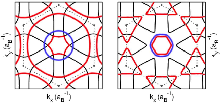
Figure 5: (Color Online) Fermi surface of JIG and of of CaC₆, both shown in the reciprocal space of rhombohedral CaC₆ (top view, compare to the 3D view of Fig. 3, lower right panel). Once folded into the three times smaller BZ, the JIG Fermi surface (left), which in the hexagonal BZ (grey dotted lines) consists of an IL sphere (blue) and a $\pi^{\ast}$ honeycomb (red), reveals remarkable similarities with that of CaC₆ (right).

This comparison suggests that the introduction of Ca atoms between the C₂ layers preserves the physical picture discussed above. This is also confirmed by the Wannier-like function for the lowest IL subband, shown in the bottom panels of Fig. 4, and is seen to be very similar to the one for the lowest subband of JIG, shown in the top panels and discussed before. The main difference is the presence of some Ca 3$d_{3z^{2}-1}$ character in the IL Wannier-like function for CaC₆, but this does not disrupt the large dormant IL-$\pi^{\ast}$ matrix element for buckling modes.

III.3 Why JIG overestimates the CaC₆ e-ph

A large e-ph interaction associated to C out-of-plane modes has been calculated in CaC₆ and several other GICs; CaC6:calandra:band ; CaC6:jskim:press ; GIC:calandra:band our JIG model gives a convincing qualitative picture of this electron-phonon interaction in CaC₆ and, as shown in the next section, also correctly explains the observed trend of $\lambda$ observed in different GICs. However, as we already pointed out, there is a large quantitative discrepancy in the values of $\lambda$, even though the electronic parameters (DOS, Fermi velocities) are comparable. As a matter of fact, in JIG we obtain an overall larger $\lambda$ than in the corresponding real GICs, even though, in JIG, the phonon modes associated to the in-plane vibrations of the intercalant, which give a sizable contribution to $\lambda$ in real intercalated graphites CaC₆, SrCa₆, and BaC₆, are missing (these calcium modes cause a strong e-ph interaction, because displacing the IL Wannier-like function off center in the $xy$-plane also awakes the dormant IL-$\pi^{\ast}$ and IL-IL couplings).

The bottomline is that, in JIG, the $\lambda$ associated to the IL-$\pi^{\ast}$ coupling via out-of-plane phonons is almost three times as large as in real GICs. Why? Most of this boost comes from the difference in phonon frequency: in real compounds, the presence of an intercalant ion partially hinders the vertical motion of C atoms, thus hardening the out-of-plane frequencies.

For example, the peak associated to C out-of-plane vibrations is at $\omega\mathrm{\sim}$55 meV in CaC₆, but at $\omega\mathrm{\sim}$40 meV in the corresponding JIG. Assuming that the partial $\lambda$ associated to this mode can be approximated by the Hopfield formula $\lambda=N(0)g^{2}/M\omega^{2}$, where $g$ is the e-ph matrix element, this would give an enhancement factor of $(55/40)^{2}$, i.e., almost two, going from real CaC₆ to JIG, if $N(0)$ and $g$ were the same in the two systems. But they are not, and the quantitative differences in the band structure which affect them (such as a weak hybridization between IL and $\pi^{\ast}$ bands, visible in CaC₆ but absent in JIG, see Fig. 7) are probably enough to explain the total enhancement factor of almost 3 found between JIG and actual CaC₆, as far as the e-ph coupling of carbon-buckling modes is concerned.

IV Effects of electron doping, $n,$ and interlayer spacing, $c.$

Csanyi et al. GIC:csanyi:band have proposed that the electronic properties of donor-intercalated GICs be mainly determined by the interlayer spacing and valence of the intercalant; recent first-principles calculations GIC:calandra:band and experiments GIC:jskim:unp suggest a possible correlation between T_c and the $c$ axis lattice constant; these hints are both confirmed and clarified in their origin by the results presented here. Having so far studied in detail the electron-phonon interaction of JIG in comparison with CaC₆, we will now turn to discuss how the two independent variables of our model, $c/a$ and $n$, affect the e-ph properties of JIG, and compare the JIG trends with the available experimental data. In the whole range of $c/a$ and $n$ considered here, there is a single interlayer band at the Fermi level (see Section I ).

Electrons: In Fig. 6 we plot the energy position of the bottom of the IL band as a function of $c/a$ for different $n$. As mentioned in Section I, the addition of a uniform, positive background of charge to graphite shifts the IL band down in energy w.r.t. the rest of the band structure, leaving its shape unaffected. The effect is obviously stronger for larger $n$. The IL band is shifted down in energy also when the $c/a$ ratio is increased. Changing the separation between the graphite planes also sensibly affects the IL bandwidth along $k_{z}$, so that the associated FS, which in CaC₆ is nearly a sphere (Fig. 3), becomes an oblate ellipsoid for smaller $c$’s. In the opposite limit (large $c$’s), the opposite happens. The same trend is observed in real GICs (see Ref. GIC:calandra:band, ).

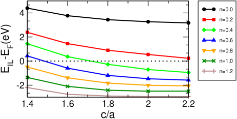
Figure 6: (Color Online) Position of bottom the IL band in JIG as a function of interlayer C spacing ($c/a$) for different electron dopings $n$; see also Fig.4 of Ref. GIC:csanyi:band, .

Phonons: In the upper left panel of Fig. 3 we show the phonon dispersions with electron doping $n$=2/3 (black solid line) and without doping ($n$=0, thin dotted line). The JIG phonon frequencies are lower than those of undoped graphite in the entire BZ, regardless of the presence or absence of e-ph coupling. Such a large, dispersionless energy shift, common to all phonons, is not due to e-ph coupling, but rather to a softening of all bonds, related to the increased filling of the $\pi^{\ast}$ antibonding states. softeningpaper Fig. 3 shows that on top of this global phonon softening, there is a further $\mathbf{q}$-dependent softening caused by e-ph interaction.

The effect of doping and the $c/a$ ratio on the frequency of the zone-center $\left(\Gamma\right)$ optical buckling modes is illustrated in the left panel of Fig. 7. For fixed $c,$ the mode softens for larger $n$, because of the filling of the antibonding $\pi^{\ast}$ band. For fixed $n$, the frequency softens at lower $c/a$, where the charge transfer to $\pi^{\ast}$ states increases, due to the emptying of the IL band (Fig. 6). In the right panel of the same figure we plot the frequency of the doubly-degenerate buckling mode at the $\left(K\right)$ point; here, on top of the softening due to charge transfer, an additional softening due to e-ph interaction takes place.

The same softening of the out-of-plane phonons with respect to pure graphite is observed also in real GICs, where the effect is partially compensated by the presence of the intercalant, which hinders the vertical motion of the C atoms. However, in some cases the effect depicted in Fig. 7 is so strong as to lead to structural instabilities also in actual compounds. An extreme example in this sense is LiC₂, for which, using the lattice parameters of Ref. GIC:lang:theory, , we found imaginary frequencies in the entire BZ for both the acoustical out-of-plane and the optical buckling branch. Fig. 7 further suggests that many compounds with chemical formula AC₂ may be dynamically unstable for this mechanism.

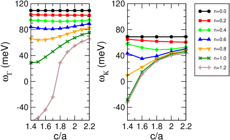
Figure 7: (Color Online) Frequency of the optical buckling mode at $\Gamma$ (left) and K (right) as a function of the $c/a$ ratio for JIG, at different dopings $n$; the in-plane lattice constant is that of CaC${}_{6},$ for which $c/a$=1.81 and $n$=2/3. Symbols represent calculated data, lines are meant to guide the eye. Imaginary frequencies are shown as negative.

Electron-phonon coupling: We have just seen that the largest source of e-ph coupling in JIG is the interband IL-$\pi^{\ast}$ channel, and that $c/a$ and $n$ critically affect the relevant electronic bands and phonon modes. To understand how this can affect the e-ph properties, we observe that, in general, $\lambda$ will benefit from three factors: the filling of the IL band (Fig. 6), the softening of the out-of-plane phonon frequencies (Fig. 7), and an increase of the IL-$\pi^{\ast}$ electron-phonon matrix element ($g$), which grows as the graphene layers are squeezed together (not shown). This suggests that a promising route to increase T_c is either to increase the electron concentration - but this route is severely limited by lattice instabilities - or to reduce the $c/a$ ratio, by applying pressure or intercalating smaller atoms. Notice however that even in the second route $\lambda$ cannot be increased beyond a threshold value, because as $c/a$ is reduced the IL band is gradually emptied (see Fig. 6). Experiments have indeed shown that pressure can increase T_c in these compounds; but this route is unfortunately limited by the appearance of instabilities in the vibrational spectrum. CaC6:gauzzi:press ; CaC6:jskim:press ; GIC:calandra:band

To gain a consistent picture of how the interplay of the three factors affects the e-ph interaction in JIG, we study the Eliashberg function and the frequency-dependent $\lambda(\omega)$ as a function of $c$, with $a$ and $n$ fixed at their values in CaC₆. In the $c$-range considered, both the position and the shape of the high-frequency peak, which involves the $\pi^{\ast}$-$\pi^{\ast}$ coupled bond-stretching modes, is nearly independent of $c$. For the low-frequency peak, involving the IL-$\pi^{\ast}$ coupled buckling modes, the situation is entirely different. For the three higher values $c/a$=1.81, 2.00, 2.11 which match those of real GICs (CaC₆, SrC₆ and BaC₆) latticeNOTE for which first-principles calculations are available,GIC:calandra:band the contribution to $\lambda$ from the low-frequency peak decreases with increasing $c$: as the graphene layers are pulled apart, the overlap between the IL and $\pi^{\ast}$ wavefunctions decreases, the e-ph matrix-element of Eq. 2 gets smaller, the buckling modes get harder. Below $c$=1.35$a$, on the other hand, the low-frequency peak is just absent, because, at $n$=2/3, the IL band is empty, and gives no contribution to $\lambda$; so at first, as $c$ increases beyond 1.35$a,$ the e-ph interaction must increase, because, with the growing size of the IL sheet, the density of states entering Eq. 4 grows. As a consequence $\lambda$, and thus $T_{c}$, will (for $n$=2/3) have a maximum for some $1.35\!<\!c/a\!<1.81$, which we calculated around 1.6 and is also shown in Fig. 8.

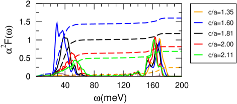
Figure 8: (Color Online) JIG Eliashberg function $\alpha^{2}F(\omega)$ (solid lines) and frequency-dependent $\lambda(\omega)$ (Eq. 6, but only up to $\omega$: dashed lines) for fixed $n\!$=2/3 and different $c$ and with $a$ fixed at its value in CaC${}_{6}.$ For $c/a\!\leq$1.35 the IL band is empty and the low-frequency peak associated with the out-of-plane C vibrations is absent. As $c/a$ grows from its value (1.81) in CaC₆ to the one in BaC₆ (2.11), this peak shifts to higher frequency and its weight dramatically drops, while the high-frequency peak of the in-plane modes, remains unchanged. Reducing $c/a$ to $1.6$, instead, causes an increase in $\lambda$.

Our calculated JIG trend for $\lambda$ matches that of the real compounds (see Fig. 7 of Ref. GIC:calandra:band, ). Details are given in Table 1, which also shows that although this trend is the right one, the total $\lambda$ in JIG is consistently larger than that of the corresponding GIC. For a discussion of the possible reasons for this discrepancy, see the end of the previous section.

	$c/a$	EIL-EF	$N(0)$	$\lambda$
JIG	1.35	-0.48	0.04	0.2
JIG	1.60	0.93	0.10	1.6
JIG	1.81	1.44	0.12	1.1
JIG	2.00	1.66	0.14	0.8
JIG	2.11	1.81	0.16	0.7
CaC6 †	1.81	1.25	0.13	0.83
SrC6 $\;{}^{{\dagger}}$	2.00	1.66	0.14	0.54
BaC6 †	2.11	1.46	0.12	0.38

Table 1: Comparison of JIG with $n\!$=2/3 (this work) with real alkali-metal intercalated graphites with $n\!$=2/3 (Ref.  GIC:calandra:band, ). $E_{IL}$ is the energy of the bottom of the IL band (eV). $N\left(0\right)$ is the total DOS in states/(eV $\!\!\cdot\!\!$ C spin). The corresponding $\alpha^{2}F(\omega)$ are in Fig. 8.
The data marked with ^† are taken from Ref.  GIC:calandra:band, ; their e-ph coupling $\lambda$ also includes intercalant-related modes, which contribute almost half the total coupling.

V Conclusion

In this paper we have studied the e-ph properties of electron-doped graphite, using a jellium model in which the excess electrons are neutralized by a uniform positive background of charge. We have shown that, despite its simplicity, the proposed model identifies and explains an important source of the e-ph interaction in real GICs, namely, the existence of an interlayer (IL) three-dimensional electronic band, whose filling determines the occurrence of a strong, otherwise dormant e-ph interaction between IL and $\pi^{\ast}$ electrons, for which we provided a simple understanding in terms of Wannier-like functions. Our picture corrects the rough idea according to which, since IL states are free-electron like, they must experience little or no interaction with the electronic states and phonon modes related to the carbon layers. We have shown that, on the contrary, IL states can experience a strong interaction with the surrounding C lattice, and thus give sizable contribution to the e-ph coupling, as observed in GICs, CaAlSi:gianto:band disilicides and metal-sandwich structures. LiB:curtarolo:band ; LiB:mazin:band Our results amount to a natural explanation for the empirical correlation between the filling of the IL band and the occurrence of superconductivity in the GICs, and nicely fit the observed correlation between T_c and layer spacing in actual GICs.

Moreover, since $\pi^{\ast}$ and IL electronic bands as well as carbon out-of-plane phonon modes are found in several other materials, from nanotubes NFES_in_CNTs to layered compounds, CaAlSi:gianto:band including the recently proposed metal sandwich structures, LiB:curtarolo:band ; LiB:mazin:band our findings may represent an inspiration for further research on the electron-phonon mechanism identified here.

VI Acknowledgements

We thank F. Mauri and S. Massidda for useful discussion, and Igor I. Mazin for suggestions and a critical reading of our manuscript. One of us (GBB) gratefully acknowledges partial financial support from MUR (the Italian Ministry for University and Research) through COFIN2005.

Appendix A: Tight-binding Model

Undistorted JIG

The NMTO method Theory:andersen:TBLMTOASA ; Theory:andersen:NMTO allows us to define from first principles three most localized “atomic” orbitals which span the Hilbert space of the electronic states corresponding to three bands which, in the main paper, were labeled as $\pi$, $\pi^{*}$, IL, and associated to the e-ph interaction in GICs. What do they look like and where do they sit? To answer this question we need the geometry of our JIG model. “Primitive graphite” C₂ has $\alpha\alpha\alpha$ stacking; direct and reciprocal lattices are defined by the basis vectors

$$\left[\begin{array}[]{c}\mathbf{T}_{1}\\ \mathbf{T}_{2}\\ \mathbf{T}_{3}\end{array}\right]=\left[\begin{array}[]{ccc}\frac{a\sqrt{3}}{2}&\frac{a}{2}&0\\ 0&a&0\\ 0&0&{c}\end{array}\right];\left[\begin{array}[]{c}\mathbf{G}_{1}\\ \mathbf{G}_{2}\\ \mathbf{G}_{3}\end{array}\right]=2\pi\left[\begin{array}[]{ccc}\frac{2}{a\sqrt{3}}&0&0\\ -\frac{1}{a\sqrt{3}}&\frac{1}{a}&0\\ 0&0&\frac{1}{c}\end{array}\right]\,;$$

the positions of the two C atoms within the unit cell are

$$\pm\mathbf{C\equiv}\pm\frac{1}{3}\left(\frac{\mathbf{T}_{1}}{2}-\frac{\mathbf{T}_{2}\!-\!\mathbf{T}_{1}}{2}\right)=\left(\frac{\pm a}{2\sqrt{3}},0,0\right)\,,$$

and the position of the interstitial site S, where the intercalant may sit in real GICs, is:

$$\mathbf{S\equiv}\frac{1}{2}\mathbf{T}_{3}=\left(0,0,\frac{c}{2}\right).$$

Out of our three localized orbitals, two sit on the two carbon atoms of the C₂ unit cell, are of $p_{z}$ symmetry, and are naturally identified with the carbon $p_{z}$ orbitals; the third sits on the interstitial site and, although it looks like an $s$ orbital (see Fig. 2), has only axial symmetry (around $z$); for simplicity of notation, however, we assign it an $s$ subscript, keeping in mind that this is not a purely $s$ orbital:

$$\left\langle\mathbf{r}|\pm\mathbf{C}\right\rangle=\psi_{p_{z}}(\mathbf{r}\mp\mathbf{C})\quad;\quad\left\langle\mathbf{r}|\mathbf{S}\right\rangle=\psi_{s}(\mathbf{r}-\mathbf{S})\,.$$

If we diagonalize the electronic hamiltonian $\hat{h}$ in the $3\!\times\!3$ basis of the localized states $|+\mathbf{C}\rangle$, $|-\mathbf{C}\rangle$, and $|\mathbf{S}\rangle$, or, more precisely, of the three corresponding Bloch sums

$$\left|{\pm{\mathbf{C,k}}}\right\rangle = \sum_{\mathbf{T}}\mathrm{e}^{i\mathbf{k\cdot T}}\left|\mathbf{T}\!\pm\!\mathbf{C}\right\rangle$$ (8)

$$\left|{\mathbf{S},\mathbf{k}}\right\rangle = \sum_{\mathbf{T}}\mathrm{e}^{i\mathbf{k\cdot T}}\left|\mathbf{{T}+{S}}\right\rangle$$ (9)

where the sum extends to all lattice vectors $\mathbf{T}$, we recover, by construction, the three electronic bands ($\pi$, $\pi^{\ast}$ and IL) from which these localized states were derived, and obtain the corresponding Bloch states ($|\pi;\mathbf{k}\rangle,|\pi^{\ast};\mathbf{k}\rangle$ and $|\mathrm{IL};\mathbf{k}\rangle$) as a linear combination of these three Bloch sums. The three relevant NMTO bands are shown as red dashed lines in the upper panels of Fig. 9 for our JIG without (left) and with (right) a $\Gamma$-point buckling phonon displacement of 0.17 a.u.; the full JIG band structure from pseudopotentials and plane waves is shown as black solid lines, for comparison. With our $3\!\times\!3$ basis, an essentialy perfect “first-principles” tight-binding representation is obtained by truncating the electronic hamiltonian matrix beyond the sixth shell of nearest neighbors (n.n.), and shown by the green dotted lines in the upper panels of Fig 9. The corresponding formulae and parameters are available upon request. askLilia

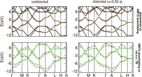
Figure 9: (Color Online) Band structures of undistorted (left) and phonon-distorted (right) JIG (see text). Here the energy zero is at the Fermi energy. Upper panels: comparison of the full band structure based on plane waves and pseudopotentials (black solid) with the three ($\pi$, $\pi^{\ast}$ and IL) minimal downfolded bands (red dashed) obtained from a (3x3) NMTO. As green dotted lines we also show the corresponding $6^{th}$-n.n. tight-binding bands. Lower panels: we reproduce the three relevant NMTO bands of the upper panels, and compare them with 1^st-n.n. first-principle tight-binding bands (green solid). These bands look obviously poorer than those with 6 neighbors, but they still correctly reproduce the band splittings due to the phonon displacement (see text).

Table 2: $3\!\times\!3$ nearest-neighbor first-principles TB parameters for undistorted JIG, from NMTO (see text and Table 3), in eV. Unlike Fig. 9, here the energy zero is at the crossing point of the $\pi$ and $\pi^{*}$ bands, so E${}_{F}=$ 2.0 eV. A carbon-buckling phonon of amplitude $u=0.02\,a$ (where $a$ is the planar lattice constant of C₂) changes $t_{sp}$ by as much as $0.1122$ eV. To linear order this means $\delta t_{sp}/\delta u=2.241$ eV/Å.

$\varepsilon_{s}-\varepsilon_{p}\phantom{-}=\phantom{-}3.5115$	$t_{sp}=\,\,0.8155$
$\theta_{s}=\theta_{s}^{xy}\,\,=-0.8811$	$t_{pp}\,\,=\,\,t_{pp}^{xy}=\,\,2.5626$

Table 3: The $3\!\times\!3$ electronic hamiltonian for JIG when only nearest neighbor integrals (see Table 2 and text) are retained.

		$\left|\mathbf{S};\mathbf{k}\right\rangle$		$\left|\mathbf{C};\mathbf{k}\right\rangle$		$\left|-\mathbf{C};\mathbf{k}\right\rangle$
$\left\langle\mathbf{S};\mathbf{k}\right|$		$(\varepsilon_{s}\!-\!\varepsilon_{p})+2\theta_{s}\left[\cos(2\lambda)+\cos(2\mu)+\cos(2\nu)\right]$		$-2ie^{-i\xi}t_{sp}\sin(\xi)\left(1+e^{-2i\mu}\!\!+e^{-2i\nu}\right)$		$-2ie^{-i\xi}t_{sp}\sin(\xi)\left(1+e^{-2i\mu}\!\!+e^{-2i\lambda}\right)$
$\left\langle\mathbf{C};\mathbf{k}\right|$		$2ie^{i\xi}t_{sp}\sin(\xi)\left(1+e^{2i\mu}+e^{2i\nu}\right)$		0		$-t_{pp}(1+e^{2i\lambda}+e^{-2i\nu})$
$\left\langle\mathbf{-C};\mathbf{k}\right|$		$2ie^{i\xi}t_{sp}\sin(\xi)\left(1+e^{2i\mu}+e^{2i\lambda}\right)$		$-t_{pp}(1+e^{-2i\lambda}+e^{2i\nu})$		0

However, to understand the basic features of the band structure and e-ph interaction, nearest-neighbor matrix elements may be enough. In this case only a few integrals survive: if $\alpha$ and $\beta$ equal $s$ for the $|\mathbf{S}\rangle$ orbital which sit on the interstitial site and $p$ for the two carbon $|\pm\mathbf{C}\rangle$ orbitals, we have onsite hopping integrals indicated by $\varepsilon_{\alpha}$ and $\varepsilon_{\beta}$, hopping integrals between orbitals of types $\alpha,\beta$ sitting on n.n. atoms indicated by $t_{\alpha\beta}$ (and all taken positive, $t\equiv\left|t\right|$), and hopping integrals between orbitals of type $\alpha$ sitting on the same atom of n.n. unit cells indicated by $\theta_{\alpha}$. Their numerical values are in Table 2.

Then the hamiltonian matrix is given by Table 3, where

$$\lambda\equiv\mathbf{k}\cdot{\displaystyle\frac{\mathbf{T}_{1}}{2}}={\displaystyle\frac{a}{4}}\left(k_{y}\!+\!\sqrt{3}k_{x}\right),\quad\mu\equiv\mathbf{k}\cdot{\displaystyle\frac{\mathbf{T}_{2}}{2}}={\displaystyle\frac{a}{2}}\,k_{y}\,,$$

$$\nu\equiv\mathbf{k}\cdot{\displaystyle\frac{\mathbf{T}_{2}\!-\!\mathbf{T}_{1}}{2}}=\mu-\lambda={\displaystyle\frac{a}{4}}\left(k_{y}\!-\!\sqrt{3}k_{x}\right),$$

$$\xi\equiv\mathbf{k}\cdot{\displaystyle\frac{\mathbf{T}_{3}}{2}}={\displaystyle\frac{c}{2}}\,k_{z}\,;$$

the corresponding n.n. bands are shown as solid green lines in the lower panels of Fig. 9, where they are compared to the original NMTO bands (red dashed). Notice that, in this model, the $k_{z}$ dispersion entirely comes from the $s\!-\!p$ hopping between the $s$ orbital sitting on the interstitial site and the carbon $p_{z}$ orbitals on the graphite planes immediately above and below it: carbon $p\!-\!p$ matrix elements between adjacent graphite planes are beyond n.n. In the $k_{z}\!\!=\!\!0$ plane ($\xi\!\!=\!\!0$) the matrix element between $s$ and $p_{z}$ orbitals is identically zero, because the phases of the $p_{z}$ orbitals on two adjacent graphene sheets cancel. Therefore, for $k_{z}\!\!=\!\!0$, the IL band is

$$\varepsilon_{\mathrm{IL}}(\mathbf{k})=\varepsilon_{s}+2\theta_{s}\biggl{[}\cos\left(\frac{k_{y}a+\sqrt{3}k_{x}a}{2}\right)+\cos k_{y}a$$

$$+\cos\left(\frac{k_{y}a-\sqrt{3}k_{x}a}{2}\right)\biggr{]}\,,$$ (10)

and its eigenvector $|\mathrm{IL};\mathbf{k}\rangle=|\mathbf{S};\mathbf{k}\rangle$ just coincides with the Bloch sum of Eq. 9; the $\pi,\pi^{*}$ bands entirely derive from the $p_{z}$ sub-block, whose diagonalization yields:

$$\varepsilon_{\pi^{*},\pi}(\mathbf{k})=\varepsilon_{\pi\mp}(\mathbf{k})=\varepsilon_{p}\pm t_{pp}\left|1+e^{2i\lambda}+e^{-2i\nu}\right|=$$ (11)

$$=\varepsilon_{p}\pm t_{pp}\sqrt{3+4\cos\frac{k_{y}a}{2}\cos\frac{\sqrt{3}k_{x}a}{2}+2\cos k_{y}a}$$

with eigenvectors

$$\left|\pi^{*};\mathbf{k}\right\rangle = \left|\pi_{-};\mathbf{k}\right\rangle=\frac{1}{\sqrt{2}}\left\{\left|-\mathbf{C};\mathbf{k}\right\rangle e^{i\varphi\left(\mathbf{k}\right)}-\left|\mathbf{C};\mathbf{k}\right\rangle e^{-i\varphi\left(\mathbf{k}\right)}\right\}$$

$$\left|\pi\phantom{{}^{*}};\mathbf{k}\right\rangle = \left|\pi_{+};\mathbf{k}\right\rangle=\frac{1}{\sqrt{2}}\left\{\left|-\mathbf{C};\mathbf{k}\right\rangle e^{i\varphi\left(\mathbf{k}\right)}+\left|\mathbf{C};\mathbf{k}\right\rangle e^{-i\varphi\left(\mathbf{k}\right)}\right\},\quad$$

where $2\varphi\left(\mathbf{k}\right)$ is the phase of $\left(1+e^{2i\lambda}+e^{-2i\nu}\right)$. The state $\left|\pi_{+}\right\rangle$ has lower eigenvalue and is of bonding character, being a bonding combination of the carbon ${p_{z}}$ orbitals at $\mathbf{k}=0$; the other one, $\left|\pi_{-}\right\rangle$, is the antibonding combination. In Fig. 10 we show a real-space cartoon of these three complex Bloch sums, only in the $xy$ plane; in the vertical direction (not shown) both Bloch sums $|\pi_{\pm};\mathbf{k}\rangle$ are odd with respect to the plane, since both derive from $p_{z}$ states; orbitals on different planes differ by a phase factor $e^{2i\xi}$.

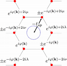
Figure 10: (Color Online) Schematic real-space picture of the three Bloch sums $|\mathbf{S};\mathbf{k}\rangle$ and $|\pi_{\pm};\mathbf{k}\rangle$ in a single graphitic plane (see text). Red dots mark the position of carbon atoms; the blue dotted circle represents the interstitial localized orbital $|\mathbf{S}\rangle$ sitting in the central unit cell; similar wavefunctions are at the center of all other unit cells, multiplied by an appropriate phase factor, but are not shown here. In the vertical (out-of-plane) direction, wavefunctions are multiplied by an additional phase factor $e^{2i\xi}$.

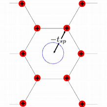
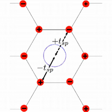
Figure 11: (Color Online) Schematic real-space picture, in the $xy$ plane, of the Bloch sums $|\mathbf{S};\mathbf{k}\rangle$, $|\pi_{+};\mathbf{k}\rangle$ (left), and $|\pi_{-};\mathbf{k}\rangle$ (right), for $k_{x}\!=\!k_{y}\!=\!0\rightarrow\varphi(\mathbf{k})=0$ ($\Gamma-A$ line).

For $k_{z}\!\!\neq 0\!\!$   the matrix element between $s$ and $p_{z}$ states is not zero, so, unlike the $k_{z}\!\!=0\!\!$   case, the $|\mathbf{S};\mathbf{k}\rangle$ and $|\pi_{\pm};\mathbf{k}\rangle$ Bloch sums may hybridize. A priori this means that the matrix elements of the electronic hamiltonian $\langle\pi_{\pm};\mathbf{k}|\hat{h}|\mathbf{S};\mathbf{k}\rangle$ may be nonzero; however it turns out that one of the two, the antibonding Bloch sum, gives $\langle\pi_{-};\mathbf{k}|\hat{h}|\mathbf{S};\mathbf{k}\rangle=0$ almost everywhere. The only exception is a tiny $\mathbf{k}$-space region between the $A$ and $L$ points; the corresponding, small gap between the $\pi^{*}$ and the IL bands is visible in Fig. 9 but not in Fig. 1, because of the thickness of the “fat bands”. The reason why $\langle\pi_{-};\mathbf{k}|\hat{h}|\mathbf{S};\mathbf{k}\rangle=0$ may be immediately understood along the $\Gamma\!-\!A$ line ($k_{x}\!=\!k_{y}\!=\!0$), where $\varphi(\mathbf{k})\!=\!0$ (see Fig. 11, where we display the three corresponding Bloch sums): each $\mathbf{S}$ site has 12 carbon nearest neighbors, 6 above and 6 below, which respectively carry, in the vertical direction, phase factors of 1 and $e^{2i\xi}$, so for the bonding ($+$) and antibonding ($-$) Bloch sums we obtain:

$$\langle\pi_{+};\mathbf{k}|\hat{h}|\mathbf{S};\mathbf{k}\rangle = -\frac{1}{\sqrt{2}}\left(6t_{sp}+6t_{sp}e^{2i\xi}\right)$$

$$\langle\pi_{-};\mathbf{k}|\hat{h}|\mathbf{S};\mathbf{k}\rangle = -\frac{1}{\sqrt{2}}\!\left[3t_{sp}-3t_{sp}+(3t_{sp}-3t_{sp})e^{2i\xi}\right]=0$$

However, even for any other $\mathbf{k}$ point in the Brillouin zone (BZ) a similar, just more lengthy procedure, based on the phases of Fig. 10, gives zero for the antibonding Bloch sum; except, as mentioned, in a small region between the $A$ and $L$ points, where the definition of bonding and antibonding looses its meaning. In other words, the electronic states corresponding to the $\pi^{*}$ band may legitimately be identified with the $|\pi_{-};\mathbf{k}\rangle$ Bloch sum of $p_{z}$ orbitals over almost the entire BZ, with no or very little admixture of the Bloch sum of the interstitial orbitals $|\mathbf{S};\mathbf{k}\rangle$.

Distorted JIG

We have seen that, in the undistorted lattice, the matrix element of the electronic hamiltonian between the Bloch sum of interstitial orbitals $|\mathbf{S};\mathbf{k}\rangle$ and the antibonding Bloch sum $|\pi_{-};\mathbf{k}\rangle$ is almost always zero, so that the latter can be practically identified as the Bloch state of the $\pi^{*}$, while the Bloch state of the IL band will have a prevailing $|\mathbf{S};\mathbf{k}\rangle$ character plus, at certain $\mathbf{k}$’s, some admixture of the bonding $|\pi_{+};\mathbf{k}\rangle$ Bloch sum. Upon out-of-plane distortions of the graphene sheets, our e-ph ab-initio calculations reveal, instead (see main paper), a large coupling between the the $\pi^{*}$ band and the IL band. How do we understand that? By symmetry: in graphene the relevant out-of-plane phonons have the same symmetry as the $\pi^{*}$ electronic states. The relevance of this symmetry argument appears if we estimate the e-ph coupling between the electronic states $i$ and $j$ due to the phonon mode ($\nu\mathbf{q}$) with the change of the corresponding electronic matrix element upon phonon displacement

$$\left\langle i,\mathbf{k}\right|\delta\hat{h}_{\nu\mathbf{q}}\left|j,\mathbf{k+q}\right\rangle,$$

multiplied by the nesting function $\delta(\varepsilon_{i\mathbf{k}})\delta(\varepsilon_{j\mathbf{k+q}})$ and integrated over the Fermi surface. Within our nearest-neighbor model this well defined, but not immediate procedure, ultimately recovers the high coupling obtained in the full first-principles calculation (see main paper). But at special points in the BZ our model allows to understand the underlying symmetry argument by inspection. The simplest example is the $\Gamma$ optical buckling phonon ($\mathbf{q}\!=\!0$). This is the frozen-in distortion considered in the right panels of Fig. 9, whose most visible effect on the electronic states is the appearance of a hybridization gap between the $\pi^{*}$ and IL bands at $\sim 2$ eV above the Fermi energy, in the middle of the $\Gamma\!-\!K$ and $\Gamma\!-\!M$ lines. If, upon a $\mathbf{q}\!=\!0$ phonon distortion, the electronic hamiltonian is written as $\hat{h}_{u}=\hat{h}_{u=0}+\delta\hat{h}_{u}$, then for a general $\mathbf{k}\!\neq\!0$ the change in the electronic matrix element relevant to the e-ph coupling becomes $\left\langle i,\mathbf{k}\right|\delta\hat{h}_{u}\left|j,\mathbf{k}\right\rangle$ and is given in Table 4. From it one may already get some intuition of the strong coupling between the $\pi^{*}$ band and the IL band.

		$\left|\mathbf{S};\mathbf{k}\right\rangle$		$\left|\mathbf{C};\mathbf{k}\right\rangle$		$\left|-\mathbf{C};\mathbf{k}\right\rangle$
$\left\langle\mathbf{S};\mathbf{k}\right|$		0		$2e^{-i\xi}\delta t_{sp}\cos(\xi)\left(1+e^{-2i\mu}+e^{-2i\nu}\right)$		$-2e^{-i\xi}\delta t_{sp}\cos(\xi)\left(1+e^{-2i\mu}+e^{-2i\lambda}\right)$
$\left\langle\mathbf{C};\mathbf{k}\right|$		$2e^{i\xi}\delta t_{sp}\cos(\xi)\left(1+1+e^{2i\mu}+e^{2i\nu}\right)$		0		0
$\left\langle\mathbf{-C};\mathbf{k}\right|$		$-2e^{i\xi}\delta t_{sp}\cos(\xi)\left(1+e^{2i\mu}+e^{2i\lambda}\right)$		0		0

Table 4: Change in the JIG nearest-neighbor tight-binding electronic hamiltonian matrix elements under a $\Gamma$-buckling-phonon distortion (see text and Tables 2 and 3).

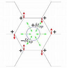
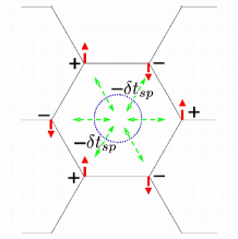
Figure 12: (Color Online) Schematic picture, in the $xy$ plane, of the Bloch sums $|\mathbf{S};\mathbf{k}\rangle$, $|\pi_{+};\mathbf{k}\rangle$ (left), and $|\pi_{-};\mathbf{k}\rangle$ (right), at the $\Gamma$ point of graphene with an optical buckling distortion of $\mathbf{q}\!=\!0$.

At $\mathbf{k}=0$ the symmetry argument becomes obvious: the $\delta\hat{h}_{\nu\mathbf{q}}$ induced by the optical buckling phonon (alternate raising and lowering of carbon atoms) has the same symmetry as the $|\pi^{*};\mathbf{k}\!=\!0\rangle=|\pi_{-};\mathbf{k}\!=\!0\rangle$ electronic state (alternate sign on carbon atoms, antibonding combination of $p_{z}$ orbitals); the product of two anti-bonding functions is bonding; as a result, we have a strong overlap with the IL electronic state, which, at $\mathbf{k}\!=\!0$, is the simple sum of interstitial $|\mathbf{S}\rangle$ orbitals. This is schematically shown in Fig 12. The only difference with respect to the purely electronic analysis of the previous cartoons (Figs. 10, 11) is that, besides the electronic phases, we must now consider the phonon phases too. Here $\delta t_{sp}$ indicates the change of the corresponding matrix element upon distortion; quantitatively, for a distortion amplitude $u=0.17$ a.u., the $t_{sp}$ matrix element changes by $\delta t_{sp}=0.101$ eV. For those carbon atoms which move towards the interstitial site, where $|\mathbf{S}\rangle$ sits, the matrix element becomes more negative: $-t_{sp}\to-(t_{sp}+\delta t_{sp})$; for those which move away from it, it becomes less negative: $-t_{sp}\to-(t_{sp}-\delta t_{sp})$. We then have, respectively for the bonding and antibonding Bloch sums:

$$\langle\pi_{+};\mathbf{k}\!=\!0|\delta\hat{h}_{u}|\mathbf{S};\mathbf{k}\!=\!0\rangle=$$

$$-\frac{2\delta t_{sp}}{\sqrt{2}}\left[1+(-1)+1+(-1)+1+(-1)\right]=0\,;$$

$$\langle\pi_{-};\mathbf{k}\!=\!0|\delta\hat{h}_{u}|\mathbf{S};\mathbf{k}\!=\!0\rangle=$$

$$-\frac{2\delta t_{sp}}{\sqrt{2}}\left[1-(-1)+1-(-1)+1-(-1)\right]=-\frac{12}{\sqrt{2}}\delta t_{sp}\,.$$

In conclusion, with our simple TB we obtain, at first glance for the $\Gamma$ point, and with some additional work at any point in the BZ, a simple physical picture not only for the electronic states, as seen in Figs. 10 and 11, but also for the e-ph interaction.

Appendix B: Computational Details

The results presented here were obtained within density functional theory DFT using two different ab-initio methods: for “fat bands”, Wannier-like orbitals, and tight-binding parameters, we used TB-LMTO-ASA Theory:andersen:TBLMTOASA and NMTO, Theory:andersen:NMTO and for total energies, phonon frequencies and e-ph couplings, we employed plane-waves and pseudopotentials. PWscf All methods give the same results for the electronic bands, the Fermi surface, and several other properties, as was carefully cross-checked.

For the self-consistent calculation of the band structure, Fermi surfaces, phonon dispersions and e-ph coupling PWscf of jellium-doped graphite we employed ultra-soft carbon pseudopotentials, Vanderbilt with a cutoff or 30 (360) Ryd for the wave-functions (density) respectively, and PBE exchange-correlation functional. DFT:PBE For the $\mathbf{k}$-space integration of the self-consistent calculations we employed a $16\times 16\times 8$ Monkhorst-Pack grid, MPgrid yielding 150 points in the IBZ, with a 0.06 Ryd cold smearing; Marzari:coldsmearing a much denser $32\times 32\times 16$ grid was used for the integration on the Fermi surface of the e-ph matrix elements. This led to a convergence of $\mathrm{\sim}1$ meV for the phonon frequencies, except for the acoustical out-of-plane branch along the $\Gamma\!-\!A$ line, which requires a much higher cutoff to converge. For consistency check, we also calculated the $\Gamma-$point frequencies of graphite in the experimental structure, obtaining frequencies within $\pm 0.1\,$meV of Ref graf:marzari:band, . Dynamical matrices and phonon linewidths were calculated on a $16\times 16\times 8$ grid in $\mathbf{q}$-space and the phonon dispersions were then obtained by Fourier interpolation. Such a dense mesh in $\mathbf{q}$-space was necessary to resolve the effect of the Fermi surface nesting on the e-ph coupling (Fig. 3).

For the fat bands and Wannier-like orbitals, we used the TB-LMTO and NMTO methods. Theory:andersen:TBLMTOASA ; Theory:andersen:NMTO In this case, to obtain a good representation of the electronic wavefunction both in the neighborhood of C atoms and in the interstitial regions, we had, in our C₂ unit cell, an $s,p,d$ basis set on each C atom, but also two “empty spheres” (with $s,p$ channels): one, small, in the C plane; another, very large, between the planes, on the interstitial site called $\mathbf{S}$ in appendix A, whose crystal coordinates are $(0,0,\frac{c}{2})$. This is where the intercalant may sit in real GICs: for example, on each of these interstitial sites in LiC₂; on every third such sites in CaC₆.

References

- (1) T. E. Weller, M. Ellerby, S. S. Saxena, R. P. Smith, and N. T. Skipper, Nature Physics 1, 39 (2005).
- (2) N. Emery et al., Phys. Rev. Lett. 95, 087003 (2005).
- (3) J. Nagamatsu, N. Nakagawa, T. Muranaka, Y. Zenitani and J. Akimitsu, Nature (London) 410, 63 (2001).
- (4) J. M. An, W. E. Pickett, Phys. Rev. Lett. 86, 4366 (2001).
- (5) J. Kortus et al., Phys. Rev. Lett. 86, 4656 (2001).
- (6) Y. Kong, O. V. Dolgov, O. Jepsen, and O. K. Andersen, Phys. Rev. B64, 020501 (R) (2001).
- (7) L. Boeri, J. Kortus, and O. K. Andersen, Phys. Rev. Lett. 93, 237002 (2004).
- (8) G. Csanyi, P. B. Littlewood, A. H. Nevidomskyy, C. J. Pickard and B. D. Simons, Nature Phys. 1, 42 (2005).
- (9) M. Posternak, A. Baldereschi, A. J. Freeman, E. Wimmer, and M. Weinert, Phys. Rev. Lett. 50, 761 (1983).
- (10) Th. Fauster, F. J. Himpsel, J. E. Fischer, and E. W. Plummer, Phys. Rev. Lett. 51, 430 (1983).
- (11) J. S. Kim, R. K. Kremer, L. Boeri, and F. S. Razavi, Phys. Rev. Lett. 96, 217002 (2006).
- (12) G. Lamura, M. Aurino, G. Cifariello, E. Di Gennaro, A. Andreone, N. Emery, C. Hrold, J.-F. March, and P. Lagrange, Phys. Rev. Lett. 96, 107008 (2006).
- (13) I. I. Mazin, Phys. Rev. Lett. 95, 227001 (2005).
- (14) M. Calandra and F. Mauri, Phys. Rev. Lett. 95, 237002 (2005).
- (15) J. S. Kim, L. Boeri, R. K. Kremer and F. S. Razavi, Phys. Rev. B 74, 214513 (2006).
- (16) L. Zhang, Y. Xie, T. Cui, Y. Li, Z He, Y. Ma and G. Zou, Phys. Rev. B 74, 184519 (2006).
- (17) I. I. Mazin, L. Boeri, O. V. Dolgov, A. A. Golubov, G. B. Bachelet, M. Giantomassi, and O. K. Andersen, condmat/0606404.
- (18) W. Kohn and L. J. Sham, Phys. Rev. 40, A 1133, (1965); P. Hohenberg and W. Kohn, Phys. Rev. B 136, 864, (1964).
- (19) N. I. Medvedeva, A. L. Ivanovskii, J. E. Medvedeva and A. J. Freeman, Phys. Rev. B 64, 020502 (2001).
- (20) M. Giantomassi, L. Boeri, and G. B. Bachelet, Phys. Rev. B 72, 224512 (2005).
- (21) A. Kolmogorov and S. Curtarolo, Phys. Rev. B 73, R180501 (2006).
- (22) Amy Y. Liu, I. I. Mazin, cond-mat/0610057.
- (23) E. R. Margine and V. H. Crespi, Phys. Rev. Lett. 96, 196803 (2006).
- (24) S. Baroni, S. de Gironcoli, A. Dal Corso, and P. Giannozzi, Rev. Mod. Phys. 73, 515, (2001). URL http://www.pwscf.org.
- (25) O. K. Andersen and O. Jepsen, Phys. Rev. Lett. 53, 2571 (1984).
- (26) O. K. Andersen, T. Saha-Dasgupta, Phys. Rev. B62, R16219 (2000) and references therein.
- (27) The width, of a fat band is proportional to the character, or of the spherical-harmonics expansion around site of the Bloch state, with the partial wave normalized to unity in the chosen atomic sphere O. Jepsen and O.K. Andersen, Z. f. Physik B 97, 35-47 (1995).
- (28) In CaC6, the Ca atoms sit between the carbon layers, occupying in turn one of the three equivalent positions at the center of the hexagons, which we shall call interstitial sites in the following; the stacking is thus (), and the smallest corresponding unit cell is rhombohedral (space group 166), with rhombohedral angle 49.55o and lattice parameter 5.17 . If we neglect the Ca ions, the resulting carbon sublattice (C6) yields a primitive graphite structure (space group 191), with and (C2).
- (29) C. Kittel, Introduction to Solid State Physics (John Wiley & Sons, New York, 1966).
- (30) With the NMTO downfolding method we obtain a minimal basis set which spans the three , and IL bands as shown red in the upper part of Fig. 8. This basis consists of two C and one E th-order muffin-tin orbital (NMTOs) per primitive cell. What is shown in Fig. 10 is the latter orbital. It is localized, -like, and centered on an interstital site (E). After symmetrical orthonormalization to all other basis funtions in the minimal set, it becomes the orbital named in Appendix A.
- (31) E. Zurek, O. Jepsen, and O.K. Andersen, ChemPhysChem 6, 1934 (2005).
- (32) For concise definitions, see Appendix A.
- (33) N. Mounet and N. Marzari, Phys. Rev. B 71, 205214 (2005).
- (34) M. Calandra and F. Mauri, Phys. Rev. B 74, 094507 (2006).
- (35) In our total , we exclude the (negligible) contributions arising from the imaginary frequencies along .
- (36) S. Piscanec, M. Lazzeri, F. Mauri, A. C. Ferrari, and J. Robertson, Phys. Rev. Lett. 93, 185503 (2004).
- (37) L. Pietronero and S. Strässler, Phys. Rev. Lett. 47, 593 (1981), C. T. Chan, W. A. Kamitakahara, K. M. Ho and P. C. Eklund, Phys. Rev. Lett. 58, 1528 (1987), C. T. Chan, K. M. Ho, and W. A. Kamitakahara Phys. Rev. B 36 3499 (1987).
- (38) L. Lang, S. Doyen-Lang, A. Charlier, and M. F. Charlier, Phys. Rev. B 49, 5672-5681 (1994) and references therein.
- (39) A. Gauzzi, S. Takashima, N. Takeshita, C. Terakura, H. Takagi, N. Emery, C. Hrold, P. Lagrange, and G. Loupias, cond-mat/0603443.
- (40) J. S. Kim et al., unpublished.
- (41) In real CaC6, SrC6 and BaC changes by less than 1 while changes by 20%. This tiny change in changes the energy of the buckling phonons by less than 0.1 meV, which is negligible, and hardens the in-plane phonons by meV.
- (42) Please send your request to the first author of this paper (L.Boeri@fkf.mpg.de).
- (43) D. Vanderbilt, Phys. Rev. B 41, R7892 (1990).
- (44) J. P. Perdew, K. Burke, and M. Ernzerhof, Phys. Rev. Lett. 78, 1396 (1997).
- (45) H.J. Monkhorst and J. D. Pack, Phys. Rev. B 13, 5188 (1976).
- (46) N. Marzari, D. Vanderbilt, A. De Vita, and M. C. Payne, Phys. Rev. Lett. 82, 3296 (1999).