Unified static renormalization-group treatment of finite-temperature crossovers close to a quantum critical point

Abstract

A nonconventional renormalization-group (RG) treatment close to and below four dimensions is used to explore, in a unified and systematic way, the low-temperature properties of a wide class of systems in the influence domain of their quantum critical point. The approach consists in a preliminary averaging over quantum degrees of freedom and a successive employment of the Wilsonian RG transformation to treat the resulting effective classical Ginzburg-Landau free energy functional. This allows us to perform a detailed study of criticality of the quantum systems under study. The emergent physics agrees, in many aspects, with the known quantum critical scenario. However a richer structure of the phase diagram appears with additional crossovers which are not captured by the traditional RG studies. In addition, in spite of the intrinsically static nature of our theory, predictions about the dynamical critical exponent, which parametrizes the link between statics and dynamics close to a continuous phase transition, are consistently derived from our static results.

I Introduction

Continuous quantum phase transitions (QPTs) constitute a very topical subject in condensed matter physics sachdev ; qpts ; sondhi ; DCqpt ; vojta-rev ; GSI and in the last few years their intensive study has stimulated interesting speculations in other branches of modern physics, too modernphys . The fundamental feature is that anomalous behaviors appear when a quantum critical point (QCP) is approached. In particular, it is now well established that the presence of such zero-temperature critical points is the key to explain unsolved puzzles in the low-temperature properties of many materials heavyfermion ; rutenati ; HTSC .

In spite of the large variety of systems that exhibit QPTs, their critical properties can be described, following the seminal paper by Hertz hertz for itinerant magnets, using suitable quantum Ginzburg-Landau (QGL) free energy functionals, characterized by the dependence of the $n$-vector order parameter field on the Matsubara-time variable $\tau$ and by the presence in the free propagator of a term related to the intrinsic dynamic of the original microscopic systems. This assures the correct inclusion of the quantum degrees of freedom, by avoiding the difficulties connected with noncommuting operators.

In the earliest works on the argument hertz ; young75 ; gerberbeck ; lawrie ; busDC80 ; gold79 ; noi-largeN ; micnas the effects of the zero-point critical fluctuations were essentially studied only at temperature $T=0$ by applying the ideas of Wilson’s renormalization-group (RG) approach.

The $T=0$ analysis does not produce additional conceptual difficulties with respect to thermal phase transitions since quantum criticality is determined by the divergence of the length scale, set by the correlation length $\xi$, as well as by the divergence of the time scale $\tau_{\xi}\sim\xi^{z}$, where $z$ is the dynamical critical exponent. The main conclusion is that, in general, a QPT in $d$ dimensions is related to a classical transition in $(d+z)$, except for Bose-like systems with ($-i\omega_{l}$) intrinsic dynamics (here $\omega_{l}$ denotes the usual bosonic Matsubara frequency: see next section). Relevant examples are the dilute Bose gas, the XY model in a transverse field and other models in the same quantum universality class sachdev ; DCqpt ; noi-largeN ; noi97 . For these peculiar systems, an unusual ($T=0$) mean-field-like quantum criticality was found for $d<2$ by variation of an appropriate control parameter (chemical potential, transverse magnetic field, and so on). This finding cannot be explained in terms of a simple dimensional crossover $d\to d+2$ but rather by means of a more complex crossover process $(d,n)\to(d=d+2,n=-2)$ involving also an effective change of the dimensionality $n$ of the order parameter field: the quantum critical exponents of the Bose-like systems can be formally obtained from those for a classical $n$-vector model with dimensionality $d+2$ and symmetry index $n=-2$ nota1 . This was conjectured in Ref. busDC80 on the grounds of a ($T=0$) RG treatment up to second order in the natural expansion parameter $\varepsilon=2-d$, proved to be valid to arbitrary order in $\varepsilon$ for the interacting Bose gas uzu and for the XY model in a transverse field kopec-chubu and confirmed by exact large-$n$-limit calculations noi-largeN ; DC82 .

It is also worth pointing out that for some systems of itinerant electrons, the Hertz theory hertz does not seem properly adequate to describe the correct $T=0$ critical behavior as will be specified in the next section. Anyway, in this paper we consider only systems for which the QGL free energy functionals are expected to describe correctly the quantum critical behavior.

The reliable and complete description of finite-temperature crossovers close to a QCP has a long history hertz ; baba ; schmeltz ; walasek ; crossovers ; millis93 ; sachdevETAL ; noi97 ; noi03 ; noi05 ; 70s ; DC82 ; walasek86 ; tvojta ; sachdev97 . Wilsonian and field-theoretic RG treatments baba ; schmeltz ; walasek ; crossovers ; millis93 ; sachdevETAL ; noi97 ; noi03 ; noi05 have been extensively used in combination with nonperturbative and self-consistent methods sachdev ; 70s ; DC82 ; walasek86 ; tvojta ; sachdev97 .

The common opinion for a long period was that, at any finite temperature, classical fluctuations control the behavior of the system, but it has become increasingly clear that the presence of a QCP peculiarly influences measurable quantities over a wide range of the low-temperature phase diagram. Indeed intricate crossovers between finite temperature regimes may occur, especially when there is a line of finite temperature phase transitions ending in a QCP. Although previous partial RG investigations of low-temperature properties and crossovers exist baba ; crossovers , the first detailed study of the low-temperature phase diagram around a QPT was performed by Millis millis93 within a RG framework treating the thermal and quantum fluctuations on the same footing. He considered quantum actions for itinerant antiferromagnets and ferromagnets and depicted the corresponding low-temperature phase diagram by solving the RG equations, step by step, in different regions selected by suitable conditions. The resulting description is correct, but the derivation of the incoming crossover lines appears cumbersome and, sometimes, rather unnatural.

In this paper we propose a nonconventional, but intrinsically simple, approach to obtain a general and systematic description of the complex structure of the phase diagram when a QCP is present, avoiding the step-by-step Millis procedure. Starting with a general QGL functional, (i) we integrate out the degrees of freedom with nonzero Matsubara frequencies, thus reducing the original quantum action to an effective classical one with temperature-dependent coupling parameters, and then (ii) we solve the related RG equations to obtain the phase diagram and the crossover scenario. It is worth mentioning that the first step has been already used by Sachdev sachdev ; sachdev97 to formulate a theoretical approach to finite-temperature quantum criticality, which mixes perturbative predictions and known $(T=0)$ RG results close to and above the quantum upper critical dimension. In our picture, the temperature-dependent effective couplings play a crucial role and we show that, with this basic ingredient, both the classical and quantum criticalities appear as a natural result of the fusion of the classical world with the underlying quantum one. This special feature, together with the powerful Wilson RG method, allows us to draw out in a unified way a series of low-temperature crossover lines, which separate different asymptotic regimes, including some which do not emerge in former approaches and which could be observable in appropriate ultralow-temperature experiments.

Moreover, within our method, we avoid the direct control of the quantum degrees of freedom in the various levels of approximation, obtaining, at the end, the quantum criticality as an emergent phenomenon. Just for this reason, we believe that the idea developed in this paper may be conveniently employed in other branches of theoretical physics, from quantum gravity to cosmology.

The paper is structured as follows. In Sec. II we introduce the quantum action which allows us to properly describe the low-temperature critical properties of many systems exhibiting a QCP. Then, after averaging over degrees of freedom with nonzero Matsubara frequencies, we present the explicit expression of the arising effective classical functional to one-loop approximation. As a second step of our program, in Sec. III the one-loop RG equations for the temperature-dependent effective coupling parameters are solved exactly close to and below four dimensions, and the general expression of the correlation function as a function of the temperature and of the original “microscopic” parameters is obtained for the quantum systems under study. Section IV is devoted to determine the critical-line equation in the low-temperature regime and the related shift exponent. The critical properties and the crossovers approaching the critical line close to the $(T=0)$ ending point (here identified as a QCP) are studied in Sec. V and their unified description in terms of two-parameters effective exponents is presented in Sec.  VI. In the next Sec. VII we localize other crossover lines far from the phase boundary to have a global picture of the phase diagram for different quantum systems. Finally, in Sec. VIII, some conclusions are drawn.

II Quantum models and effective classical Hamiltonian

A remarkable feature is that the critical properties of a wide variety of systems that exhibit QPTs can be described through a reduced number of QGL actions; each of them is representative of a given quantum universality class, defined by the space dimensionality $d$, the order parameter symmetry index $n$, and the dynamical critical exponent $z$ that characterizes the intrinsic dynamics of the systems in the class.

Bearing this in mind, in order to be as general as possible, we consider a quantum action which, in the Fourier space, is written in the form

$$S\{\vec{\psi}\} = S_{0}\{\vec{\psi}\}+S_{I}\{\vec{\psi}\}$$ (1)

$$S_{0}\{\vec{\psi}\} = \frac{1}{2}\sum_{j=1}^{n}\sum_{\vec{k},\omega_{l}}(r_{0}+k^{2}+\varphi(\vec{k},\omega_{l}))|\psi^{j}(\vec{k},\omega_{l})|^{2}$$ (2)

$$S_{I}\{\vec{\psi}\} = \frac{u_{0}T}{4V}\sum_{i,j=1}^{n}\sum_{\{k_{\nu},\omega_{l\nu}\}}\!\!\!\!\delta_{\sum_{\nu=1}^{4}\vec{k}_{\nu};0}\delta_{\sum_{\nu=1}^{4}\omega_{l\nu};0}\psi^{i}(\vec{k}_{1},\omega_{l_{1}})\psi^{i}(\vec{k}_{2},\omega_{l_{2}})\psi^{j}(\vec{k}_{3},\omega_{l_{3}})\psi^{j}(\vec{k}_{4},\omega_{l_{4}}).$$ (3)

Here $\vec{\psi}(\vec{k},\omega_{l})\equiv\{\psi^{j}(\vec{k},\omega_{l});j=1,...,n\}$ are the Fourier components of an $n$-vector real order parameter field, $\vec{k}$ denotes a wave vector with a cutoff $\Lambda=1$ (in convenient units), $T$ is the temperature, $V$ is the volume, and $\omega_{l}=2\pi lT$ $(l=0,\pm 1,\pm 2,...)$ are the bosonic Matsubara frequencies. Of course, models with a complex ordering field can be described in terms of $n=2m$ real components (with $m=1,2,...$). The meaning of the coupling parameters $r_{0},u_{0}$ and the explicit expression of the function $\varphi(\vec{k},\omega_{l})$, which defines the intrinsic dynamics, depend on the physical system of interest. Our analysis can be performed formally for a general $\varphi(\vec{k},\omega_{l})$ and only when it is necessary one can introduce its explicit expression to have information about a particular quantum system. However, to be specific, through this paper we focus on three basic models which have recently attracted a great deal of attention to describe the behavior close to a QCP of many materials subject to extensive experimental studies in the latest years. They are characterized by sachdev ; qpts ; sondhi ; DCqpt ; vojta-rev ; GSI ; hertz ; young75 ; gerberbeck ; lawrie ; busDC80 ; gold79 ; noi-largeN ; micnas ; nota1 ; baba ; schmeltz ; walasek ; crossovers ; millis93 ; sachdevETAL ; noi97 ; noi03 ; noi05 ; 70s ; DC82 ; walasek86 ; tvojta ; sachdev97 ; rudne ; Chakra ; Kawa :

(i) $\varphi(\vec{k},\omega_{l})=\omega_{l}^{2}$. This function defines the intrinsic dynamics of the so-called transverse Ising-like systems $(n\geq 1)$ Chakra and allows one to properly describe, for instance, the low-temperature properties of several magnetic materials and compounds with quantum structural phase transitions noi97 , for which the non-thermal control parameter is related to the applied magnetic field and the pressure;

(ii) $\varphi(\vec{k},\omega_{l})=-i\omega_{l}$. This is peculiar of the class of Bose-like systems sachdev ; DCqpt ; noi-largeN ; noi97 such as, for istance, those described by the transverse XY model and antiferromagnetic dimer or ladder spin materials where the field induced QPT can be explained in terms of a Bose-Einstein condensation of magnons Kawa ;

(iii) $\varphi(\vec{k},\omega_{l})=|\omega_{l}|$. This enters the action model generally used for itinerant antiferromagnets sachdev ; hertz ; millis93 and other systems in the same quantum universality class noi97 . In this context, it has been recently speculated chubukov04 that the Hertz-Millis $\psi^{4}$-theory hertz ; millis93 of quantum criticality for itinerant antiferromagnets is incomplete as it misses anomalous nonlocal contribution to the interaction vertices (the effective bosonic action becomes nonlocal). Hence, it should fail to predict results for dimensionalities $d\leq 2$ with $z=2$. In contrast, for $d>2$ all the interaction terms are irrelevant and the Gaussian-like results preserve their validity. In any case, other systems exist sachdev ; noi-largeN ; noi97 for which the $\psi^{4}$- action (1)-(3) with an $|\omega_{l}|$-dynamics appears adequate.

A relevant feature is that our picture is quite general and may be simply applied also to other quantum systems noi97 with intrinsic dynamics described by $\varphi(\vec{k},\omega_{l})=|\omega_{l}|^{\mu}/k^{\mu^{\prime}}(\mu\geq 1,\mu^{\prime}\geq 0$) in the quantum action and with a dynamical critical exponent $z=(2+\mu^{\prime})/\mu$. The only concern is to calculate the Matsubara frequency sums $T\sum_{\omega_{l}}\left(r_{0}+k^{2}+\frac{|\omega_{l}|^{\mu}}{k^{\mu^{\prime}}}\right)^{-1}$ which have been studied in Ref. noi97 , where examples of other physical systems can be found. However, some caution must be used for the relevant case $|\omega_{l}|/k$ usually assumed in the action (1)-(3) to describe quantum criticality of clean itinerant ferromagnets sachdev ; hertz ; millis93 . It has been indeed observed soft-modes that the conventional Hertz-Millis analysis may predict incorrect results for $d\leq 3$, due to the existence of soft-modes at zero temperature that couple to the order parameter field and thus preclude the construction of a conventional QGL action. A more recent study based on a entirely different point of view Chubu seems indeed to confirm the non-validity of the Hertz-Millis theory for $(d\leq 3)$ dimensional itinerant ferromagnets.

Now, we have all the basic ingredients to start with our proposal.

Our first step is to average over the degrees of freedom with $\omega_{l}\neq 0$ to generate an effective classical functional, where the quantum nature of the original action enters the new temperature-dependent coupling parameters as a result of the averaging process.

For this purpose we separate in the free action the term with $\omega_{l}=0$, writing

$$S\{\vec{\psi}\}=S_{0}\{\vec{\Phi}\}+S_{0}\{\vec{\psi}(\vec{k},\omega_{l}\neq 0)\}+S_{I}\{\vec{\Phi};\vec{\psi}(\vec{k},\omega_{l}\neq 0)\}\;,$$ (4)

where $\vec{\Phi}(\vec{k})=\vec{\psi}(\vec{k},\omega_{l}=0)$. Then the partition function $Z=\int{\cal D}[\vec{\psi}]e^{-S\{\vec{\psi}\}}$ can be written as

$$Z = \int{\cal D}[\vec{\Phi}]\left\{e^{-S_{0}\{\vec{\Phi}\}}\int{\cal D}[\{\vec{\psi}(\vec{k},\omega_{l}\neq 0)\}]e^{-\left[S_{0}\{\vec{\psi}(\vec{k},\omega_{l}\neq 0)\}+S_{I}\{\vec{\Phi};\vec{\psi}(\vec{k},\omega_{l}\neq 0)\}\right]}\right\}$$

$$\equiv \int{\cal D}[\vec{\Phi}]e^{-{\cal H}\{\vec{\Phi}\}}\;,$$

where ${\cal H}\{\vec{\Phi}\}$ denotes the dimensionless effective classical Hamiltonian which arises from the reduction procedure of the quantum degrees of freedom. Working within a perturbative scheme to one-loop approximation and with the condition ${\cal H}\{\vec{\Phi}=0\}\equiv 0$, we find for ${\cal H}\{\vec{\Phi}\}$ the $\Phi^{4}$-expression

$${\cal H}\{\vec{\Phi}\} = \frac{1}{2}\sum_{j=1}^{n}\sum_{\vec{k}}(\tilde{r}_{0}+k^{2})|\Phi^{j}(\vec{k})|^{2}$$

$$+ \frac{\tilde{u}_{0}}{4V}\sum_{i,j=1}^{n}\sum_{\{\vec{k}_{\nu}\}}\delta_{\sum_{\nu=1}^{4}\vec{k}_{\nu};0}\Phi^{i}(\vec{k}_{1})\Phi^{i}(\vec{k}_{2})\Phi^{j}(\vec{k}_{3})\Phi^{j}(\vec{k}_{4})\;.$$

Figure 1: Diagrams leading: (a) to the effective coupling $\tilde{r}_{0}$; and (b) to the new quartic coupling $\tilde{u}_{0}$. Here the dashed lines correspond to $\vec{\psi}(\vec{k},0)$, the straight lines to $\vec{\psi}(\vec{k},\omega_{l}\neq 0)$.

The diagrams that contribute to the effective coupling parameters $\tilde{r}_{0}$ and $\tilde{u}_{0}$ in Eq. (II) are shown in Fig. 1. These parameters are connected to the original microscopic ones $r_{0}$ and $u_{0}$ by the relations (with $(1/V)\sum_{\vec{k}}(...)\longrightarrow K_{d}\int_{0}^{1}dkk^{d-1}(...)$ and $K_{d}=2^{1-d}\pi^{-d/2}/\Gamma(d/2)$)

$$\tilde{r}_{0} = r_{0}+K_{d}(n+2)u_{0}\int_{0}^{1}dkk^{d-1}\left\{T\sum_{\omega_{l}\neq 0}G_{0}(\vec{k},\omega_{l})\right\}\;,$$ (7)

$$\tilde{u}_{0} = Tu_{0}\left[1-K_{d}{{n+8}\over 2}u_{0}\int_{0}^{1}dkk^{d-1}\left\{T\sum_{\omega_{l}\neq 0}G_{0}(\vec{k},\omega_{l})G_{0}(-\vec{k},-\omega_{l})\right\}\right],$$ (8)

where

$$G_{0}(\vec{k},\omega_{l})=\frac{1}{r_{0}+k^{2}+\varphi(\vec{k},\omega_{l})}$$ (9)

is the free propagator which takes memory of the distinctive features of a quantum system.

Defining

$$G(r_{0},T)=\int_{0}^{1}dkk^{d-1}\left\{T\sum_{\omega_{l}}G_{0}(\vec{k},\omega_{l})\right\}\;,$$ (10)

Eq. (7) can be conveniently written as

$$\tilde{r}_{0}=r_{0}+K_{d}(n+2)u_{0}\left\{G(r_{0},T)-T\int_{0}^{1}dk\frac{k^{d-1}}{r_{0}+k^{2}}\right\}\;,$$ (11)

where the last term on the right hand side (r.h.s) represents the contribution of the zero-frequency term.

Eqs. (II)-(11) will play a key role for the next developments.

III One-loop RG equations for the effective classical Hamiltonian and their solution close to and below four dimensions

One can now apply the standard RG approach to the effective classical Hamiltonian (II), which represents the $n$-vector model. The results are well known and to one-loop approximation, where the Fisher correlation length exponent $\eta=0$, the appropriate flow equations are

$$\frac{d\tilde{r}(l)}{dl} = 2\tilde{r}(l)+K_{d}(n+2)\frac{\tilde{u}(l)}{1+\tilde{r}(l)}\;,$$ (12)

$$\frac{d\tilde{u}(l)}{dl} = (4-d)\tilde{u}(l)-K_{d}(n+8)\frac{\tilde{u}^{2}(l)}{(1+\tilde{r}(l))^{2}}\;,$$ (13)

to be solved with the initial conditions:

$$\tilde{r}(l=0)=\tilde{r}_{0}(T,r_{0},u_{0}),\quad\tilde{u}(l=0)=\tilde{u}_{0}(T,r_{0},u_{0}).$$ (14)

Of course the explicit dependence of the initial effective parameters on the temperature and the physical parameters $r_{0},u_{0}$ reflects the microscopic nature of the quantum models here considered. It is worth noting that, after reducing to the effective Hamiltonian, the physical temperature does not enter explicitly in the RG machinery. Hence it is not involved in the renormalization procedure, which acts only on the effective coupling parameters, but appears at the end of calculations through the initial conditions to be used for solving the RG recursion relations.

Without making explicit reference to the underlying fixed-point scenario, we will adopt here the point of view that the RG transformation is also a systematic step-by-step averaging procedure to obtain (at a given level of approximation) the partition function of a macroscopic system, which takes properly into account the competing effects of classical and quantum fluctuations. In our picture, the different microscopic dynamics will emerge without involving the dynamical critical exponent $z$ as happens , in contrast, in the RG treatments based directly on path-integral representations sachdev ; qpts ; sondhi ; DCqpt ; vojta-rev ; GSI . Bearing this in mind, with the aim of exploring the low-temperature properties of a quantum system, we need to solve Eqs. (12)-(13) exactly to order of interest.

The solution for $\tilde{u}(l)$ to first order in $\varepsilon=4-d$ is

$$\tilde{u}(l)=\frac{\tilde{u}_{0}e^{\varepsilon l}}{1+(n+8)K_{d}(\tilde{u}_{0}/\varepsilon)(e^{\varepsilon l}-1)}\;.$$ (15)

This allows us to obtain in a simple form the appropriate solution for the relevant coupling parameter $\tilde{r}(l)$ through the combination rudne

$$t(l)=\tilde{r}(l)+\frac{1}{2}(n+2)K_{d}\tilde{u}(l)-\frac{1}{2}(n+2)K_{d}\tilde{u}(l)\tilde{r}(l)\ln[1+\tilde{r}(l)]\;$$ (16)

which scales as

$$t(l)=e^{\Lambda(l)}t(l=0),$$ (17)

where

$$t(l=0)=\tilde{r}_{0}+\frac{1}{2}(n+2)K_{d}\tilde{u}_{0}-\frac{1}{2}(n+2)K_{d}\tilde{u}_{0}\tilde{r}_{0}\ln(1+\tilde{r}_{0})$$ (18)

and

$$\Lambda(l)=2l-\frac{n+2}{n+8}\ln[1+(n+8)K_{d}(\tilde{u}_{0}/\varepsilon)(e^{\varepsilon l}-1)]\;.$$ (19)

Hereafter we consider the most interesting case $\varepsilon>0$ $(d<4)$.

As a conclusion of this section, we write down the initial expression $t(l=0)$ of the non-linear scaling field (17) in a low-temperature form very convenient for the next developments.

Working to first order in the original coupling parameters $r_{0},u_{0}$, Eq. (18) yields

$$t(l=0)=r_{0}+K_{d}(n+2)u_{0}G(r_{0},T)\equiv t(r_{0},T)\;,$$ (20)

where, with the notation $t(r_{0},T)$, we have explicitly introduced the dependence on the temperature $T$ and on the microscopic non-thermal parameter $r_{0}$.

Moreover, performing the sums over Matsubara frequencies in Eq. (10), in the low-temperature limit $G(r_{0},T)$ can be written as

$$G(r_{0},T)\simeq G(r_{0},0)+T^{\psi}{\cal G}(r_{0}/T^{2/\zeta})\;.$$ (21)

The value of the exponents $\psi$ and $\zeta$, whose physical meaning will become clear later, together with the explicit expressions of $G(r_{0},T)$ and ${\cal G}(r_{0}/T^{2/\zeta})$ for the different quantum models considered in this paper, are collected in Table 1.

Table 1: Values of the exponents $\psi$ and $\zeta$ and explicit expressions of the functions $G(r_{0},T)$ and ${\cal G}(r_{0},T^{2/\zeta})$ for the three classes of systems we are investigating.

$\varphi(\vec{k},\omega_{l})$	$\psi$	$\zeta=\frac{d-2}{\psi-1}$	$\qquad\qquad G(r_{0},T)$	$\qquad\qquad{\cal G}(r_{0}/T^{2/\zeta})$
$\omega_{l}^{2}$	$d-1$	1	$K_{d}\displaystyle\int_{0}^{1}k^{d-1}\frac{1}{2}\frac{{\rm cth}[(1/2T)\sqrt{r_{0}+k^{2}}]}{\sqrt{r_{0}+k^{2}}}$	$\displaystyle\int_{0}^{\infty}dx\frac{x^{d-1}}{[(r_{0}/T^{2})+x^{2}]^{1/2}}\frac{1}{\exp[(r_{0}/T^{2})+x^{2}]^{1/2}-1}$
$-i\omega_{l}$	$\displaystyle\frac{d}{2}$	2	$K_{d}\displaystyle\int_{0}^{1}k^{d-1}\frac{1}{2}{\rm cth}\frac{r_{0}+k^{2}}{2T}$	$\displaystyle\frac{1}{2}\displaystyle\int_{0}^{\infty}dx\frac{x^{d/2-1}}{\exp[(r_{0}/T)+x]-1}$
$|\omega_{l}|$	$\displaystyle\frac{d}{2}$	2	$K_{d}\displaystyle\int_{0}^{1}k^{d-1}\int_{0}^{1}\frac{d\omega}{\pi}\left[{\rm cth}\frac{\omega}{2T}\right]\frac{\omega}{(r_{0}+k^{2})^{2}+\omega^{2}}$	$\displaystyle\int_{0}^{\infty}\frac{dy}{\pi}\int_{0}^{1}dx\frac{x}{e^{x}-1}\frac{y^{d/2-1}}{[(r_{0}/T)+y]^{2}+x^{2}}$

Finally we write the low-temperature expression for $t(r_{0},T)$

$$t(r_{0},T)\simeq r_{0}+K_{d}(n+2)u_{0}[G(r_{0},0)+T^{\psi}{\cal G}(r_{0}/T^{2/\zeta})]\;,$$ (22)

which will play a relevant role in the next analysis.

IV Critical line

From the rescaling relation (17) for the relevant field $t(l)$, one immediately has that the critical line in the $(r_{0},T)$-plane, close to and below four dimensions, is determined by the condition $t(r_{0},T)=0$ which yields the critical line equation

$$r_{0}+K_{d}(n+2)u_{0}G(r_{0},T)=0\;.$$ (23)

Then, solving this equations with respect to $r_{0}$ or $T$, to first order in the coupling parameters, we obtain the following equivalent low-temperature representations of the critical line

$$r_{0c}(T) \simeq r_{0c}-A(n,d)u_{0}T^{\psi}\;,$$ (24)

$$T_{c}(r_{0}) \simeq [A(n,d)u_{0}]^{-1/\psi}(r_{0c}-r_{0})^{1/\psi}\;,\quad(r_{0}\leq r_{0c})\;,$$ (25)

where

$$r_{0c}=-K_{d}(n+2)u_{0}G(0,0)\;,\quad A(n,d)=(n+2)K_{d}{\cal G}(0)\;,$$ (26)

Table 2: Explicit expressions of the quantities that enter the critical line equation.

$\varphi(\vec{k},\omega_{l})$	$r_{0c}$	$A(d,n)$
$\omega_{l}^{2}$	$-\displaystyle\frac{(n+2)K_{d}u_{0}}{2(d-1)}$	$(n+2)K_{d}\Gamma(d-1)\zeta(d-1)$
$-i\omega_{l}$	$-\displaystyle\frac{(n+2)K_{d}u_{0}}{2d}$	$\displaystyle\frac{n+2}{2}K_{d}\Gamma(d/2)\zeta(d/2)$
$|\omega_{l}|$	$\displaystyle\frac{n+2}{2\pi d}K_{d}u_{0}\left(\ln 2-\beta(\frac{d+2}{4})+\frac{4}{d}\right)$	$\displaystyle\frac{n+2}{2}K_{d}\frac{\Gamma(d/2)\zeta(d/2)}{\sin(\frac{\pi d}{4})}$

whose explicit expressions, for the models here considered, are given in Table 2. Eq. (24) (or (25)) shows that, for different quantum models, the critical line ends in the point ($r_{0}=r_{0c},T=0$) that, as will be clear from the following analysis, plays just the role of a QCP. This feature makes clear the physical meaning of the parameter $\psi$ as the phase boundary exponent, also known as the shift exponent, with values reported in Table 1. In particular, by extrapolation to $d=3$, one has $\psi=2$ for $\omega_{l}^{2}$-intrinsic dynamics and $\psi=3/2$ for cases $(-i\omega_{l},|\omega_{l}|)$.

It is worth noting that the low-temperature shape of the phase boundary is strictly related to the microscopic nature of the system under study as a result of the quantum degrees of freedom reduction procedure performed in Sec. II.

For future convenience it is useful to express the initial field $t(r_{0},T)$, in terms of the critical line equation $r_{0c}(T)$ or $T_{c}(r_{0})$ as follows:

$$t(r_{0},T)=[r_{0}-r_{0c}(T)]+K_{d}(n+2)u_{0}[G(r_{0},T)-G(r_{0c}(T),T)],$$ (27)

or

$$t(r_{0},T)=K_{d}(n+2)u_{0}[G(r_{0},T)-G(r_{0},T_{c}(r_{0}))]\;.$$ (28)

V Low-temperature critical properties and crossovers

In this section we study the low-temperature behavior of some relevant quantities, e.g. the correlation length and the susceptibility, when one approaches the critical line following different thermodynamic paths in the phase diagram.

As usual in the RG approach, the correlation length $\xi$ and the susceptibility $\chi$ can be expressed as rudne

$$\xi=\xi_{0}e^{l^{\ast}},\qquad\chi=\chi_{0}e^{2l^{\ast}}$$ (29)

where $l^{\ast}=l^{\ast}(r_{0},T)\gg 1$ is determined by the condition $t(l^{\ast})=1$. By using Eqs. (17), (19) and (20) we find for $l^{\ast}$, to order of interest in the microscopic coupling parameters, the self-consistent equation

$$e^{2l^{\ast}}[1+(n+8)K_{d}(u_{0}/\varepsilon)T(e^{\varepsilon l^{\ast}}-1)t(r_{0},T)]^{-{{n+2}\over{n+8}}}=1\;,$$ (30)

which has the low-$T$ solution

$$e^{l^{\ast}}=[t(r_{0},T)]^{-{1\over 2}}\left\{1+(n+8)K_{d}(u_{0}/\varepsilon)T[t(r_{0},T)]^{-{\varepsilon\over 2}}\right\}^{{n+2}\over{2(n+8)}}\;,$$ (31)

yielding directly the dimensionless correlation length $\xi/\xi_{0}$.

Eq. (31) contains all the physics of interest for us. It allows us to calculate not only the correlation length and the susceptibility, but also the singular part of the free energy density $F_{s}(r_{0},T)$ through the usual scaling relation $F_{s}(r_{0},T)\sim e^{-dl^{\ast}}\sim\xi^{-d}$ and hence the singular part of the specific heat ${{C_{s}(r_{0},T)/T}}=-{{\partial^{2}F_{s}(r_{0},T)}/{\partial T^{2}}}$.

V.1 Critical behavior close to the phase boundary and the Ginzburg line.

Near the critical line within the disordered phase ($t(r_{0},T)>0$), the last term in the r.h.s. of Eq. (27) can be neglected to the order of interest in the parameters $r_{0}$ and $u_{0}$, and hence the field $t(r_{0},T)$ in this region assumes the simplest form

$$t(r_{0},T)\simeq r_{0}-r_{0c}(T)\;,$$ (32)

and measures, at any given temperature $T$, the horizontal distance from the critical line.

At $T=0$ and $r_{0}\rightarrow r_{0c}^{+}$, from eqs. (31) and  (32) one has

$$\xi\sim(r_{0}-r_{0c})^{-{1\over 2}}\qquad,\;\chi\sim(r_{0}-r_{0c})^{-1}\;.$$ (33)

These $(T=0)$-mean field (MF) results, just expected for quantum systems above their upper critical dimension $d_{cu}^{(q)}=4-z$ (i.e. when $d+z>4$), allow us to interpret the point $(r_{0}=r_{0c},T=0)$ in the phase diagram as the QCP of the different quantum models here considered (see Table 2 for explicit values of $r_{0c}$) where the correlation length and susceptibility diverge.

Notice that the result (33) is appropriate for quantum systems with $z>1$ also for $d=3$. An exception occurs for case $z=1$ ($\omega_{l}^{2}$- dynamics) for which the quantum upper critical dimension is $d_{cu}^{(q)}=3$ and logarithmic corrections to MF results are expected at $d=3$. In any case no inconsistency enters the problem because our static theory is really valid only close to and below four dimensions and caution must be used when one extrapolates the results to $d=3$.

At finite temperature, Eq. (31) provides two different asymptotical behaviors for $e^{l^{\ast}}$ according to which term is dominant in the brackets. One has therefore for the correlation length $\xi$ and the susceptibility $\chi$, as $r_{0}\rightarrow r^{+}_{0c}(T)$ along a thermodynamical path parallel to the $r_{0}$ axis, the asymptotical behaviors footnote

$$\xi\sim(r_{0}-r_{0c}(T))^{-\nu_{r}}\qquad,\;\chi\sim(r_{0}-r_{0c}(T))^{-\gamma_{r}}$$ (34)

with

$$\nu_{r}=\left\{\begin{array}[]{l}{1\over 2}\;,\qquad\quad\qquad\qquad\qquad\;\,{\rm if}\quad r_{0}\gg r_{0c}(T)+[K_{d}(n+8)(u_{0}/\varepsilon)T]^{2/\varepsilon}\\ {1\over 2}\left(1+{n+2\over{2(n+8)}}\varepsilon\right)\;,\quad{\rm if}\quad r_{0c}(T)<r_{0}\ll r_{0c}(T)+[K_{d}(n+8)(u_{0}/\varepsilon)T]^{2/\varepsilon}\;,\end{array}\right.$$ (35)

and $\gamma_{r}=2\nu_{r}$ since, in our one-loop analysis, the Fisher exponent $\eta=0$. From now on we consider explicitly only the critical exponents for the correlation length being $\chi\sim\xi^{2}$ in any case.

Eq. (35) suggests that, varying the distance from the critical line decreasing $r_{0}$ towards $r_{0c}(T)$ at fixed $T$, the system undergoes a crossover from a MF behavior to a classical Wilsonian (W) one, except at $T=0$ where a MF behavior is expected as $r_{0}\rightarrow r_{0c}^{+}$ (see Eq. (33)). The crossover line determined by

$$r_{0Gi}(T)=r_{0c}(T)+[K_{d}(n+8)(u_{0}/\varepsilon)T]^{2/\varepsilon},\;$$ (36)

will be called the “Ginzburg line”. It is worth noting that the horizontal distance between the Ginzburg line and the critical one

$$t(r_{0Gi}(T),T)=r_{0Gi}(T)-r_{0c}(T)\;,$$ (37)

goes to zero decreasing the temperature according to a power-law with exponent $2/\varepsilon$ (independent of the particular model) and hence both the critical and Ginzburg lines merge at the QCP.

In terms of $t(r_{0Gi}(T),T)$, Eq. (31) can be conveniently written as

$$e^{l^{\ast}}=[t(r_{0},T)]^{-{1\over 2}}\left\{1+\left[{{t(r_{0Gi}(T),T)}\over{t(r_{0},T)}}\right]^{\varepsilon/2}\right\}^{{n+2}\over{2(n+8)}}\;.$$ (38)

In order to evaluate the effective correlation length exponent which interpolates between the two regimes in Eq. (35) and hence to describe the previous crossover, it is natural to express the correlation length in terms of the renormalized distance from the critical line at fixed $T$

$$x={{t(r_{0},T)}\over{t(r_{0Gi}(T),T)}}={{r_{0}-r_{0c}(T)}\over{r_{0Gi}(T)-r_{0c}(T)}}\;,$$ (39)

as

$$\xi=\xi_{0}\left[t(r_{0Gi}(T),T)\right]^{-{1\over 2}}h(x),$$ (40)

where the scaling function $h(x)$ is given by

$$h(x)=x^{-{1\over 2}}\left(1+x^{-{\varepsilon\over 2}}\right)^{{n+2}\over{2(n+8)}}.$$ (41)

Then, from Eqs. (38)-(41) it is easy to obtain the required effective exponent

$$\nu_{r}^{\rm eff}(x)=-\frac{d\ln h(x)}{d\ln x}=\frac{1}{2}\left[1+\frac{n+2}{2(n+8)}\varepsilon\left(\frac{1}{1+x^{\varepsilon/2}}\right)\right]\;,$$ (42)

which reproduces the asymptotic values in Eq. (35) in the limiting cases $x\gg 1$ and $x\ll 1$, respectively.

As concerning the singular part of the free energy density, we immediately have for $r_{0}\rightarrow r_{0c}^{+}(T)$

$$F_{s}(r_{0},T)\sim(r_{0}-r_{0c}(T))^{d\nu_{r}}\;,$$ (43)

and hence for the specific heat we get

$$\frac{C_{s}(r_{0},T)}{T}\sim\left(r_{0}-r_{0c}(T)\right)^{-\alpha_{r}}\;,$$ (44)

with

$$\alpha_{r}\simeq\left\{\begin{array}[]{l}0\;,\qquad\qquad\;\,{\rm if}\quad r_{0}\gg r_{0Gi}(T)\\ \frac{4-n}{2(n+8)}{\varepsilon}\;,\qquad{\rm if}\quad r_{0c}(T)<r_{0}\ll r_{0Gi}(T)\;.\end{array}\right.$$ (45)

Of course, also in this case one can define and easily calculate an effective specific heat exponent $\alpha_{r}^{\rm eff}(x)$, whose rather cumbersome expression is, however, inessential for our purposes.

A similar analysis can be performed approaching the critical line along thermodynamic paths parallel to the $T$-axis in the phase diagram. For this purpose it is necessary to assume for $t(r_{0},T)$ the representation (see Eq. (28))

$$t(r_{0},T)\simeq A(n,d)u_{0}\left(T^{\psi}-T^{\psi}_{c}(r_{0})\right)\;.$$ (46)

First, we suppose $r_{0}\neq r_{0c}$ so that $T_{c}(r_{0})\neq 0$ and Eq. (46) reduces to

$$t(r_{0},T)\simeq\psi[T_{c}(r_{0})]^{\psi-1}A(n,d)u_{0}(T-T_{c}(r_{0})),$$ (47)

which measures, at any fixed $r_{0}<r_{0c}$, the vertical distance from the critical line. Then, when $T\rightarrow T_{c}^{+}(r_{0})$, Eq. (31), together with (47), provides for the susceptibility and the correlation length the asymptotic behaviors

$$\xi\sim(T-T_{c}(r_{0}))^{-\nu_{T}}\qquad,\qquad\chi\sim(T-T_{c}(r_{0}))^{-\gamma_{T}}\,,$$ (48)

with

$$\nu_{T}\simeq\left\{\begin{array}[]{l}\frac{1}{2}\;,\qquad\qquad\qquad\qquad{\rm if}\quad T\gg T_{Gi}(r_{0})\\ \frac{1}{2}\left[1+\frac{n+2}{2(n+8)}\varepsilon\right]\;,\qquad{\rm if}\quad T_{c}(r_{0})<T\ll T_{Gi}(r_{0})\;,\end{array}\right.$$ (49)

and $\gamma_{T}=2\nu_{T}$. Here

$$T_{Gi}(r_{0})=T_{c}(r_{0})+[\psi A(n,d)u_{0}]^{-1}[(n+8)K_{d}(u_{0}/\varepsilon)]^{2/\varepsilon}[T_{c}(r_{0})]^{2/\varepsilon}\;,$$ (50)

is the temperature-representation of the Ginzburg line. The extrapolation of this result to $d=3$, according to the genuine Wilson RG philosophy, yields a $T_{c}^{2}$ deviation from the critical line for any quantum system, consistently with the ($d=3$)-prediction of Ref. millis93 .

Note the coincidence of the exponents $\nu_{r}$ and $\nu_{T}$ obtained along horizontal and vertical thermodynamic paths, respectively footnote , for $r_{0}<r_{0c}$. This is a consequence of the linearization (47) valid only when $T_{c}(r_{0})$ is finite.

A suitable form for the dimensionless correlation length (31) is now

$$e^{l^{*}}=[t(r_{0},T)]^{-1/2}\left[1+\frac{T}{T_{Gi}(r_{0})}\left(\frac{t(r_{0},T_{Gi}(r_{0}))}{t(r_{0},T)}\right)^{\varepsilon/2}\right]^{\frac{n+2}{2(n+8)}}\;,$$ (51)

where

$$t(r_{0},T_{Gi}(r_{0})) = \psi[T_{c}(r_{0})]^{\psi-1}A(n,d)u_{0}[T_{Gi}(r_{0})-T_{c}(r_{0})]$$

$$= [(n+8)K_{d}(u_{0}/\varepsilon)T_{c}(r_{0})]^{2/\varepsilon}$$

estimates, at fixed $r_{0}<r_{0c}$, the vertical distance between the Ginzburg line and the critical one. In terms of the crossover parameter $x=[t(r_{0},T)]/[t(r_{0},T_{Gi}(r_{0})]$, the correlation length (51) looks like

$$\xi=\xi_{0}[t(r_{0},T_{Gi}(r_{0}))]^{\frac{1}{2}}h(x),$$ (53)

in terms of the same scaling function (41) that appears in the representation (40). So we recover, along a path parallel to the $T$-axis, an effective exponent $\nu_{T}^{\rm eff}(x)$ of the form (42).

For the singular part of the free energy density we can now write

$$F_{s}(r_{0},T)\sim(T-T_{c}(r_{0}))^{d\,\nu_{T}}\;.$$ (54)

In this way we obtain for the specific heat, along a thermodynamical path parallel to the $T$-axis, the expression

$$\frac{C_{s}(r_{0},T)}{T}\sim(T-T_{c}(r_{0}))^{-\alpha_{T}}\;,$$ (55)

with asymptotic critical exponents

$$\alpha_{T}\simeq\left\{\begin{array}[]{l}0\;,\qquad\qquad\;\,{\rm if}\qquad T\gg T_{Gi}(r_{0})\\ \frac{4-n}{2(n+8)}\varepsilon\;,\qquad{\rm if}\quad T\ll T_{Gi}(r_{0})\;,\end{array}\right.$$ (56)

which are identical to the previous ones obtained for horizontal paths. Of course, we have also $\alpha_{T}^{\rm eff}(x)\equiv\alpha_{r}^{\rm eff}(x)$.

V.2 Critical behavior along the quantum critical trajectory $(r_{0}=r_{0c},T\to 0)$.

Experimental informations that characterize the low-temperature behavior of a quantum system can be obtained fixing the non-thermal control parameter $r_{0}$ at its QCP value $r_{0c}$ and decreasing the temperature along the so-called qpts quantum critical trajectory. Hence, this case deserve a particular attention.

At $r_{0}=r_{0c}$ and $T\rightarrow 0$ the field (32) becomes

$$t(r_{0c},T)=A(n,d)u_{0}T^{\psi},$$ (57)

so that the dimensionless correlation length (31) takes the form

$$e^{l^{*}}=[A(n,d)u_{0}]^{-1/2}T^{-\psi/2}\left[1+\left(\frac{T}{T^{*}}\right)^{\phi}\right]^{\frac{n+2}{2(n+8)}},$$ (58)

where we have defined the characteristic temperature $T^{*}$ and the exponent $\phi$ as

$$T^{*} = \left[\frac{\varepsilon}{(n+8)K_{d}u_{0}}\right]^{\frac{1}{\phi}}[A(n,d)u_{0}]^{\frac{\varepsilon}{2\phi}},$$ (59)

$$\phi = 1-\frac{\varepsilon}{2}\psi\;.$$ (60)

Eq. (58) provides two different asymptotical behaviors decreasing the temperature towards the QCP. Defining indeed for the correlation lenght and susceptibility the critical exponents $\nu_{T}$ and $\gamma_{T}$ as $\xi\sim T^{-\nu_{T}},\quad\chi\sim T^{-\gamma_{T}}$, we have

$$\nu_{T}\simeq\left\{\begin{array}[]{l}\frac{\psi}{2}\left[1-\frac{n+2}{n+8}\left(\frac{\phi}{\psi}\right)\right]\;,\qquad\;{\rm if}\quad T\gg T^{*}\\ \frac{\psi}{2}\;,\qquad\qquad\qquad\qquad\quad{\rm if}\quad T\ll T^{*},\end{array}\right.$$ (61)

with $\gamma_{T}=2\nu_{T}$.

This equation shows that, decreasing the temperature along the quantum critical trajectory, a crossover temperature $T^{*}$ exists which separates two different low-$T$ regimes in the influence domain of the QCP. The effective correlation length exponent, which describes the crossover between these two regimes, can be easily found rewriting Eq. (58), in terms of the suitable crossover parameter $\tau=T/T^{*}$, as

$$e^{l^{*}}=[A(n,d)u_{0}]^{-\frac{1}{2}}(T^{*})^{-\frac{\psi}{2}}h_{1}(\tau),$$ (62)

where the new scaling function $h_{1}(\tau)$ is given by

$$h_{1}(\tau)=\tau^{-\psi/2}[1+\tau^{\phi}]^{\frac{n+2}{2(n+8)}}\;.$$ (63)

Then, for the effective exponent $\nu_{T}^{\rm eff}(\tau)$, we find

$$\nu_{T}^{\rm eff}(\tau)=-\frac{d\ln h_{1}(\tau)}{d\ln\tau}=\frac{\psi}{2}\left[1-\frac{n+2}{n+8}\frac{\tau^{\phi}}{1+\tau^{\phi}}\left(\frac{\phi}{\psi}\right)\right]$$ (64)

which reduces to the asymptotic values in Eq. (61) for $\tau\gg 1$ and $\tau\ll 1$, respectively.

We now consider the singular part of the free energy density along the quantum critical trajectory which, using (58), can be written as:

$$F_{s}(r_{0c},T)\sim[A(n,d)u_{0}]^{\frac{d}{2}}T^{\frac{d\psi}{2}}\left[1+\left(\frac{T}{T^{*}}\right)^{\phi}\right]^{\frac{d}{2}\frac{n+2}{n+8}}.$$ (65)

From this, with ${C_{s}(r_{0c},T)}/T\sim T^{-\alpha_{T}}$, it immediately follows

$$\alpha_{T}\simeq\left\{\begin{array}[]{l}2-\frac{d\psi}{2}+\frac{n+2}{n+8}\frac{d\phi}{2}\quad,\qquad\,{\rm if}\quad T\gg T^{*}\\ 2-\frac{d\psi}{2}\quad,\qquad\qquad\qquad{\rm if}\quad T\ll T^{*},\end{array}\right.$$ (66)

with $\alpha_{T}<0$ for $d_{cu}^{(q)}<d<4$. Note that in both cases the hyperscaling relation $2-\alpha_{T}=d\nu_{T}$ is satisfied. As for the correlation length, an effective specific heat exponent can be easily obtained from Eq. (65) as a function of the crossover parameter $T^{*}/T$.

Eqs. (61)-(66) are particularly interesting because they show in a transparent way the effects of quantum critical fluctuations through the shift exponent, which is strictly related to the Matsubara-frequencies reduction procedure and hence to the quantum nature of the system under study. Also the predicted crossover which should occur decreasing the temperature through $T^{*}$ is of interest especially because it may constitute a stimulating suggestion for experiments.

Notice that we have chosen here to express the asymptotic values of the exponents $\nu_{T}$ and $\alpha_{T}$ in terms of the phase boundary exponent $\psi$, just with the aim to underline these important features. The explicit values of $\nu_{T}$ and $\alpha_{T}$ to first order in $\varepsilon=4-d$ are presented in Table 3.

As a conclusion of this section, it is worth mentioning that previous results suggest also that another crossover occurs on increasing $r_{0}$ to $r_{0c}$ ($T_{c}(r_{0})\rightarrow 0$ as $r_{0}\rightarrow r^{-}_{0c}$) between the critical regimes found by approaching the critical line at fixed $r_{0}<r_{0c}$ and the QCP along the quantum critical trajectory ($r_{0}=r_{0c},T\rightarrow 0$). It is easy to show that this crossover, like those explored before, can be described again in terms of effective exponents as functions of the appropriate crossover parameter $0\leq\tau^{\prime}=T_{c}(r_{0})/T\leq 1$, with $T\rightarrow T_{c}^{+}(r_{0})$ and $r_{0}\rightarrow r_{0c}^{-}$. This can be performed along the same lines used for the previous two crossovers, but we prefer to postpone the problem to the next section where we present a unified framework of all crossovers that occur at a fixed $r_{0}\leq r_{0c}$ on decreasing the temperature within the disordered phase.

Table 3: Values of $\nu_{T}$ and $\alpha_{T}$ to first order in $\varepsilon$ along the quantum critical trajectory.

$\varphi(\vec{k},\omega_{l})$	$T\ll T^{*}$		$T\gg T^{*}$
	$\nu_{T}$	$\alpha_{T}$	$\nu_{T}$	$\alpha_{T}$
$\omega_{l}^{2}$	$\displaystyle\frac{3}{2}-\frac{\varepsilon}{2}$	$-4+\displaystyle\frac{7}{2}\varepsilon$	$\displaystyle\frac{4(n+11)+(n-10)\varepsilon}{4(n+8)}$	$-\displaystyle\frac{2(n+14)-21\;\varepsilon}{n+8}$
$-i\omega_{l}$ and $|\omega_{l}|$	$1-\displaystyle\frac{\varepsilon}{4}$	$-2+2\varepsilon$	$\displaystyle\frac{2(n+14)+(n-4)\varepsilon}{2(n+8)}$	$-\displaystyle\frac{24-(22-n)\varepsilon}{2(n+8)}$

VI A unified description of crossovers for $r_{0}\leq r_{0c}$ in terms of two-parameters effective exponents

The former analysis shows clearly that the scenario close to the QCP, which emerges by approaching the phase boundary along vertical paths decreasing $T$ at fixed $r_{0}\leq r_{0c}$ within the disordered phase, is richer than the one for horizontal thermodynamic trajectories. Here we want to show that all the vertical crossovers that take place within the region of the phase diagram delimited by the critical line and the quantum critical trajectory, can be globally described in terms of two-parameters scaling functions or related effective exponents. This interesting feature allows one to have a transparent unified picture of the complex competition between thermal and quantum fluctuations close to the QCP. Without loss of generality, we focus on the correlation function (and hence on the directly related susceptibility) but the crossovers of the other thermodynamic quantities can be studied similarly. Within this general framework one can easily reproduce all the asymptotic behaviors which may have direct experimental interest.

From the basic equation (31) and the representation (46) of the distance from the critical line $t(r_{0},T)$, it is straightforward to check that one can write

$$\xi\simeq\xi_{0}[A(n,d)u_{0}]^{-\frac{1}{2}}(T^{*})^{-\frac{\psi}{2}}H(\tau_{1},\tau_{2}).$$ (67)

Here

$$H(\tau_{1},\tau_{2})=\tau_{2}^{-\frac{\psi}{2}}(1-\tau_{1})^{-\frac{1}{2}}[1+\tau_{2}^{\phi}(1-\tau_{1})^{-\frac{\varepsilon}{2}}]^{\frac{n+2}{2(n+8)}}$$ (68)

is a scaling function of the two natural crossover parameters (we use here more convenient notations to avoid possible confusion)

$$\tau_{1}=\frac{T_{c}(r_{0})}{T}\;,\quad\tau_{2}=\frac{T}{T^{*}}\;,$$ (69)

with $0\leq\tau_{1}\leq 1$ and $\tau_{2}\geq 0$, where $\tau_{1}=0$ and $\tau_{1}=1$ correspond to $r_{0}=r_{0c}$ and $r_{0}<r_{0c}$, respectively.

Since we wish to include in the analysis also the possibility $T_{c}(r_{0})\rightarrow 0$ as $r_{0}\rightarrow r_{0c}^{-}$, it is now convenient to define the effective exponent of interest as

$$\nu_{T}^{\rm eff}(T,T_{c}(r_{0}))=-\frac{d\ln\xi(T,T_{c}(r_{0}))}{d\ln(T-T_{c}(r_{0}))}\;.$$ (70)

Then, working in terms of the parameters $\tau_{1}$ and $\tau_{2}$, after some tedious but straightforward calculations, we obtain for $\nu_{T}^{\rm eff}$ the noteworthy expression

$$\nu_{T}^{\rm eff}(\tau_{1},\tau_{2})=\frac{\psi}{2}\frac{1-\tau_{1}}{1-\tau_{1}^{\psi}}\left\{1+\frac{n+2}{2(n+8)}\varepsilon\frac{\tau_{2}^{\phi}}{(1-\tau_{1}^{\psi})^{\varepsilon/2}+\tau_{2}^{\phi}}\left[1-{2(1-\tau_{1}^{\psi})\over{\psi\varepsilon}}\right]\right\}.$$ (71)

Eqs. (68) and (71) are the basic results to describe properly all crossovers which occurs approaching the critical line along paths parallel to the $T$-axis in the phase diagram.

We consider explicitly the following asymptotic cases:

(i) $\tau_{1}\to 1\qquad(T\to T_{c}^{+}(r_{0})\neq 0)$.
In this case we easily see that Eq. (71) reduces to

$$\nu_{T}^{\rm eff}(\tau_{1}\to 1,\tau_{2}) \simeq \nu_{T}^{\rm eff}(\tau_{1},\tau_{2c})=$$

$$= \frac{1}{2}\left[1+\frac{n+2}{2(n+8)}\frac{\varepsilon}{1+\psi^{\varepsilon/2}\tau_{2c}^{-\phi}(1-\tau_{1})^{\varepsilon/2}}\right],$$

where $\tau_{2c}=T_{c}(r_{0})/T^{*}$. In particular, when

$$\delta=\psi^{\varepsilon/2}\tau_{2c}^{-\phi}(1-\tau_{1})^{\varepsilon/2}\ll 1\;,$$ (73)

the effective exponent (VI) assumes the asymptotic value

$$\nu_{T}^{\rm eff}(\tau_{1}\rightarrow 1,\tau_{2c})\simeq\frac{1}{2}\left[1+\frac{n+2}{2(n+8)}\varepsilon\right],$$ (74)

which reproduces the W result in (49). On the contrary, when $\delta\gg 1$, Eq. (VI) gives the MF value

$$\nu_{T}^{\rm eff}(\tau_{1}\rightarrow 1,\tau_{2c})\simeq\frac{1}{2}.$$ (75)

Of course the MF-W crossover line is determined by $\delta\sim 1$, which yields, consistently, the Ginzburg line found before.

(ii) $\tau_{1}=0\qquad(T_{c}(r_{0})=0,r_{0}=r_{0c})$.
In this case Eq. (71) reduces to

$$\nu_{T}^{\rm eff}(\tau_{1}=0,\tau_{2})=\frac{\psi}{2}\left[1-\frac{n+2}{n+8}\frac{\tau_{2}^{\phi}}{1+\tau_{2}^{\phi}}\left(\frac{\phi}{\psi}\right)\right]\;,$$ (76)

and, in agreement with Eq. (61), we get

$$\nu_{T}^{\rm eff}(\tau_{1}=0,\tau_{2}\gg 1)\simeq\frac{\psi}{2}\left[1-\frac{n+2}{n+8}\left(\frac{\phi}{\psi}\right)\right]\;,$$ (77)

and

$$\nu_{T}^{\rm eff}(\tau_{1}=0,\tau_{2}\ll 1)\simeq\frac{\psi}{2}\;.$$ (78)

(iii) $0\leq\tau_{1}\leq 1,\qquad\tau_{2}\simeq\tau_{2c}=T_{c}(r_{0})/T^{*}\rightarrow 0$  ($r_{0}\rightarrow r_{0c}^{-}$).
Under these conditions, a crossover between the classical W regime and that along the quantum critical trajectory occurs as $T\rightarrow T_{c}^{+}(r_{0})$ with $T_{c}(r_{0})\rightarrow 0$ for $r_{0}\rightarrow r^{-}_{0c}$.

From the general equation (71), one finds

$$\nu_{T}^{\rm eff}(\tau_{1},\tau_{2c}\rightarrow 0) = \frac{\psi}{2}\frac{1-\tau_{1}}{1-\tau_{1}^{\psi}}\left\{1+\frac{n+2}{2(n+8)}\varepsilon\tau_{2c}^{\phi}({1-\tau_{1}^{\psi}})^{-\varepsilon/2}\left[1-{2(1-\tau_{1}^{\psi})\over{\psi\varepsilon}}\right]+O(\tau_{2c}^{2\phi})\right\}=$$ (82)

$$= \frac{\psi}{2}\frac{1-\tau_{1}}{1-\tau_{1}^{\psi}}+O(\tau_{2c}^{\phi})=\left\{\begin{array}[]{l}{\displaystyle\frac{\psi}{2}}\;,\qquad\qquad\tau_{1}\rightarrow 0\\ \\ {\displaystyle\frac{1}{2}}\;,\qquad\qquad\tau_{1}\rightarrow 1.\end{array}\right.$$

Since $\psi>1$ for $d_{cu}^{(q)}<d<4$ for all quantum models (see Table 2), we get

$$\frac{1}{2}\leq\nu_{T}^{\rm eff}(\tau_{1},\tau_{2c}\rightarrow 0)\leq\frac{\psi}{2}\;.$$ (83)

In particular, for transverse-Ising-like models as $d\rightarrow 3^{+}$ one has $\nu_{T}^{\rm eff}(\tau_{1},\tau_{2c}\rightarrow 0)\simeq{1\over{1+\tau_{1}}}$, so that ${1\over 2}\leq\nu_{T}^{\rm eff}(\tau_{1},\tau_{2c}\rightarrow 0)\leq 1$ and hence $1\leq\gamma_{T}^{\rm eff}(\tau_{1},\tau_{2c}\rightarrow 0)\simeq{2\over{1+\tau_{1}}}\leq 2$. The previous results suggest that, for systems well described by the model action (1)-(3) with $\varphi(\vec{k},\omega_{l})=\omega_{l}^{2}$, accurate susceptibility measurements as $T\rightarrow T_{c}^{+}(r_{0})$ sufficiently close to the QCP should signal an increasing of the exponent $\gamma_{T}$ from the value $\gamma_{T}=1$ to $\gamma_{T}=2$ as $T_{c}(r_{0})\rightarrow 0$ when $r_{0}\rightarrow r_{0c}^{-}$. This static ($d\rightarrow 3^{+}$)-extrapolation prediction appears to be in very good agreement with available experimental data for quantum ferroelectrics and other systems with quantum structural phase transitions structPT ; samara and for transverse-Ising-type magnetic materials erkelens . It is also worth mentioning that our static RG results agree with alternative approaches around $d=3$ based on conventional quantum RG treatments sachdev ; noi97 ; noi03 and field-theoretic techniques schmeltz . This constitutes a clear proof of matching-consistency between static and dynamic theories as $d\rightarrow 3^{+}$.

For quantum models with $-i\omega_{l}$ and $|\omega_{l}|$, sufficiently close to the QCP we have $\nu_{T}^{\rm eff}(\tau_{1},\tau_{2c}\rightarrow 0)\simeq{3\over 4}({1-\tau_{1}})/({1-\tau_{1}^{3/2}})$ and hence ${1\over 2}\leq\nu_{T}^{\rm eff}(\tau_{1},\tau_{2c}\rightarrow 0)\leq{3\over 4}$ and $1\leq\gamma_{T}^{\rm eff}(\tau_{1},\tau_{2c}\rightarrow 0)\simeq(3/2)({1-\tau_{1}})/({1-\tau_{1}^{3/2}})\leq 3/2$.

Coming back to the general equation (71) for $0\leq\tau_{1}\leq 1$ and $\tau_{2}\geq 0$, with $T\rightarrow T_{c}^{+}(r_{0})$ we get

$$\nu\leq\nu_{T}^{\rm eff}(\tau_{1},\tau_{2})\leq\psi/2,$$ (84)

where the correlation length critical exponent $\nu\equiv\nu_{T}=\nu_{r}=\frac{1}{2}(1+\frac{n+2}{2(n+8)}\varepsilon)$ characterizes the finite temperature classical W critical regime. With $n=1$ and $\omega_{l}^{2}$-dynamics, as $d\rightarrow 3^{+}$ we have

$$1.17\leq\gamma_{T}^{\rm eff}(\tau_{1},\tau_{2})\leq\psi/2,$$ (85)

which can be a good starting point for a comparison with experimental findings samara ; erkelens . A similar result can be obtained for other quantum models at $d=3$ by means of an appropriate use of the general inequality (84).

VII Other crossover lines for $r_{0}>r_{0c}$ and the global phase diagram.

We now focus our attention on the region of the phase diagram to the right side of the quantum critical trajectory ( $r_{0}>r_{0c}$). Here we are sufficiently far from the critical line but still in the influence domain of the QCP. As mentioned in Sec. V, also the physics of this regions is fully contained in the general equation (31) for the dimensionless correlation length $\xi/\xi_{0}\simeq e^{l^{*}}$ (here we assume $\xi_{0}=1$). Of course, to extract the correct physics for $r_{0}>r_{0c}$ we must consider the full expression (27) for $t(r_{0},T)$ which, for the next developments, can be conveniently written in terms of $g=r_{0}-r_{0c}\ll 1$ (to leading order in $u_{0}$) as

$$t(r_{0},T)\simeq g+A(n,d)u_{0}T^{\psi}+K_{d}(n+2)u_{0}T^{\psi}\left[{{\cal G}\left({\frac{g}{{T^{2/\zeta}}}}\right)-{\cal G}(0)}\right],$$ (86)

or, equivalently, as

$$t(r_{0},T)\simeq g+K_{d}(n+2)u_{0}T^{\psi}{\cal G}\left({\frac{g}{T^{2/\zeta}}}\right),$$ (87)

in view of the definition (26) of $A(n,d)$.

Due to the peculiar competing effects of the two small parameters $g$ and $T$ which enter Eqs. (86)-(87) for $t(r_{0},T)$ and, hence, all the relevant thermodynamic quantities as susceptibility, specific heat and so on, different low-temperature regimes may occur. We consider here the two limit cases $g/T^{2/\zeta}\ll 1$ and $g/T^{2/\zeta}\gg 1$.

(i) $g/T^{2/\zeta}\ll 1$.

Under this condition, Eq. (86) yields

$$t(r_{0},T)\simeq g+A(n,d)u_{0}T^{\psi}\;,$$ (88)

so that the correlation length is given by

$$\xi \simeq \left[{g+A(n,d)u_{0}T^{\psi}}\right]^{-\frac{1}{2}}\times$$ (89)

$$\times \left\{1+(n+8)K_{d}\left({{u_{0}}\over{\varepsilon}}\right)T\left[g+A(n,d)u_{0}T^{\psi}\right]^{-\varepsilon/2}\right\}^{\frac{n+2}{2(n+8)}}\;.$$

Notice that, when $r_{0}=r_{0c}$, Eq. (89) reduces to Eq. (58) and hence all the results of Sec. V.2 are reproduced, as expected.

From Eq. (89) two asymptotic regimes appear.

When $g\ll A(n,d)u_{0}T^{\psi}$, the properties are essentially controlled by temperature so that, as $T\rightarrow 0$ with $g>0$, but $T\gg[A(n,d)u_{0}]^{-1/\psi}g^{1/\psi}$, one finds for $\xi$ and $C_{s}/T$ the behaviors already obtained at $r_{0}=r_{0c}$ involving the crossover temperature $T^{*}$. This regime will be called “renormalized MF ($RMF$) regime” ($RMF_{1}$ and $RMF_{2}$ for $T\gg T^{*}$ and $T\ll T^{*}$, respectively).

In the opposite case $g\gg A(n,d)u_{0}T^{\psi}$, it is easy to check that

$$\xi^{-2} \simeq \left[g+A(n,d)u_{0}T^{\psi}\right]\left\{1+(n+8)K_{d}\left(\frac{u_{0}}{\varepsilon}\right)Tg^{-{\varepsilon/2}}\right\}^{-\frac{n+2}{n+8}}$$ (90)

$$\simeq g+A(n,d)u_{0}T^{\psi},$$

and

$$\frac{{C_{s}(r_{0},T)}}{T}\sim\frac{d}{2}\psi(\psi-1)A(n,d)u_{0}\,g^{\frac{d-2}{2}}T^{\psi-2},$$ (91)

where now $g$ dominates and $A(n,d)u_{0}T^{\psi}$ represents the leading $T$-dependent deviation from the ($T=0$)-MF behavior (Q-regime) of the correlation length as $g\rightarrow 0^{+}$. This will be called the $Q_{1}$-regime. Of course, the crossover between the previous low-$T$ regimes is signaled by the crossover line in the phase diagram

$$T_{1}(r_{0})=\left[{A(n,d)u_{0}}\right]^{-\frac{1}{\psi}}\left({r_{0}-r_{0c}}\right)^{\frac{1}{\psi}}\;,\qquad(r_{0}\geq r_{0c}).$$ (92)

It is worth noting that this is symmetric to the critical line with respect to the quantum critical trajectory $r_{0}=r_{0c}$.

(ii) $g\gg T^{2/\zeta}$.

Now, one needs the leading contribution to ${\cal G}(g/T^{2\zeta})$ for $g/T^{2\zeta}\gg 1$ in the representation (87). This dependence is different for the three classes of quantum models here considered sachdev ; noi-largeN ; sachdev97 ; noi97 and hence it is convenient to discuss separately the three cases.

$(\rm ii)_{1}\;$ $(\omega_{l}^{2})$-dynamic.

With $g/T^{2}\gg 1$, it is sachdev ; sachdev97

$${\cal G}\left(\frac{g}{T^{2}}\right)\simeq\Gamma(d/2)2^{d/2-1}\left(g/T^{2}\right)^{\frac{d-2}{4}}e^{-\sqrt{g/T^{2}}}\;.$$ (93)

So, for $t(r_{0},T)$ we find

$$t(r_{0},T)\simeq g+\frac{n+2}{(2\pi)^{d/2}}u_{0}T^{d-1}\left(g/T^{2}\right)^{\frac{d-2}{4}}e^{-\sqrt{g/T^{2}}}\;,$$ (94)

to be compared with Eq. (88) in the opposite regime. Then, straightforward calculations show that, as $T\rightarrow 0$, the correlation length and the singular part of the specific heat reduce to

$$\xi^{-2}\simeq g+\frac{n+2}{(2\pi)^{d/2}}u_{0}T^{d-1}\left(\frac{g}{T^{2}}\right)^{\frac{d-2}{4}}e^{-\sqrt{g/T^{2}}}\;,$$ (95)

and

$$\frac{{C_{s}(r_{0},T)}}{T}\sim{d\over{2(2\pi)^{d/2}}}(n+2)u_{0}g^{\frac{3d-3}{4}}T^{\frac{d-8}{2}}e^{-\sqrt{g/T^{2}}}\;.$$ (96)

Comparing with the corresponding equations (90) and (91), which are valid within the region $g/T^{2}\ll 1$ of the phase diagram below the line $T_{1}\simeq[A(n,d)u_{0}]^{-{1/{(d-1)}}}(r_{0}-r_{0c})^{1/{(d-1)}}$, we see that, crossing the additional line

$$T_{2}(r_{0})\simeq(r_{0}-r_{0c})^{\frac{1}{2}}\;,$$ (97)

a crossover takes place, decreasing $T$, between the $Q_{1}$-regime to a new $Q_{2}$- one characterized by a $T$-dependent deviation from the $(T=0)$- quantum MF behavior ($Q$-regime) of the correlation length as $g\rightarrow 0^{+}$ weaker than the simple power law form $A(n,d)u_{0}T^{d-1}$ which enters the $Q_{1}$-regime.

$(\rm ii)_{2}\;$ $(-i\omega_{l})$-dynamics.

Here, with $g/T\gg 1$, we have noi-largeN ; noi97

$${\cal G}(g/T)\simeq\frac{1}{2}\Gamma(d/2)e^{-{g/T}}\;,$$ (98)

so that, for $\xi$ and $C_{s}(r_{0},T)/T$, we get

$$\xi^{-2}\simeq g+\frac{n+2}{(4\pi)^{d/2}}u_{0}T^{d/2}\;e^{-g/T},$$ (99)

and

$$\frac{{C_{s}(r_{0},T)}}{T}\sim\frac{d}{2^{d+1}\pi^{d/2}}(n+2)u_{0}g^{d/2+1}T^{\frac{d-8}{4}}e^{-g/T}\;.$$ (100)

Then, the line

$$T_{2}(r_{0})\simeq(r_{0}-r_{0c})\;,$$ (101)

signals a crossover between the two quasi-quantum regimes $Q_{1}$ and $Q_{2}$ which are characterized by the $T$-dependent deviations $A(n,d)u_{0}T^{d/2}$ (Eq.(90)) and $B(n,d)u_{0}T^{\frac{d}{2}}e^{-g/T}$ (Eq.(99)) from the MF quantum critical behavior of $\xi^{-2}$ as $g\rightarrow 0^{+}$.

$(\rm ii)_{3}\;$ $|\omega_{l}|$-dynamics.

This case, although characterized by the same exponents $\psi$ and $\zeta$, is sensibly different from the Bose-like one due to the peculiar effect of the sums over Matsubara frequencies sachdev . Here, with $g/T\gg 1$, one finds indeed

$${\cal G}\left(\frac{g}{T}\right)\simeq\frac{\pi}{6}\Gamma(d/2)\zeta(\frac{4-d}{2})\left(\frac{g}{T}\right)^{-{\frac{4-d}{2}}}\;.$$ (102)

Then, we have

$$\xi^{-2}\simeq g+\frac{(n+2)}{(4\pi)^{d/2}}\frac{\pi}{3}\Gamma(\frac{4-d}{2})u_{0}T^{d/2}(\frac{g}{T})^{-{\frac{4-d}{2}}},$$ (103)

and

$$\frac{{C_{s}(r_{0},T)}}{T}\sim\frac{\pi d}{(4\pi)^{d/2}}\Gamma\left(\frac{4-d}{2}\right)(n+2)u_{0}g^{d-3}.$$ (104)

Also here, Eq.(101) defines the crossover line from the $Q_{1}$-regime (with $T$-dependent deviation $A(n,d)u_{0}T^{d/2}$) in $\xi^{-2}$ to the $Q_{2}$-regime (Eqs. (103)-(104)) decreasing $T$ to zero at fixed $g$.

Of course, in all cases, at $T=0$ one has $\xi^{-2}\simeq g$ and $C_{s}=0$ ($Q$-regime), as expected.

In summary, for all quantum systems here considered, on the right of the quantum critical trajectory decreasing the temperature to zero, one should observe two crossovers among three regimes in the phase digram, signaled by the two-lines with equations $T_{1}(r_{0})\simeq[A(n,d)u_{0}]^{-1/\psi}(r_{0}-r_{0c})^{1/\psi}$ and $T_{1}(r_{0})\simeq(r_{0}-r_{0c})^{\zeta/2}$ (with $\zeta/2>1/\psi$) ending in the QCP, whose behaviors are determined by the exponents $\psi$ and $\zeta$ strictly related to the quantum nature of the original microscopic models. Above the first line, which is symmetric to the phase boundary within the region $r_{0}>r_{0c}$, any system exhibits, essentially, the low-$T$ behavior expected for $r_{0}=r_{0c}$. Above and below the second crossover line one finds, for correlation length and susceptibility, the MF behavior in $r_{0}-r_{0c}$ (expected at $T=0$ as $r_{0}\to r_{0c}^{+}$) but different $T$-dependent corrections which go to zero more and more rapidly as $T\to 0$. Specifically, for the inverse susceptibility $\chi^{-1}\sim\xi^{-2}$, crossing the line $T_{2}(r_{0})$, we find that the $T$-contribution changes from the power-law shape $A(n,d)u_{0}T^{\psi}$ for all models, to: $a_{1}u_{0}T^{d-1}\left(\frac{r_{0}-r_{0c}}{T^{2}}\right)^{(d-2)/4}e^{-\sqrt{(r_{0}-r_{0c})/T^{2}}}$, if $\varphi(\vec{k},\omega_{l})\simeq\omega_{l}^{2}$ ; $a_{2}u_{0}T^{d/2}e^{-(r_{0}-r_{0c})/T}$, if $\varphi(\vec{k},\omega_{l})\simeq-i\omega_{l}$; and $a_{3}u_{0}T^{d/2}[(r_{0}-r_{0c})/T]^{-(4-d)/2}$, if $\varphi(\vec{k},\omega_{l})\simeq|\omega_{l}|$. The constants $a_{i}(i=1,2,3)$ are defined in Eqs. (95), (99) and (103), respectively. Similarly, different regimes occur as $T\to 0$ at fixed $r_{0}>r_{0c}$ for the singular part of the specific heat which goes in any case to zero (in agreement with the Nernst theorem) with deviation from the Fermi-liquid-like behavior except for systems with $|\omega_{l}|$-dynamics (see Eqs. (96), (100) and (104), respectively).

The qualitative global low-temperature phase diagram in the $(r_{0},T)$-plane for quantum models here considered for $d_{cu}^{(q)}<d\lesssim 4$, which emerges from our previous static analysis, is shown in Fig. 2.

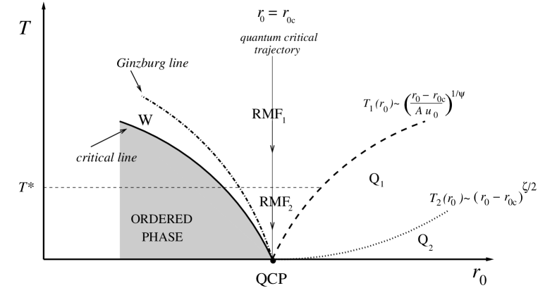
Figure 2: Qualitative global low-$T$ phase diagram for $(d\lesssim 4)$-dimensional quantum systems which emerges from our static framework. Here $T$ is the temperature and $r_{0}$ the nonthermal control parameter. The continuous line denotes the phase boundary and the noncontinuous ones indicate crossovers. The shaded region represents the ordered phase. Whitin the W region, a classical critical behavior takes place (approaching the critical line along vertical and horizontal paths). The central region is characterized by a crossover between two different regimes (${\rm RMF}_{1}$ and ${\rm RMF}_{2}$) which occurs decreasing $T$ along the quantum critical trajectory, with MF-like exponents renormalized through the shift exponent $\psi$. This is signaled by the thin dashed horizontal line $T=T^{*}$. In the region $Q_{1}$, the $T$-dependent contributions to the leading MF behavior in $(r_{0}-r_{0c})$ of relevant macroscopic quantities has a power law form again related to $\psi$. The region $Q_{2}$ corresponds to the disordered quantum regime where the thermal fluctuations are negligible. The exponent $\zeta$, which marks the crossover between the quasi-quantum regimes $Q_{1}$ and $Q_{2}$ is identified as the dynamical critical exponent $z$.

It is remarkable that the quantum critical scenario, emergent from the effective static RG treatment here performed, is quite similar to that obtained in the literature sachdev ; qpts ; sondhi ; DCqpt using RG approaches which involve directly the Matsubara-time axis.

Another key-point to be clarified is the underlying role played by the dynamical critical exponent $z$ which characterizes the intrinsic dynamics of a quantum system which exhibits a QPT. In this connection, since our theory is strictly static in nature, one may think that no direct information about the different quantum models is possible. This is not the case and information about $z$ can be simply and consistently extracted from our static results using the general feature in the theory of critical phenomena that some scaling relations exist which relate also static and dynamic exponents. Bearing this in mind, by inspection of the results collected in Table 1, it is evident that the shift exponent $\psi$ and the exponent $\zeta$, which enter in all our predictions as a manifestation of the underlying quantum degrees of freedom, are not independent but are related by

$$\zeta=\frac{d-2}{\psi-1},$$ (105)

which is valid for any quantum model considered through this paper. On the other hand, in conventional quantum RG approaches sachdev ; qpts ; sondhi ; DCqpt , when the dynamical exponent $z$ is known, for $d+z>4$ the shift exponent $\psi$ is determined in terms of $z$ through the scaling relation qpts ; millis93

$$\psi=\frac{d+z-2}{z}\;.$$ (106)

Eqs. (105) and (106), together with a careful comparison of the global static phase diagram in Fig. 2 with the corresponding ones derived by means of dynamic theories sachdev ; qpts ; millis93 , allow us to identify the exponent $\zeta$ as the appropriate dynamic exponent $z$ forthe quantum systems under study.

This identification establishes a bridge between our unified static analytical predictions and the conventional dynamic scenario. For instance, the crossover line $T_{2}(r_{0})$ in Fig. 2 can be also obtained from our leading order solution $\xi\sim(r_{0}-r_{0c})^{-1/2}$ setting (with $\zeta=z$) $\xi T^{z}\sim 1$, which coincides with that found in literature sachdev ; qpts ; sondhi ; DCqpt ; vojta-rev ; GSI ; millis93 , signaling the so-called quantum $(T\xi^{z}\ll 1)$-to-classical $(T\xi^{z}\gg 1)$ crossover. Then, when $T\ll T_{2}(r_{0})$, we are in the “disordered quantum regime” where the physics is essentially quantum in nature in the sense that the fluctuations on scale $\xi$ have energies much greater than $K_{B}T$ (where $K_{B}$ is the Boltzmann constant here assumed equal to unity).

Within this scenario, the peculiar region around the quantum critical trajectory in the phase diagram, above the crossover line $T_{1}(r_{0})$, defines the usual “quantum critical region” characterized by vertical path classical exponents renormalized as a consequence of the QCP influence.

VIII Conclusions

In summary, in this paper we have derived, within a general non-conventional framework, the low-$T$ quantum critical scenario and the crossovers induced by the interplay of thermal and quantum critical fluctuations for three wide classes of systems which exhibit a QCP, also named a “black hole” in the phase diagram modernphys . This has been performed, close to and below the classical upper critical dimensionality, by using an effective static treatment which combines a preliminary integration over degrees of freedom with non-zero Matsubara frequencies, to obtain a classical GL free energy functional with effective $T$-dependent coupling parameters, and then the genuine Wilson RG philosophy. This allowed us to extract the quantum critical properties, crossovers and the global phase diagram of the original quantum systems. In our intrinsically static RG picture, the explicit dependence of the effective coupling parameters on temperature and the original microscopic ones, played a crucial role as a result of the competition between the classical and quantum critical worlds. The emergent phase diagram was found to display all the relevant features currently obtained via more familiar approaches. Nevertheless, additional low-temperature crossovers were found as a further manifestation of the QCP influence. It is also worth emphasizing another relevant result of our static approach. As well known, the key feature which distinguishes the quantum and the most familiar finite temperature phase transitions is that, while the intrinsic dynamics of a quantum system is irrelevant for the latter, it plays a crucial role in the former. The link between statics and dynamics close to a continuous QPT is usually measured by the value of the dynamical critical exponent $z$, that describes the relative scaling of the time and the length scales in the problem. Thus, settling the value of $z$ is of a great interest, especially to distinguish different quantum universality classes. This objective is traditionally achieved using dynamic theories sachdev ; qpts ; sondhi ; DCqpt ; vojta-rev ; GSI . However, although intrinsically static, our RG analysis allowed us to obtain information about $z$ through its identification with a new exponent $\zeta$ which arises from the degrees of freedom reduction procedure as strictly related to the shift exponent $\psi$ which characterizes the low-$T$ shape of the phase boundary.

In conclusion, we hope that our simple approach may give further insight into the topical subject of QPTs and the effects of competition between thermal and quantum critical fluctuations moving in the phase diagram along appropriate thermodynamic trajectories to approach QCPs. On this matter, we believe that a relevant feature of our approach is that it allows us to work within a single parameter space in contrast with the usual one where the temperature enters explicitly the RG flows. As it is well known sachdev ; qpts ; sondhi ; DCqpt ; vojta-rev ; GSI ; noi97 ; millis93 ; noi03 ; noi05 , to extract complete physical information, the renormalization of the temperature forces to perform the rather unnatural change of the renormalized original coupling parameter $u(l)$ (see Eq. (3)) in the new one $v(l)=u(l)T(l)$ when the rescaling parameter $l$ is sensibly increased by iteration of the RG transformation. It is just this feature that implies inevitably the traditional step by step procedure and prevent, in our opinion, a unified and controllable description of the crossovers in the influence domain of a QCP. More serious problems on physical grounds emerge in the conventional RG treatments when quenched disorder is present sachdev ; revDC . We think that the key idea of our method may be usefully employed, especially in this more complex situation, for properly exploring quenched disorder effects on quantum criticality by overcoming the well known troubles sachdev ; revDC related to the Matsubara-time direction introduced by path-integral representation as an expression of the non-commutability of the operators which enter the microscopic Hamiltonian.

It is also worth mentioning that the present scenario close to the QCP, as the previous ones in literature sachdev ; qpts ; sondhi ; DCqpt ; vojta-rev ; GSI ; millis93 , is strictly valid to the one-loop approximation. Of course, corrections to the Fisher exponent $\eta$, and hence to the related ones via the usual scaling relations, are expected to higher order approximations. However, we believe that the previous physical scenario will remain qualitatively unchanged for all quantum systems of interest.

References

- (1) S. Sachdev, “Quantum Phase Transitions”, (Cambridge University Press, Cambridge 1999).
- (2) M. A. Continentino, “Quantum Scaling in Many-Body Systems” (World Scientific, Singapore, 2001).
- (3) S. L. Sondhi, S. M. Girvin, and J. P. Carini, Rev. Mod. Phys. 69, 315 (1997).
- (4) L. De Cesare and D. I. Uzunov, “Fundamental Problems on Quantum Critical Phenomena”, in “Correlation, Coherence and Order”, ed. D.V. Shopova and D.I. Uzunov (Plenum Publishers, London-New York 1999), p. 29.
- (5) T. Vojta, Ann. Phys. (Leipzig) 9, 403 (2000); M. Vojta, Rep. Progr. Phys. 66, 2069 (2003).
- (6) D. Belitz, T. R. Kirkpatrick, and T. Vojta, Rev. Mod. Phys. 77, 579 (2005).
- (7) R. B. Laughlin, G. Lonzarich, P. Monthaux, and D. Pines, Adv. Phys 50, 361 (2001); G. Chapline, E. Hohlfeld, R. B. Laughlin and D. I. Santiago, Phyl. Mag. B 81, 235 (2001); G. Chapline, Int. J. Mod. Phys. A 18, 3587 (2003); G. Chapline, astro-ph/0503200; P. Coleman and A. J. Schofield, Nature 433, 226 (2005).
- (8) H. von Löhneysen et al., Phys. Rev. Lett. 72, 3262 (1994); A. Schröder et al., Nature 407, 351 (2000).
- (9) R. S. Perry et al., Phys. Rev. Lett. 86, 2661 (2001).
- (10) C. Castellani, C. Di Castro, and M. Grilli, Z. Phys. B 103, 137 (1997); E. Dagotto, Rev. Mod. Phys. 66, 763 (1994); S. Sachdev, Science 288, 475 (2000).
- (11) J. Hertz, Phys. Rev. B 14, 1165 (1976).
- (12) A. P. Young, J. Phys. C: Solid State Phys. 8, L309 (1975); P. Pfeuty, J. Phys. C: Solid State Phys. 9, 3993 (1976), and reference therein.
- (13) P. R. Gerber and H. Beck, J. Phys. C: Solid State Phys. 10, 4013 (1977).
- (14) I. D. Lawrie, J. Phys. C: Solid State Phys. 11, 3857 (1978).
- (15) L. De Cesare, Lett. Nuovo Cim. 22, 325, 632 (1978); G. Busiello and L. De Cesare, Nuovo Cim. 59, 327 (1980); J. Phys. A: Math. Gen., 13, 3779 (1980); Phys. Lett. A 77, 177 (1980).
- (16) I. Goldhirch, J. Phys. C: Solid State Phys.12, 5345 (1979).
- (17) G. Busiello, L. De Cesare, and I. Rabuffo, Physica A 117, 445 (1983), and references therein.
- (18) R. Micnas and K. A. Chao, Phys. Lett. A 110, 269 (1985).
- (19) A. Caramico D’Auria, L. De Cesare, and I. Rabuffo, Physica A 243, 152 (1997), and references therein.
- (20) As concerning the exactly solvable classical model with see: R. Bolian and G. Toulouse, Phys. Rev. Lett. 30, 544 (1973); P. Pfeuty and G. Toulouse, “Introduction to the Renormalization Group and to Critical Phenomena”, (John Wiley & Sons, London, 1977), Ch. 2 Sec. 2.6.
- (21) D. I. Uzunov, Phys. Lett. 87 A, 11 (1981).
- (22) T. K. Kopec and G. Koslowskí, Phys. Lett. 95 A, 104 (1983); A. V. Chubukov, Theor. Math. Phys. 60, 728 (1985).
- (23) L. De Cesare, Nuovo Cim. D 1, 289 (1982).
- (24) Y. Baba, T. Nagai, and K. Kawasaki, J. Low Temp. Phys. 36, 1 (1979).
- (25) D. Schmeltzer, Phys. Rev. B 28, 459 (1983); ibidem 29, 2815 (1984); 32, 7512 (1985).
- (26) K. Walasek, Phys. Lett. A 101, 343 (1983); K. Lukierska-Walasek, Physica A 127, 613 (1984); K. Lukierska-Walasek and W. Salejda, Phys. Lett. A 111, 415 (1985).
- (27) M. Rasolt, M. J. Stephen, M. E. Fisher, and P. B. Weichman, Phys. Rev. Lett. 53, 798 (1984); D. S. Fisher and P. C. Hohenberg, Phys. Rev. B 37, 4936 (1988); S. Chakravarty, B. I. Halperin, and D. R. Nelson, Phys. Rev. B 39, 2344 (1989); S. Sachdev and J. Ye, Phys. Rev. Lett 69, 2411 (1992); A. Sokol and D. Pines, Phys. Rev. Lett. 71, 2813 (1993).
- (28) A. J. Millis, Phys. Rev. B 48, 7183 (1993).
- (29) S. Sachdev, A. V. Chubukov, and A. Sokol, Phys. Rev. B 51 14874 (1995); A. M. Sengupta and A. Georges, Phys. Rev. B 52, 10295 (1995); S. Sachdev and E. R. Dunkel, Phys. Rev. B 73, 085116 (2006).
- (30) A. Caramico D’Auria, L. De Cesare, and I. Rabuffo, Physica A 327, 442 (2003).
- (31) A. Caramico D’Auria, L. De Cesare, M. T. Mercaldo, and I. Rabuffo, Physica A 351, 294 (2005).
- (32) R. Oppermann and H. Thomas, Z. Physik B 22, 387 (1975); T. Schneider, H. Beck, and E. Stoll, Phys. Rev. B 13, 1123 (1976); R. Morf, T. Schneider, and E. Stoll Phys. Rev. B 16, 462 (1977); I. D. Lawrie, J. Phys. C: Solid State Phys. 11, 1123 (1978); P. R. Gerber, J. Phys. C: Solid State Phys. 11, 5005 (1978).
- (33) K. Walasek, Physica A 137, 258 (1986).
- (34) T. Vojta, Phys. Rev. B 53, 710 (1996).
- (35) S. Sachdev, Phys. Rev. B 55, 142 (1997).
- (36) J. Rudnick and D. R. Nelson, Phys. Rev. B 13, 2208 (1976).
- (37) B.K. Chakrabarti, A. Dutta, P. Sen, “Quantum Ising Phases and transitions in Transverse Ising Model”, Springer, Berlin (1996).
- (38) N. Kawashima, J. Phys. Soc. Jpn. 74, 145 (2005); E. Dagotto, Rep. Progr. Phys 62, 1525 (1999).
- (39) Q. Si, S. Rabello, K. Ingersent and J. L. Smith, Nature 413, 804 (2001); A. Abanov and A. V. Chubukov, Phys. Rev. Lett. 93, 255702 (2004).
- (40) D. Belitz and T. R. Kirkpatrick , Phys. Rev. Lett. 89, 247202 (2002); D. Belitz, T. R. Kirkpatrick, and T. Vojta, Phys. Rev. B 65, 165112 (2002); T. R. Kirkpatrick and D. Belitz Phys. Rev. B 67, 024419 (2003); for disordered systems: D. Belitz, T. R. Kirkpatrick, M. T. Mercaldo, and S. L. Sessions, Phys. Rev. B 63, 174427 (2001), Phys. Rev. B 63, 174427 (2001); for a review see GSI .
- (41) A. V. Chubukov, C. Pepin and J.Rech, Phys. Rev. Lett. 92,147003 (2004); J. Rech, C. Pepin and A. V. Chubukov, cond-mat/0605306.
- (42) The index in the exponents signals that the critical line is approached by variation of the non-thermal control parameter at fixed . A different index () will be used when vertical paths are used, i.e. trajectories parallel to the -axis in the phase diagram.
- (43) U. T. Höchli and L. A. Boatmer, Phys. Rev. B 20, 266 (1979); D. Rytz, U. T. Höchli, and H. Bilz, Phys. Rev. B 22, 359 (1980); K.A. Müller, Japan J. Appl. Phys. 24 (Suppl. 2), 89 (1985).
- (44) G.A. Samara, Physica B 150, 179 (1988), and references therein.
- (45) W. A. C. Erkelens, L. P. Regnault, J. Rossat-Mignod, J. E. Moore, R. A. Butera, L. J. De Jongh, Europhys. Lett. 1, 37 (1986); D. Bitko, T. F. Rosenbaum, and G. Aeppli, Phys. Rev. Lett. 77, 940 (1996).
- (46) L. De Cesare, Rev. Solid State Sci. 3, 71 (1989).