Ostwald ripening of faceted two-dimensional islands

Abstract

We study Ostwald ripening of two-dimensional adatom and advacancy islands on a crystal surface by means of kinetic Monte Carlo simulations. At large bond energies the islands are square-shaped, which qualitatively changes the coarsening kinetics. The Gibbs–Thomson chemical potential is violated: the coarsening proceeds through a sequence of ‘magic’ sizes corresponding to square or rectangular islands. The coarsening becomes attachment-limited, but Wagner’s asymptotic law is reached after a very long transient time. The unusual coarsening kinetics obtained in Monte Carlo simulations are well described by the Becker–Döring equations of nucleation kinetics. These equations can be applied to a wide range of coarsening problems.

I Introduction

Domains of a guest phase inside a matrix tend to coarsen, thus reducing their specific interface energy. The prominent mechanism of coarsening was proposed by OstwaldOstwald (1900) more than hundred years ago: larger domains grow at the expense of smaller ones by exchanging atoms. The net atom flux is directed to larger domains since they possess smaller interface energy per atom. The seminal theory of Ostwald ripening was proposed by Lifshitz and SlyozovLifshitz and Slyozov (1961) and by Wagner.Wagner (1961) They showed that, at late times, the system is characterized by a single characteristic scale, namely, the average domain size $R(t)$. The time evolution of the system consists in changing the scale: the domain distribution, shape of the diffraction peaks, etc. remain unchanged when scaled by $R(t)$. The average domain size follows, in turn, universal laws, $R(t)\propto t^{1/3}$ if the atom diffusion is the rate limiting processLifshitz and Slyozov (1961) and $R(t)\propto t^{1/2}$ if the attachment-detachment at the domain interface is the limiting one.Wagner (1961)

The kinetic scaling is essentially based on the Gibbs–Thomson formula $\mu=\gamma/R$ for the excess chemical potential of a gas that is in equilibrium at the curved surface of a liquid droplet (the constant $\gamma$ is proportional to the surface tension). The aim of the present work is to study the Ostwald ripening kinetics at low temperatures (or large bond energies) when the crystalline droplets are faceted. The energy of a small crystalline droplet is minimum at ‘magic’ sizes when all facets are completed. The coarsening proceeds as a sequence of jumps from one magic size to the next. We perform kinetic Monte Carlo simulations of Ostwald ripening kinetics for faceted two-dimensional (2D) islands and find very long transient behavior of the system, so that the universal asymptotic laws are still not reached. We develop a mean-field theory for Ostwald ripening, based on the Becker–DöringBecker and Döring (1935) equations. We show that these equations, being the basic equations of nucleation theory,Frenkel (1946); Lewis and Anderson (1978) can be used to describe the coarsening kinetics in the whole size range, starting from monomers up to the long-time asymptotics that are not available in Monte Carlo simulations. Both the Lifshitz–Slyozov–Wagner regime and the coarsening through a sequence of magic sizes are well described. This approach requires only the knowledge of the droplet energy dependence on the number of atoms in the droplet and can be applied to a wide range of coarsening problems in other systems as well.

Two-dimensional (2D) islands on a crystal surface are a practically important physical system that reveals different coarsening mechanisms and allows detailed theoretical and experimental studies of the coarsening kinetics. From the experimental studies, we mention the ones that report time exponents $n$ in the coarsening law $R(t)\propto t^{n}$. These include low-energy electron diffraction from a chemisorbed monolayer of oxygen on W(110),Tringides et al. (1987); Wu et al. (1989) helium atom beam diffraction from 0.5 monolayer (ML) of Cu on Cu(100),Ernst et al. (1992) optical microscopy of a thin layer of succinonitrile within the liquid-solid coexistence regionKrichevsky and Stavans (1993, 1995) and a binary mixture of amphiphilic molecules,Seul et al. (1994) and low-energy electron microscopy of Si on Si(001).Theis et al. (1995); Bartelt et al. (1996) In these works,Tringides et al. (1987); Wu et al. (1989); Ernst et al. (1992); Krichevsky and Stavans (1993, 1995); Seul et al. (1994) the time exponents somewhat smaller than $1/3$ were found and explained by the Lifshitz–Slyozov law with finite-size corrections. The time exponent $1/2$ obtained for Si on Si(001)Theis et al. (1995); Bartelt et al. (1996) was treated as the case of kinetics limited by the attachment and detachment of adatoms to steps.Wagner (1961) Our recent x-ray diffraction study of coarsening of 2D GaAs islands on GaAs(001),Braun et al. (2004) which showed an apparent time exponent close to 1, was the experimental inspiration for the present work.

Two-dimensional islands of ‘magic’ sizes were observed on several surfaces, such as Pt(111)Rosenfeld et al. (1992), Si(111),Voigtländer et al. (1998) and Ag(111)Morgenstern et al. (2005) (see also a reviewWang and Lai (2001)). It was shown theoretically that the presence of magic island sizes disrupts the scaling law of submonolayer molecular beam epitaxy growth.Schroeder and Wolf (1995) Magic sizes of three-dimensional Pb nanocrystals on Si(111) lead to a breakdown of the classical Ostwald ripening laws.Jeffrey et al. (2006)

Monte Carlo simulations of Ostwald ripening were performed using the 2D Ising model.Huse (1986); Amar et al. (1988); Roland and Grant (1989) They were limited to rather small values of the coupling constant, so that the domains are rounded and faceting is absent. The time exponents were found to be smaller than $1/3$, which was explained by finite-size corrections to the Lifshitz–Slyozov law. Further discussion of theoretical and simulation studies can be found in several reviews.Voorhees (1985); Mouritsen (1990); Bray (1994) Despite kinetic Monte Carlo simulations are routinely used to model epitaxial growth,Clarke and Vvedensky (1987, 1988); Clarke et al. (1989, 1991); Shitara et al. (1992a, b) we are aware of only one such study of coarsening of 2D islands on a crystal surface.Lam et al. (1999) This latter simulation was limited to small bond energies and rounded islands, similar to the simulations of the Ising model.

A physical difference between the coarsening kinetics of 2D epitaxial islands and that of Ising spins becomes evident when we compare adatoms and advacancies on one side with up and down spins on the other side. The first two objects possess qualitatively different kinetics (motion of an advacancy is a result of the collective motion of atoms), while up and down spins are equivalent. This distinction manifests itself in the transition probabilities, as discussed below. The fundamental laws of Ostwald ripening are expected to be independent of the transition probability distribution, so that a kinetic Monte Carlo simulation of the coarsening of epitaxial islands allows one to check this conclusion. Here, we perform kinetic Monte Carlo simulations of Ostwald ripening of 2D adatom islands (surface coverage 0.1 ML) and 2D advacancy islands (surface coverage 0.9 ML) in a wide range of bond energies (or temperatures). Our particular aim is to perform simulations in the case of large bond energies (low temperatures) when the islands are faceted, which was not studied previously.

II Monte Carlo simulations

II.1 Simulation method

We employ the well-established generic model developed for kinetic Monte Carlo simulations of molecular beam epitaxy.Clarke and Vvedensky (1987, 1988); Clarke et al. (1989, 1991); Shitara et al. (1992a, b); Lam et al. (1999) Atoms occupy a simple cubic lattice and interact with a pair energy that depends only on the number of bonds. An alternative approach to simulate surface kinetics is a detailed Monte Carlo simulation of a particular surface with energetic parameters taken from ab initio calculations, as it was done for GaAs(001) or InAs(001).Kratzer et al. (1999); Kratzer and Scheffler (2002); Grosse et al. (2002a); Grosse and Gyure (2002); Grosse et al. (2002b) Such simulations are very time-consuming and hence are limited to small time and spatial scales. They can hardly be applied to study the coarsening process. Some characteristic features of compound semiconductors can, however, be included in the generic model as a compromise.Heyn and Harsdorff (1997); Heyn et al. (1997); Zhang and Orr (2003)

We use an algorithmBortz et al. (1975) that advances simulated time depending on the probability of the chosen event. This algorithm is commonly used in the epitaxial growth simulations. We note that the Ostwald ripening simulations of the 2D Ising modelHuse (1986); Amar et al. (1988); Roland and Grant (1989) have employed the Metropolis accept–reject algorithm. This algorithm becomes ineffective at low temperatures, since most of the attempts are rejected and computer time is wasted. That is why previous simulationsHuse (1986); Amar et al. (1988); Roland and Grant (1989) were restricted to relatively high temperatures $T>0.5T_{c}$, where $T_{c}$ is the Ising phase transition temperature. Of course, both algorithms give the same results and differ only in the computation time.

The choice of the probability $w(\mathbf{x}\rightarrow\mathbf{y})$ for the transition from the state $\mathbf{x}$ to the state $\mathbf{y}$ incorporates the physics of the system into the simulations. The choice is made differently for the epitaxial growth and the Ising model simulations. It is worthwhile to compare these probabilites briefly. A sufficient condition that the system evolves to thermodynamic equilibrium is the detailed balance condition, $w(\mathbf{x}\rightarrow\mathbf{y})/w(\mathbf{y}\rightarrow\mathbf{x})=\exp(-\Delta E/k_{\mathrm{B}}T)$. Here $\Delta E=E(\mathbf{y})-E(\mathbf{x})$ is the energy difference between the states $\mathbf{x}$ and $\mathbf{y}$, $k_{\mathrm{B}}$ is the Boltzmann constant and $T$ is the temperature. The simulations of the Ising model use a probability that depends on $\Delta E$ (either the Metropolis or the Glauber probability). These probabilities favor transitions which reduce the energy of the system, $\Delta E<0$. On the other hand, for an atom jump on the crystal surface, the transition probability does not depend on the final state $\mathbf{y}$ but only on the height of the energy barrier that needs to be overcome.Kang and Weinberg (1989) The probability is $w(\mathbf{x}\rightarrow\mathbf{y})\propto\exp[E(\mathbf{x})/k_{\mathrm{B}}T]$, where $E(\mathbf{x})<0$ is the energy of the initial state with respect to the barrier. Such a probability obviously satisfies the detailed balance condition. The system evolves into a lower-energy state since it escapes higher-energy initial states with larger probabilities.

In the present study, no step edge barrier is imposed. An atom detaching from a step edge can go to the lower or the upper terrace with equal probabilities. In particular, atom exchange between advacancy islands is achieved predominantly by adatoms diffusing on the top level rather than by the diffusion of vacancies, despite that the latter process is not forbidden. Similar simulations, but with an infinite step edge barrier, were performed in our preceding work.Kaganer et al. (2006) In that study, the restriction for atoms to escape a vacancy island to the higher level resulted in another coarsening mechanism, diffusion and coalescence of whole islands due to atom detachment and reattachment within an island. The coarsening by dynamic coalescence is much less effective than Ostwald ripening and becomes essential when the detachment of atoms form islands is prohibited.

An atom that has $n$ neighbors in the initial state with equal bond energies $E_{b}$ to these neighbors, possesses an energy $E(\mathbf{x})=-(nE_{b}+E_{D})$, where the activation energy of surface diffusion $E_{D}$ is the barrier height. It determines the time scale $\tau$ of the problem, $\tau^{-1}=\nu\exp(-E_{D}/k_{\mathrm{B}}T)$, where $\nu\approx 10^{13}$ s^-1 is the vibrational frequency of atoms in a crystal. In the epitaxial growth simulations, the time scale $\tau$ is to be compared with the deposition flux, which determines an appropriate choice of $E_{D}$. We do not consider deposition, and the choice of $E_{D}$ is arbitrary. Note that the works on the Ising model kinetics measure time simply in the flip attempts (sweeps) per lattice site. We take the same values of $E_{D}$ as in the preceding work,Kaganer et al. (2006) with the aim to compare time scales of Ostwald ripening (in absence of the step edge barrier) with that of dynamic coalescence (infinite step edge barrier). Namely, we take $E_{D}=0.2$; $0.1$; $0$ eV for $E_{b}=0.2$; $0.3$; $0.4$ eV, respectively.

The ratio of the interaction energy between neighboring atoms to the temperature $E_{b}/k_{\mathrm{B}}T$ is the only essential parameter for the coarsening problem. We fix the temperature at 400 K and vary the bond energy $E_{b}$ from 0.2 eV to 0.4 eV. In terms of our model, the Ising phase transition takes place at $E_{b}/k_{\mathrm{B}}T=2\ln(1+\sqrt{2})$. Our choice of bond energies corresponds to $T/T_{c}$ varying from 0.15 to 0.3, temperatures much lower than the ones used in previous kinetic Monte Carlo studies of Ostwald ripening.Huse (1986); Amar et al. (1988); Roland and Grant (1989); Lam et al. (1999) Here $T_{c}$ is the Ising phase transition temperature.

We perform kinetic Monte Carlo simulations on a 1000$\times$1000 square grid with periodic boundary conditions. Each simulation is repeated 25 times, to obtain sufficient statistics for the island size distribution. In the initial state, either 0.1 ML or 0.9 ML are randomly deposited. Adatom islands form in the first case and advacancy islands in the second.

II.2 Simulation results

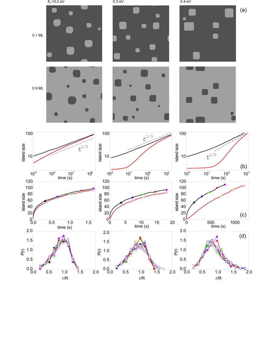
Figure 1: Results of kinetic Monte Carlo simulations: (a) snapshots of the 1000$\times$1000 simulation cells at the end of the simulations, (b) and (c) time dependence of the average island size in logarithmic and linear scales, and (d) the island size distributions. The gray levels in the snapshots vary from black to white as the surface height increases. Different columns show results for different bond energies $E_{b}$, with the temperature fixed at $T=400$ K. The size distributions are obtained at the time moments marked in (c) by the corresponding symbols.

Snapshots of the simulated system at the end of a simulation are presented in Fig. 1(a). As the bond energy $E_{b}$ is increased (from left to right), the island shape continuously transforms from more circular to almost square. Since faceting transitions are absent in 2D systems, we refer to the almost square islands as faceted in order to stress the qualitative shape difference at small and large bond energies. Apart from the change in shape, the equilibrium density of adatoms between islands exponentially decreases as the bond energy increases.

Figures 1(b) and (c) show time variations of average island diameters $2R(t)$ in logarithmic and linear scales, respectively. The determination of an average island size is described in Sec. II.3. At small bond energies (left column in Fig. 1), the process of Ostwald ripening follows the Lifshitz–Slyozov law $R(t)\propto t^{1/3}$. As the bond energy increases, the coarsening law for advacancy islands deviates from that for adatom islands and from the expected $t^{1/3}$ law. At large bond energies (right column in Fig. 1), the coarsening behavior of advacancy islands is qualitatively different and close to a linear dependence, in a wide range of island sizes. The coarsening of adatom islands also notably deviates from the Lifshitz–Slyozov law. The attachment-limited asymptotic $t^{1/2}$ can be inferred from the figure, but it is not really reached.

Figure 1(d) shows the island size distributions at different times. The uniformly spaced time instances are marked on the curves in Fig. 1(c) by the same symbols as used for the corresponding size distributions. The distributions are scaled by the average size $R(t)$: instead of the probability $P(r)$, we plot $RP(r)$ versus $r/R$. The scaled distributions do not change in time even at large bond energies, where the average island sizes do not show a power law behavior. The island size distribution notably changes with increasing bond energy, Fig. 1(d). The distribution develops a tail extended to $2R$, while at smaller bond energies it is limited to $1.5R$.

II.3 Analysis of the simulation data

We obtain the sizes of all islands in the simulated system by using an algorithmHoshen and Kopelman (1976) that allows to count all topologically connected clusters in the system. At large bond energies, we average the radii $r_{n}=\sqrt{n/\pi}$ (where $n$ is the number of atoms in a cluster) of all islands, excluding individual adatoms from the distribution. In the case of small bond energies we find that, besides monomers, a notable amounts of transient dimers, trimers, etc. are present in the simulated system. Their densities quickly decrease with increasing number of atoms in the cluster and they are well separated from the distribution of the large clusters. If these small clusters are included in the island size distribution when calculating average radius $R$, we obtain unreasonable time dependencies $R(t)$. Hence, we calculate the averages taking into account islands of at least 6 atoms.

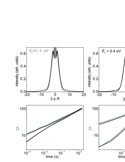
Figure 2: (a) Diffraction peaks obtained from the Monte Carlo simulation results (the gray curves are Gaussian fits). (b) Time dependencies of the average island sizes obtained from the numbers of atoms in the clusters (black curves) and from the widths of the diffraction peaks (gray curves).

We also use the Monte Carlo simulations to verify the average island size determination in diffraction studies. In a diffraction experiment, one has access to the peak profile only and obtains the average size from its width. Using the island distribution obtained in the simulation and calculating the peak profiles, we can compare the average sizes obtained from the real space and the reciprocal space distributions. The diffraction peaks (structure factors) obtained from the simulations are present in Fig. 2(a). We consider the anti-Bragg condition (subsequent atomic layers contribute to the scattering function with a phase shift of $\pi$) and obtain two-dimensional intensity distributions $I(q_{x},q_{y})$ from Fourier transformation of $\exp[i\pi h(x,y)]$. Here an integer function $h(x,y)$ is the surface height. Then, we take into account that in a diffraction experiment, the scattered intensity is usually collected by a wide open detector that integrates over one of the components of the scattering vector $\mathbf{q}$.Braun et al. (2004) Hence, we integrate the distributions $I(q_{x},q_{y})$ over one of the components of the scattering vector, either $q_{x}$ or $q_{y}$. The resulting diffraction peaks $I(q)$ are presented in Fig. 2(a). The peaks corresponding to different time moments [the same time moments as in Fig. 1(d)] coincide after the wave vectors $q$ are scaled by the average island size. Kinetic scaling is thus confirmed. The shapes of the peaks depend on the bond energy $E_{b}$, thus showing that the island size distribution and the correlations between islands change.

The quantity most commonly measured in a diffraction experiment is the full width at half maximum (FWHM) of a peak obtained by an appropriate fit. Considering islands of linear size $2R$, one obtains a structure factor $\sin^{2}(qR)/\sin^{2}(qa)$, which can be approximated by $\exp(-q^{2}R^{2}/\pi)$.Warren (1969) Here, $a$ is the lattice spacing. We obtain the average size $2R$ by fitting the peaks to this Gaussian function, despite the peaks are not Gaussian, especially for small bond energies. Figure 2(b) compares these sizes with the ones obtained from the real-space island size analysis described above. The values are in good agreement, thus confirming that the average quantities can be obtained from the diffraction peak widths even if the profiles deviate notably from Gaussian.

III Coarsening equations

III.1 The Becker–Döring equations for the 3D problem

The process of Ostwald ripening can be described by two alternative approaches, either in terms of a continuous function $f(r)$ representing the number density of clusters of radius $r$, or in terms of discrete numbers $c_{n}$ representing the densities of clusters containing $n$ atoms ($n$mers). The first approach was employed by Lifshitz and SlyozovLifshitz and Slyozov (1961) and Wagner.Wagner (1961) The equations for discrete quantities $c_{n}$ were first formulated by Becker and DöringBecker and Döring (1935) and ever since form the basis of nucleation theory.Frenkel (1946); Lewis and Anderson (1978) Closely related equations, the rate equations, were used in the description of crystal growth.Zinsmeister (1966); Stoyanov and Kaschiev (1981); Venables et al. (194) They contain an additional deposition term, while the detachment process is not essential and the corresponding terms in the equations are frequently omitted. Similar discrete equations for the Ostwald ripening process were introduced under the names of microscopic continuity equations,Dadyburjor and Ruckenstein (1977); Bhakta and Ruckenstein (1995) population balance equations, Madras and McCoy (2002, 2003, 2005) or rate equation approach.Xia and Zinke-Allmang (1998) Mathematical aspects of the relationship between the discrete and the continuous equations were also considered.Penrose (1997); Collet et al. (2002) The aim of the present section is to link the discrete and continuous approaches and obtain equations that can be used for a numerical study of the Ostwald ripening process.

The number of atoms $n$ in a cluster increases or decreases by one when an atom is attached to the cluster or detached from it. Let $J_{n}$ be the net rate of transformation of $n$mers into $(n+1)$mers. The number $c_{n}$ of $n$mers increases due to the transformation of $(n-1)$mers into $n$mers and decreases because of the transformation of $n$mers into $(n+1)$mers:

$$dc_{n}/dt=J_{n-1}-J_{n}.$$ (1)

This equation is valid for $n\geq 2$. The equation describing the number of monomers $c_{1}$ is obtained by requiring that the total number of atoms in the system

$$N=\sum_{n=1}^{\infty}nc_{n}$$ (2)

does not change in time. The condition $dN/dt=0$ gives, after substitution of Eqs. (1) and rearrangement of the terms,

$$dc_{1}/dt=-2J_{1}-\sum_{n=2}^{\infty}J_{n}.$$ (3)

This equation takes into account that each transformation of an $n$mer into an $(n+1)$mer decreases the number of monomers by one, except in the case $n=1$, where two monomers form a dimer.

The net rate $J_{n}$ is a result of two processes. First, an $n$mer catches a monomer. The rate of this process is proportional to the densities of the $n$mers and the monomers and can be written as $a_{n}c_{1}c_{n}$, where $a_{n}$ is a time-independent coefficient that remains to be determined. The second process is a spontaneous detachment of a monomer from a $(n+1)$mer. It is proportional to the density of $(n+1)$mers solely and can be written as $b_{n}c_{n+1}$, where $b_{n}$ is another time-independent coefficient to be specified. Hence, we obtain

$$J_{n}=a_{n}c_{1}c_{n}-b_{n}c_{n+1}.$$ (4)

Equations (1), (3), and (4) are the Becker–Döring equations.

If the time limiting process is the adatom diffusion between clusters, the attachment and detachment coefficients $a_{n}$ and $b_{n}$ for the 3D problem are calculated, for large $n,$ as follows. The cluster of $n$ atoms is considered as a sphere of radius $r_{n}$, so that $n=4\pi r_{n}^{3}/3$. To calculate the attachment coefficient, we solve the steady-state diffusion equation $\nabla^{2}c(r)=0$ with two boundary conditions: the concentration of the monomers far away from the cluster is equal to their mean concentration, $c(r)\left|{}_{r=\infty}\right.=c_{1}$, while the concentration of the monomers at the cluster surface is zero, $c(r)\left|{}_{r=r_{n}}\right.=0$, since the monomers are attached to the cluster as soon as they reach it. The solution is $c(r)=(1-r_{n}/r)c_{1}$. The total atom flux at the cluster surface

$$j_{n}=4\pi r_{n}^{2}D\nabla c(r)\left|{}_{r=r_{n}}\right.,$$ (5)

where $D$ is the diffusion coefficient of the monomers, is equal to $4\pi Dr_{n}c_{1}$, and hence the attachment coefficient is

$$a_{n}=4\pi Dr_{n}.$$ (6)

The detachment coefficient is calculated assuming that the concentration of the monomers at the cluster surface is equal to the equilibrium monomer concentration $c_{n\mathrm{eq}}$, while there is an ideal sink for monomers at infinity, $c(r)\left|{}_{r=\infty}\right.=0$. The solution of the steady-state diffusion equation with these boundary conditions is $c(r)=c_{n\mathrm{eq}}r_{n}/r$, and the corresponding detachment flux of the monomers is $b_{n+1}=4\pi Dr_{n}c_{n\mathrm{eq}}$. Here we take into account that this flux refers to the detachment from the $(n+1)$mer. The ratio of the detachment and the attachment coefficients is then

$$b_{n+1}/a_{n}=c_{n\mathrm{eq}}.$$ (7)

The equilibrium density of monomers at the surface of a cluster is given by the Gibbs–Thomson formula

$$c_{n\mathrm{eq}}=c_{\infty\mathrm{eq}}\exp(\gamma/r_{n})\approx c_{\infty\mathrm{eq}}(1+\gamma/r_{n}),$$ (8)

where $\gamma$ is a constant proportional to the surface tension. The explicit expression for $\gamma$ is given in the next section. A correction to Eq. (8) for small clusters consisting of very few atoms, that is important in the theory of nucleation, is not essential for the Ostwald ripening problem. Then, equations (1)–(8) give a complete set of equations that describe the process of Ostwald ripening.

When clusters are large enough, $n$ can be treated as a continuous variable. Let us verify that the continuous equations derived from the set of equations above are the Lifshitz–Slyozov equations. The cluster size distribution function $f(r,t)$ is defined so that $f(r,t)dr$ is the number of clusters per unit volume in an interval from $r$ to $r+dr$. Then, $f(r,t)dr=c_{n}(t)dn$ and, keeping in mind that $n=4\pi r^{3}/3$, we obtain $f(r,t)=4\pi r^{2}c_{n}(t)$. The mass conservation law (2) can be rewritten, by separating monomers and larger clusters, as

$$c_{1}(t)+\frac{4\pi}{3}\int_{0}^{\infty}r^{3}f(r,t)dr=N=\mathrm{const}.$$ (9)

The finite-difference equation (1) transforms into the continuity equation

$$\partial f/dt+\partial J/\partial r=0.$$ (10)

To calculate the flux in the cluster size space $J(r,t)$, one can neglect the difference between $c_{n}$ and $c_{n+1}$ in Eq. (4). Then, substituting Eqs. (7) and (8), one obtains

$$J(r,t)=\frac{D}{r}(c_{1}-c_{\infty\mathrm{eq}}-\frac{\gamma c_{\infty\mathrm{eq}}}{r})f.$$ (11)

Equations (9)–(11) coincide with the Lifshitz–Slyozov equations.Lifshitz and Slyozov (1961)

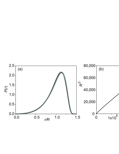
Figure 3: (a) The cluster size distribution obtained by numerical solution of the Becker–Döring equations at different times (thin black lines, the lines closer to the gray line correspond to later times) and the analytical solution by Lifshitz and Slyozov (thick gray line). (b) The time dependency of $R^{3}$. A linear asymptotic is evident from the plot.

As an example, we compare in Fig. 3 numerical solutions of the ordinary differential equations (1)–(8) with the analytical result.Lifshitz and Slyozov (1961) To solve the Becker–Döring system, we employ a second-order Rosenbrock method, which is essentially based on a Pade-approximation of the transition operator (see, e.g., Ref. Hairer and Wanner, 2004). A version of this methodLevykin and Novikov (1996) that fits well to stiff systems of differential-algebraic equations was used. Practically, we solve a set of up to one million ordinary differential equations on a personal computer. The solutions in Fig. 3 are obtained by taking $\gamma=5$ and, as the initial condition at $t=0,$ only monomers with the initial supersaturation $c_{1}/c_{\infty\mathrm{eq}}=10^{5}$. The figure shows that the numerical solutions asymptotically converge to the analytical formula, which validates our approach.

III.2 Attachment and detachment coefficients

Equation (7) can be derived in a more general form that will be useful for the considerations below. In equilibrium, all fluxes $J_{n}$ are identically equal to zero. Then, denoting by $C_{n}$ the equilibrium concentrations of the $n$mers, we have from Eq. (4)

$$b_{n+1}/a_{n}=C_{1}C_{n}/C_{n+1}.$$ (12)

The equilibrium concentrations calculated in the framework of equilibrium thermodynamics areWalton (1962)

$$C_{n}=C_{1}^{n}\exp[-(E_{n}-nE_{1})/k_{\mathrm{B}}T],$$ (13)

where $E_{n}$ is the energy of an $n$mer and $E_{1}$ is the energy of a monomer. This relation can be treated as the mass action law for the equilibrium between $n$mers and monomers, $C_{n}\leftrightarrows nC_{1}$. Substitution into Eq. (12) gives

$$b_{n+1}/a_{n}=c_{\infty\mathrm{eq}}\exp[(E_{n+1}-E_{n})/k_{\mathrm{B}}T],$$ (14)

where $c_{\infty\mathrm{eq}}=\exp(-E_{1}/kT)$ is the concentration of monomers that are in equilibrium with an infinite cluster. For spherical clusters, Eq. (14) reduces to the Gibbs–Thomson formula. The energy of a spherical cluster is $E_{n}=4\pi r^{2}\sigma$, where $\sigma$ is the surface tension, with the radius $r$ defined by $nv=4\pi r^{3}/3$, where $v=a^{3}$ is the volume per atom. The radius increase due to the attachment of an atom to a $n$mer is given by $v=4\pi r^{2}\Delta r$. The change of the energy due to the attachment of a single atom is $E_{n+1}-E_{n}=8\pi\sigma r\Delta r=2v\sigma/r$. Thus, we arrive at Eq. (8) with $\gamma=2v\sigma/k_{\mathrm{B}}T$. A similar calculation for the 2D case gives $\gamma=s\sigma/k_{\mathrm{B}}T$, where $s$ is the area per atom.

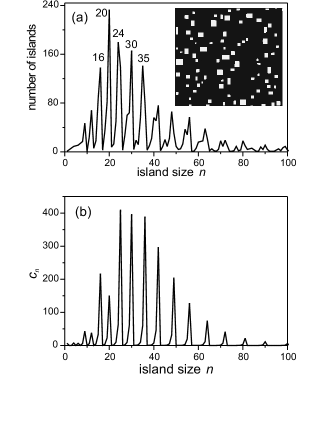
Figure 4: The island size distribution of faceted islands obtained in the kinetic Monte Carlo simulations (a) and by numerical solution of the Becker–Döring equations (b). The strong preference of magic island sizes is obvious.

Equation (14) is more general than the Gibbs–Thomson formula and can be used in situations when the latter is not applicable. Figure 4(a) presents the island size distribution obtained in our kinetic Monte Carlo simulations at an early stage of coarsening for the largest bond energy we have studied, $E_{b}=0.4$ eV. The distribution is not smooth but consists of peaks at ‘magic’ island sizes corresponding to a product of two close integers, like $30=6\times 5$. Accordingly, the insert in the figure shows that the islands are mainly rectangles with an aspect ratio close to 1. The origin of such a distribution is evident: when an island consisting, for example, of 30 atoms, grows by one atom, its energy increases by $2E_{b}$, while further growth to 36 atoms does not change its energy at all. Thus, we solve the Becker–Döring equations with the energy of a 2D island of $n$ atoms calculated as follows. First, we find the largest square that still contains fewer atoms than $n$. Then, we add, as long as the number of atoms does not exceed $n$, rows of atoms to the side of the square. The last row may be incomplete. The number of broken bonds for such an island is calculated. Figure 4(b) presents a numerical solution of the Becker–Döring equations with the island energies $E_{n}$ thus calculated and the attachment–detachment coefficient ratio given by Eq. (14). The approximation for $a_{n}$ appropriate for the 2D case is given below in Sec. III.3. The size distribution closely reproduces the one obtained in the Monte Carlo simulations: squared or rectangular (with aspect ratio close to 1) islands are discrete barriers to be overcome, while the filling of an atomic row does not change the island energy and proceeds relatively fast. This example shows that Eq. (14) can be used when the island energy $E_{n}$ is known but is not described simply by the surface tension, and the Gibbs–Thomson formula is not applicable.

III.3 Coarsening equations in two dimensions

The Becker–Döring equations (1)–(4) and the equation (14) for the ratio of the coefficients $b_{n+1}/a_{n}$ do not depend on the dimensionality of the system and can be applied to both 2D and 3D problems. (It may be worth to note that the radius $r_{n}$ entering the Gibbs–Thomson law is expressed differently through $n$ in the 2D and 3D cases.) The only formula that has to be reconsidered is expression (6) for the attachment coefficients $a_{n}$, since it is based on the solution of the 3D diffusion equation. The solution of the 2D diffusion equation behaves as $c(r)\propto\ln r$ and the boundary condition $c(r)\left|{}_{r=\infty}\right.=c_{1}$ cannot be imposed. A simple approximation is to place this condition at a finite distance $l$, given by an average distance between the islands.Chakraverty (1967); Rogers and Desai (1989); Ardell (1990); Bhakta and Ruckenstein (1995); F. Haußer and Voigt (2005) Then, in the case of diffusion-limited kinetics, the attachment coefficient $a_{n}$ does not depend on $n$ and is proportional to $(\ln l)^{-1}$. Proceeding to the continuous distribution function, one arrives at Eq. (11), with the conservation law (9) rewritten for the 2D case. The coarsening equations are solved analytically in this case.Hillert (1965); Rogers and Desai (1989); Ardell (1990)

A self-consistent description of two-dimensional diffusion can be obtained by taking into account its screening by the island distribution.Marqusee (1984) A solution of the 2D screened diffusion equation, satisfying the boundary conditions $c(r)\left|{}_{r=\infty}\right.=c_{1}$ and $c(r)\left|{}_{r=r_{n}}\right.=0$, is $c(r)=c_{1}[1-K_{0}(r/\xi)/K_{0}(r_{n}/\xi)]$, where $K_{0}(x)$ is the zeroth modified Bessel function and $\xi$ is the screening length that remains to be defined. Then, one obtains the attachment coefficient

$$a_{n}=D\mathcal{K}(r_{n}/\xi),$$ (15)

where

$$\mathcal{K}(x)=2\pi xK_{1}(x)/K_{0}(x)$$ (16)

and $K_{1}(x)$ is the first modified Bessel function. The self-consistency condition for the screening length $\xi$ isMarqusee (1984)

$$\xi^{-1}=\int_{0}^{\infty}\mathcal{K}(r/\xi)f(r,t)dr.$$ (17)

Expressions very similar to Eqs. (15) and (16) are used in studies of crystal growth from the gas phaseLewis and Anderson (1978); Stoyanov and Kaschiev (1981); Venables et al. (194), with one essential difference: for the latter problem, the length $\xi$ is the mean diffusion length of an adatom on the surface before its reevaporation. It is a well-defined time-independent constant, so that no self-consistency condition is involved.

In the case of attachment-limited kinetics, the boundary condition for the concentration field $c(r)$ at the island surface is the absence of the flux, $\nabla c\left|{}_{r=r_{n}}\right.=0$, which gives a constant solution, $c(r)=c_{1}$. Then, the attachment coefficient is

$$a_{n}=2\pi Kr_{n},$$ (18)

where $K$ is the attachment coefficient. The result is independent of screening effect in this case. The same expression is obtained in the approximation of a constant screening distance equal to the mean distance between islands. Chakraverty (1967); Rogers and Desai (1989); Ardell (1990); Bhakta and Ruckenstein (1995); F. Haußer and Voigt (2005)

III.4 Coarsening equations for advacancy islands

In our Monte Carlo simulations, a step edge barrier is absent and an atom detaching from a vacancy island ascends to the higher terrace. The vacancy island size increases by a vacancy at the same time. The coarsening proceeds by exchange of adatoms between vacancy islands and can be described by equations similar to the Becker–Döring equations. Let us denote by $g(t)$ the concentration of adatoms, while $c_{n}$ are the concentrations of 2D islands of $n$ vacancies. Then, the continuity equation (1) for the density of clusters $c_{n}(t)$ remains unchanged. The fluxes $J_{n}$ in these equations describe two processes. The first process is the spontaneous emission of an adatom. Its rate is proportional to the density of $n$mers. The second process is an absorption of an adatom by the vacancy type $(n+1)$mer, which gives rise to a $n$mer. Its rate is proportional to the density $g$ of adatoms and the density of $(n+1)$mers, so that

$$J_{n}=b_{n}c_{n}-a_{n+1}gc_{n+1}.$$ (19)

The annihilation of an atom and a single vacancy is described by the flux $J_{0}=-a_{1}gc_{1}$. Then, the set of equations (1) is valid for $n\geq 1$. The creation of an adatom–vacancy pair from a flat surface is prohibited in our model.

Since the growth of a vacancy cluster by one vacancy is accompanied with the emission of one adatom, the conserved total amount of atoms in the system is given by

$$N=\sum_{n=1}^{\infty}nJ_{n}-g,$$ (20)

which replaces Eq. (2). By differentiating this equation with respect to time and rearranging the terms, we obtain from $dN/dt=0$ an equation for the time variation of the adatom density:

$$dg/dt=\sum_{n=0}^{\infty}J_{n}.$$ (21)

The mass action law now has to be written for an equilibrium between an advacancy island and adatoms that annihilate, $C_{n}+ng\leftrightarrows 0$. Hence, instead of Eq. (13) we have

$$C_{n}g^{n}=\exp[-(E_{n}+nE_{1})/k_{\mathrm{B}}T].$$ (22)

The requirement of zero fluxes at equilibrium gives rise to the detailed balance condition

$$b_{n}/a_{n+1}=c_{\infty\mathrm{eq}}\exp[-(E_{n+1}-E_{n})/k_{\mathrm{B}}T]$$ (23)

that differs from Eq. (14) by the sign in the exponent. For circular islands, the same calculation as above leads to the Gibbs–Thomson formula (8) with negative $\gamma$, which corresponds to a negative curvature of the vacancy island surface.

III.5 Solutions of the coarsening equations

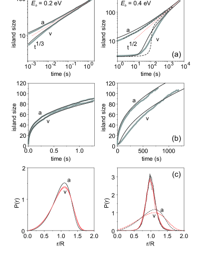
Figure 5: The results of numerical solution of the Becker–Döring equations: time dependencies of the average island sizes in logarithmic (a) and linear (b) scales and the island size distributions (c). The left column presents calculations for the bond energy $E_{b}=0.2$ eV with diffusion-limited kinetics, while the right column shows the results for the bond energy $E_{b}=0.42$ eV with attachment-limited kinetics. The solutions of the Becker–Döring equations are shown in (a) and (b) by black lines, and the results of the kinetic Monte Carlo simulations by gray lines. Symbols “a” and “v” on the plots denote the results for adatom and advacancy islands, respectively. Full lines in the right column show the calculations for the discrete island energies with ‘magic’ sizes, while the broken lines are calculations for the continuous Gibbs-Thomson chemical potential.

Figure 5 presents the results of the numerical solution of the Becker–Döring equations for adatom and advacancy islands. With the aim to quantitatively compare the solutions with the results of kinetic Monte Carlo simulations in the whole time interval, we obtain the average island sizes in the same way as in the simulations, and use the same initial conditions. Namely, the average island sizes are calculated taking into account the islands containing at least 6 atoms, for the reasons discussed in Sec. II.3. The initial random adatom distribution with the coverage 0.1 ML contains not only monomers, but also dimers, trimers, etc., the densities of which quickly decrease with the increasing number of atoms in the cluster. By simple statistical analysis of the initial distribution in kinetic Monte Carlo simulations, we find that at $t=0$, $c_{n}\approx c_{1}\times 10^{(n-1)/2}$. This distribution was used as the initial condition for the Becker–Döring equations. The initial conditions are essential only at the initial stages of coarsening. The results of the calculations do not depend on the initial monomer concentration $c_{1}$, as long as the initial supersaturation $c_{1}(t=0)/c_{\infty\mathrm{eq}}$ is much larger than unity. The time scales of the solutions are adjusted to these of the Monte Carlo simulations.

The case of small bond energies (left column in Fig. 5) is well described by the 2D diffusion limited kinetics with screening (15) and the ratio of the detachment and the attachment coefficients given by the Gibbs–Thomson formula (8). Calculations in the left column of Fig. 5 are made with $\gamma=3.7$. The solutions of the Becker–Döring equations (black lines) are in a good agreement with the results of the kinetic Monte Carlo simulations (gray lines), that are repeated from Fig. 1. The coarsening laws for adatom and advacancy islands almost coincide and quickly reach the Lifshitz–Slyozov $t^{1/3}$ asymptotic. The island size distributions, Fig. 5(c), also almost coincide for adatom and advacancy islands, possess kinetic scaling, and agree well with these obtained in the kinetic Monte Carlo simulations, cf. Fig. 1(d).

For large bond energies (right column in Fig. 5), the calculations are performed with attachment-limited kinetics, Eq. (18), since the kinetic Monte Carlo simulations point to the Wagner’s $t^{1/2}$ asymptotic. We compare the discrete distribution of the island energies that takes into account the ‘magic’ island sizes as described in Sec. III.2 (full black lines) with the continuous one, given by the Gibbs–Thomson formula (broken lines). The relationship between the discrete and the continuous models is established by calculating the energy of a square island and a circular one with the same number of atoms: $E_{b}/k_{\mathrm{B}}T=\sqrt{\pi}\gamma/2$. The calculations are performed for $\gamma=7$. The effect of magic sizes is slightly different for adatom and advacancy islands. For adatom islands, the detachment coefficients $b_{n}$ given by Eq. (14) are exceptionally large for $n=m+1$, where $m$ is a magic number. Thus, a monomer that has attached to a magic island detaches again with a high probability. For advacancy islands, the detachment coefficients $b_{m}$ for magic islands are exceptionally small, so that the detachment of an atom from a vacancy island (this atom becomes an adatom on the higher level) proceeds at a small rate. Both processes make each magic size a trap for further island growth, giving rise to the discrete island size distribution peaked at the magic sizes, shown in Fig. 4. The island size distributions presented in Fig. 5(c) for this case are obtained by averaging over finite ranges of the sizes, in the same way as done in the kinetic Monte Carlo simulations.

The time dependence of the average island sizes obtained for coarsening through the sequence of magic islands (full black lines in right column of Fig. 5) are in good agreement with the results of kinetic Monte Carlo simulations (gray lines). For vacancy islands, the continuous island size distribution with the Gibbs–Thomson formula gives rise to a notably different coarsening behavior (broken lines), with a very fast increase of the island sizes in an intermediate range. The island size distributions obtained in the discrete (with magic sizes) and the continuous models are also notably different, see Fig. 5(c). The distribution obtained in the discrete model is symmetric with respect to the maximum, similar to the one obtained in the Monte Carlo simulations, but notably narrower, cf. Fig. 1(d). It is worth to note that the distribution scaled by the average island size does not change in time and is the same for the adatom and advacancy islands, despite the time evolutions of the average island sizes not coinciding and not following a power law. In other words, the solution of the Becker–Döring equation obeys kinetic scaling in the sense that the island size distribution is a function of $r/R(t)$ that does not depend on time. However, $R(t)$ is not described by a power law. The continuous model gives a much broader and asymmetric island size distribution, shown by broken lines in Fig. 5(c). The broken-bond counting scheme described in Sec. III.2 adequately represents the energies $E_{n}$ of small islands and quantitatively describes the island size distribution at the initial stage of coarsening, see Fig. 4. However, for larger islands it oversimplifies the island energy distribution and gives rise to a more narrow distribution than found in the simulations. A better model for the island energies $E_{n}$ is needed to describe this distribution correctly.

To summarize this section, we show that the Ostwald ripening kinetics can be described as an initial value problem for ordinary differential equations (1)–(8) that can be solved by standard numerical methods. This approach can be applied to various coarsening problems by replacing the Gibbs–Thomson formula (8) with Eqs. (14), (23) that admit any dependence of the island energy $E_{n}$ on the number of atoms $n$ in it. The alternative approach, a numerical implementation of the integro-differential equations (9)–(11),Venzl (1983); Carillo and Goudon (2003) seems much more difficult.

IV Conclusions

Our kinetic Monte Carlo simulations show that the Ostwald ripening of 2D islands qualitatively changes with increasing bond energy (or decreasing temperature). The islands become faceted and the coarsening proceeds through a sequence of magic sizes. The Gibbs-Thomson chemical potential is not applicable and the detachment of monomers from islands is governed by the discrete energies of the islands. The coarsening is diffusion limited at small bond energies and becomes attachment limited at large bond energies. In this latter case, Wagner’s asymptotic law is reached only after a very long transient regime.

We show that the Becker–Döring equations of nucleation kinetics are well suited to study the process of Ostwald ripening. Two- and three-dimensional coarsening processes with diverse limiting mechanisms can be simulated by solving a system of ordinary differential equations. Concentrations of clusters of all sizes, from monomers to ones consisting of millions of atoms, can be traced simultaneously. The calculations are not necessarily based on the Gibbs–Thomson formula but adopt any continuous or singular dependence of the cluster energy on the number of atoms in it. This approach can be applied to a wide range of coarsening problems for two- and three-dimensional islands on a surface.