Statistical Cryptography using a Fisher-Schrödinger Model

Abstract

A principled procedure to infer a hierarchy of statistical distributions possessing ill-conditioned eigenstructures, from incomplete constraints, is presented. The inference process of the pdf’s employs the Fisher information as the measure of uncertainty, and, utilizes a semi-supervised learning paradigm based on a measurement-response model. The principle underlying the learning paradigm involves providing a quantum mechanical connotation to statistical processes. The inferred pdf’s constitute a statistical host that facilitates the encryption/decryption of covert information (code). A systematic strategy to encrypt/decrypt code via unitary projections into the null spaces of the ill-conditioned eigenstructures, is presented. Numerical simulations exemplify the efficacy of the model.

1 . Introduction

This paper accomplishes a two-fold objective. First, a systematic methodology to infer from incomplete constraints, a hierarchy of statistical distributions corresponding to the multiple energy states of a time independent Schrödinger-like equation (TIS-lE), is presented. By definition, the case of incomplete constraints corresponds to scenarios where the number of constraints (physical observables) is less than the dimension of the distribution. The inference procedure employs a semi-supervised learning paradigm, based on a measurement-response model that utilizes the Fisher information (FI) as the measure of uncertainty.

The time independent Schrödinger equation (TISE) is a fundamental equation of physics, that describes the behavior of a particle in the presence of an external potential [1]

$$\underbrace{-\frac{{\hbar^{2}}}{{2m}}\frac{{d^{2}\psi\left(x\right)}}{{dx^{2}}}+V\left(x\right)\psi\left(x\right)}_{H^{QM}\psi\left(x\right)}=E\psi\left(x\right).\$$ (1)

Here, $\psi\left(x\right)$ is the wave function, $E$ is the total energy eigenvalue,$V(x)$ is the external potential, and, $H^{QM}$ is the TISE Hamiltonian. The constants $\hbar$ and $m$ are the Planck constant and the particle mass, respectively. In time independent scenarios, Lagrangians containing the FI as the measure of uncertainty, yield on variational extremization an equation similar to the TISE, i.e. the TIS-lE [2] . The TIS-lE provides a quantum mechanical connotation to a statistical process.

Next, a self-consistent strategy to project covert information into the null spaces of ill-conditioned eigenstructures possessed by the inferred host statistical distributions corresponding to the multiple energy states of the TIS-lE, is described. The strategy of unitary projection of covert information into the null spaces of the ill conditioned eigenstructures of a hierarchy of statistical distributions, has been recently studied for host probability density functions (pdf’s, hereafter) inferred using the maximum entropy (MaxEnt) principle [3].

The selective projection of covert information into a hierarchy of statistical distributions implies that the dimension of the covert information is greater than that of any single host distribution. This selective projection endows the code with multiple layers of security, without altering the host statistical distributions. The present paper accomplishes the task of achieving both symmetric and asymmetric cryptography [4] via a judicious amalgamation of statistical inference using an information theoretic semi-supervised learning paradigm, quantum mechanics, and, the theory of unitary projections.

In summary, the semi-supervised learning paradigm is utilized to infer the statistical hosts possessing ill-conditioned eigenstructures. The code is then projected into the null spaces of these ill-conditioned eigenstructures. Another example of the use of learning theory in cryptosystems, albeit within a different context, is described in [5].

1.1 The TIS-lE

Consider a measured random variable $y=\left({y_{1},...,y_{N}}\right)$, parameterized by $\theta=\left({\theta_{1},...,\theta_{N}}\right)$ (the ”true” value). A fluctuation, i.e. a random variable $x=\left({x_{1},...,x_{N}}\right)$, defined by $x=y-\theta$ is introduced. For translational (or shift) invariant families of distributions, $p\left({y\left|\theta\right.}\right)=p\left({y-\theta}\right)=p\left(x\right)$. The particular form of the FI that is chosen is the trace of the FI matrix for independent and identically distributed (iid, hereafter) data . This is referred to as the Fisher channel capacity (FCC) [2]. The FCC is: $I^{FCC}=\int{dyp\left({\left.y\right|\theta}\right)}\left({\frac{{\partial\ln p\left({\left.y\right|\theta}\right)}}{{\partial\theta}}}\right)^{2}=\int{dxp\left(x\right)}\left({\frac{{\partial\ln p\left(x\right)}}{{\partial x}}}\right)^{2}$ under translational invariance [2,6]. The probability amplitude (wave function) relates to the pdf as $\psi\left(x\right)=\sqrt{p\left(x\right)}$. The FCC acquires the compact form $I^{FCC}=4\sum\limits_{n=1}^{N}{\int{dx_{n}\left({\frac{{\partial\psi\left({x_{n}}\right)}}{{\partial x_{n}}}}\right)}^{2}}=4\int{dx\left({\frac{{\partial\psi\left(x\right)}}{{\partial x}}}\right)}^{2}$. The form of the FCC is essential to the formulation of a variational principle. Within the framework of a measurement-response model, this implies that the observer who initiates the measurements, collects the response in the form of iid data. In many practical scenarios, the response of a system to measurements is not obliged to be iid. The presence of correlations contribute to off-diagonal elements in the FI matrix formed by the observer. These correlations may be mitigated, thereby eliminating the off-diagonal elements of the FI matrix, by performing ICA (or an equivalent procedure) as a pre-processing stage.

Consider a Lagrangian of the form

$$\begin{array}[]{l}L^{FCC}=4\int{dx\left({\frac{{\partial\psi\left(x\right)}}{{\partial x}}}\right)}^{2}+\\ +\underbrace{\int{dx\sum\limits_{i=1}^{M}{\lambda_{i}\Theta_{i}\left(x\right)\psi^{2}\left(x\right)}-\lambda_{o}\int{dx\psi^{2}\left(x\right)}}}_{-J\left[x\right]},\\ \end{array}$$ (2)

$M<N$ (incomplete constraints), where the Lagrange multiplier (LM) $\lambda_{o}$ corresponds to the probability density function (pdf, hereafter) normalization condition $\int{dx\psi^{2}\left(x\right)}=1$. The LM’s $\lambda_{i};i=1,...,M$ correspond to actual (physical) constraints of the form $\int{dx\Theta_{i}\left(x\right)\psi^{2}\left(x\right)}=\left\langle{\Theta_{i}\left(x\right)}\right\rangle=d_{i}$. Here, $\Theta_{i}\left(x\right)$ are operators, and, $d_{i}$ are the constraints (physical observables). This work considers constraints of the geometric moment type: $\Theta_{i}\left(x\right)=x^{i};i=0,...,M$. Here, (2) resembles the usual MaxEnt Lagrangian with the FCC replacing the Shannon entropy. In (2), the FCC is ascribed the role akin to the kinetic energy. The constraint terms manifest the potential energy. Variational extremization of (2) yields the minimum Fisher information (MFI) principle [7]

$$\underbrace{-\frac{{d^{2}\psi\left(x\right)}}{{dx^{2}}}+\frac{1}{4}\sum\limits_{i=1}^{M}{\lambda_{i}\Theta_{i}\left(x\right)}\psi\left(x\right)}_{H^{FI}\psi\left(x\right)}=\frac{{\lambda_{o}}}{4}\psi\left(x\right),\$$ (3)

where $H^{FI}$ is an empirical Hamiltonian operator. Here, (3) is referred to as a TIS-lE. Note that the probability amplitudes are taken as being real quantities. This assumption is tenable since the model is spatially one dimensional in the continuum, and is time independent. Comparing the TIS-lE with the TISE immediately reveals that the constraint terms $V\left(x\right)=\frac{1}{4}\sum\limits_{i=1}^{M}{\lambda_{i}}\Theta_{i}\left(x\right)=\sum\limits_{i=1}^{M}{\tilde{\lambda}_{i}}x^{i}$, constitute an empirical pseudo-potential. The normalization LM and the total energy eigenvalue relate as $\lambda_{o}=4E$. Further, the constants in the TISE relate as ${{\hbar^{2}}\mathord{\left/{\vphantom{{\hbar^{2}}{2m}}}\right.\kern-1.2pt}{2m}}=1$.

Solution of the TISE as an eigenvalue problem yields a number of energy states characterized by distinct values of $E$. These comprise the equilibrium state (zero-energy state) characterized by a Maxwellian distribution, and, higher energy excited states (non-equilibrium states). The wave functions are a superposition of Hermite-Gauss solutions. By virtue of its similarity to the TISE, the TIS-lE “inherits” these energy states within an information theoretic context. This feature permits the projection of covert information into multiple energy states of the TIS-lE, for an empirical pseudo-potential that approximates a TISE physical potential.

Employing the TIS-lE to infer pdf’s from incomplete constraints, requires an accurate evaluation of the LM’s. This is accomplished in this paper through a semi-supervised learning paradigm, that iteratively couples the solution of (3) with the minimization of a Lagrangian that manifests a measurement-response model.

This procedure represents, in certain aspects, an extension of the optimization procedure employed to achieve quantum clustering using the TISE [8]. In the case of quantum clustering, the TISE probability amplitude/wave function is approximated by a non-parametric estimator (Parzen windows), and, the potential $V(x)$ is determined via a steepest descent in Hilbert space. In contrast, the semi-supervised paradigm presented in this paper achieves reconstruction of pdf’s (the inverse problem of statistics) without any a-priori strictures placed on the probability amplitudes of (3). The Fisher-Schrödinger model has been employed within a statistical setting in a number of studies ranging from quantum statistics to fuzzy clustering [9]. Within the context of securing covert information, the above features endow the statistical enryption/decryption strategy with a fundamental physical connotation.

1.2 The Dirac notation

This paper utilizes the Dirac bra-ket notation [10] to describe linear algebraic operations in a compact form. By definition, a ket $\left|\bullet\right\rangle$ denotes a column vector, and, a bra $\left\langle\bullet\right|$ denotes a row vector. The scalar inner product and the projection operators are described by $\left\langle{\bullet}\mathrel{\left|{\vphantom{\bullet\bullet}}\right.\kern-1.2pt}{\bullet}\right\rangle$, and the outer product $\left|\bullet\right\rangle\left\langle\bullet\right|$, respectively. The expectation evaluated at the $\varepsilon^{th}$ energy state is $\left\langle\bullet\right\rangle_{\varepsilon}$.

2 Semi-supervised Learning Paradigm

2.1 Theory

The task of density estimation involves the iterative determination of the LM’s and probability amplitudes of the TIS-lE (3). In the MaxEnt and MFI theories, the observer is external to the system. The present work reconstructs the host pdf’s using a semi-supervised learning paradigm, by incorporating a participatory observer. This is accomplished by positioning the participatory observer in a measurement space characterized by the amplitude $\psi^{\varepsilon}(x)$, performing unbiased measurements [2, 11] on a given physical system (data).

The system space, inhabited by the physical system subject to measurements, is characterized by an amplitude $\phi^{\varepsilon}(\tilde{x})$. Here, $x$ and $\tilde{x}$ are the conjugate basis coordinates of the measurement space and system space, respectively. Herein, the mutually conjugate spaces are taken to be the Cartesian coordinate and the linear momentum. Setting $\tilde{x}=\mu$, the commutation relation is $\left[{x,\mu}\right]=i\hbar$, respectively [1]. The group for the basis change is $G=-i\hbar\frac{d}{{dx}}$. The corresponding Hermitian unitary operator is $U=e^{-ai\hbar\frac{d}{{dx}}}$, where $a$ is the group parameter of infinitesimal transformations. Within the present scenario, $U\psi^{\varepsilon}\left[x\right]=\varphi^{\varepsilon}\left[{\mu}\right]$. On the basis of the above discussions, it is easily proven that $I_{\varepsilon}^{FCC}\left[x\right]=4\int{dx\left({\frac{{d\psi\left(x\right)}}{{dx}}}\right)}^{2}=\frac{4}{{\hbar^{2}}}\left\langle{\mu^{2}}\right\rangle_{\varepsilon}=4\left\langle{\frac{{\mu^{2}}}{{2m}}}\right\rangle_{\varepsilon}=I_{\varepsilon}^{FCC}\left[\mu\right];{\raise 3.01385pt\hbox{${\hbar^{2}}$}\!\mathord{\left/{\vphantom{{\hbar^{2}}{2m}}}\right.\kern-1.2pt}\!\lower 3.01385pt\hbox{${2m}$}}=1$. In the non-relativistic limit, the kinetic energy of a particle is $T=\frac{{\mu^{2}}}{{2m}}$ [1]. For TIS-lE polynomial pseudo-potentials of the form $V\left(x\right)=\sum\limits_{i=1}^{M}{\lambda_{i}^{\varepsilon}x^{i}}$, the quantum mechanical virial theorem [9, 12, 13] yields

$$I_{\varepsilon}^{FCC}\ =2\left\langle{x\frac{{dV\left(x\right)}}{{dx}}}\right\rangle_{\varepsilon}=2\sum\limits_{i=1}^{M}{i\lambda_{i}^{\varepsilon}d_{i}^{\varepsilon}}\$$ (4)

The unitary relation between the amplitudes in conjugate spaces results in the potential energy term in (2), $J_{\varepsilon}\left[x\right]$, being manifested as an empirical representation of the FCC. Specifically, $I_{\varepsilon}^{FCC}\left[x\right]=J_{\varepsilon}\left[x\right]$. Each measurement (or set of measurements) initiated by the observer at a specific juncture, perturbs the amplitude of the system space as $\delta\varphi^{\varepsilon}\left({\mu}\right)$. For mutually conjugate spaces related by a unitary transform, this results in a perturbation $\delta\psi^{\varepsilon}\left(x\right)=\delta\varphi^{\varepsilon}\left({\mu}\right)$ of the measurement space. It is at this juncture that the observer constructs the FCC for iid data. Consequently, $\delta I_{\varepsilon}^{FCC}\left[x\right]=\delta J_{\varepsilon}\left[x\right]$ [2]. Such models are known as measurement-response models [14].

Incorporation of a participatory observer results in a zero-sum game [15] of information acquisition played between the observer and the system under observation. The observer seeks to maximize her/his information about the system. Simultaneously, the system space is inhabited by a demon, remniscent to the Maxwell demon, who seeks to minimize this information transfer. This zero-sum game between the observer and the demon is hereafter referred to as the Fisher game.

Game theoretic studies in MaxEnt and MFI follow the traditional pattern of having the arbiter, who assigns strategies to the players, residing external to the system. In this paper, the probe measurements initiated by the observer constitute the arbiter, and, the probability amplitudes manifest the strategies. A future publication treats the game theoretic aspects of the semi-supervised learning paradigm, within the ambit of the bounded rationality theory [16].

The incomplete constraints ${d_{i}^{\varepsilon}},i=1,...,M$ are evaluated as the moments of the Cartesian coordinates at each energy state $\varepsilon$, by solving the TISE (1) as an eigenvalue problem on a lattice, for an a-priori specified physical potential. The incomplete constraints represent the only manifestation of the target values of the amplitudes/pdf’s, made available to the designer at the commencement of the inference procedure.

The host pdf inference is solved by an iterative optimization process In this paper, the host pdf is independently inferred for each energy level $\varepsilon$. The optimization process couples the solution of the TIS-lE (3), with the steepest descent minimization of an empirical quantity known as the residue. The residue represents the discrepancy between the value of $J_{\varepsilon}\left[x\right]$ in (2) evaluated at an intermediate iteration level $l$ for a specific energy state, and, the value of the exact (target) FCC expressed at the same iteration level $l$.

In (4), the LM’s $\lambda_{i}^{\varepsilon}$ are target values of the optimization process, which are unknown at the commencement of the inference procedure. Here, (4) is made consistent with the iteration process by specifying the relation between the target values of the LM’s, and, the LM’s at some intermediate iteration level $l$ as

$$\begin{array}[]{l}2\sum\limits_{i=1}^{M}{i\lambda_{i}^{\varepsilon}}\cong\sum\limits_{i=1}^{M}{\lambda_{i,l}^{\varepsilon}\left\langle{{\psi_{l}^{\varepsilon}}}\mathrel{\left|{\vphantom{{\psi_{l}^{\varepsilon}}{\psi_{l}^{\varepsilon}}}}\right.\kern-1.2pt}{{\psi_{l}^{\varepsilon}}}\right\rangle}_{\varepsilon}\end{array}$$ (5)

Here, (5) is critical to the optimization process since it infuses a representation of the target response state into the iterative procedure. The final values of the expectation of the amplitudes satisfy $\left\langle{{\psi_{l=final}^{\varepsilon}}}\mathrel{\left|{\vphantom{{\psi_{l=final}^{\varepsilon}}{\psi_{l=final}^{\varepsilon}}}}\right.\kern-1.2pt}{{\psi_{l=final}^{\varepsilon}}}\right\rangle_{\varepsilon}=1$. Note that the expectation ${\left\langle{{\psi_{l}^{\varepsilon}}}\mathrel{\left|{\vphantom{{\psi_{l}^{\varepsilon}}{\psi_{l}^{\varepsilon}}}}\right.\kern-1.2pt}{{\psi_{l}^{\varepsilon}}}\right\rangle}_{\varepsilon}$ is not assumed to be unity. Combining (4) and (5) allows the target value of the FCC to be manifested at some intermediate iteration level $l$. At the $\ l^{th}\$ iteration level, the term $J_{\varepsilon}[x]$ in (2) is

$$\begin{array}[]{l}J\left({\lambda_{i,l}^{\varepsilon}}\right)=\lambda_{o,l}^{\varepsilon}\left\langle{{\psi_{l}^{\varepsilon}}}\mathrel{\left|{\vphantom{{\psi_{l}^{\varepsilon}}{\psi_{l}^{\varepsilon}}}}\right.\kern-1.2pt}{{\psi_{l}^{\varepsilon}}}\right\rangle_{\varepsilon}-\sum\limits_{i=1}^{M}{\lambda_{i,l}^{\varepsilon}\left\langle{\psi_{l}^{\varepsilon}}\right|\Theta\left(x\right)\left|{\psi_{l}^{\varepsilon}}\right\rangle}_{\varepsilon}\\ \end{array}$$ (6)

The residue at the $l^{th}$ iteration level, re-scaled with respect to $\left\langle{{\psi_{l}^{\varepsilon}}}\mathrel{\left|{\vphantom{{\psi_{l}^{\varepsilon}}{\psi_{l}^{\varepsilon}}}}\right.\kern-1.2pt}{{\psi_{l}^{\varepsilon}}}\right\rangle_{\varepsilon}$, is

$$\begin{array}[]{l}\frac{{R_{\varepsilon}\left({\lambda_{i,l}^{\varepsilon}}\right)}}{{\left\langle{{\psi_{l}^{\varepsilon}}}\mathrel{\left|{\vphantom{{\psi_{l}^{\varepsilon}}{\psi_{l}^{\varepsilon}}}}\right.\kern-1.2pt}{{\psi_{l}^{\varepsilon}}}\right\rangle_{\varepsilon}}}=\tilde{R}_{\varepsilon}\left({\lambda_{i,l}^{\varepsilon}}\right)\\ \cong-\lambda_{o,l}^{\varepsilon}+\sum\limits_{i=1}^{M}{\lambda_{i,l}^{\varepsilon}\left\{{\frac{{\left\langle{\psi_{l}^{\varepsilon}}\right|\Theta\left(x\right)\left|{\psi_{l}^{\varepsilon}}\right\rangle_{\varepsilon}}}{{\left\langle{{\psi_{l}^{\varepsilon}}}\mathrel{\left|{\vphantom{{\psi_{l}^{\varepsilon}}{\psi_{l}^{\varepsilon}}}}\right.\kern-1.2pt}{{\psi_{l}^{\varepsilon}}}\right\rangle}_{\varepsilon}}+d_{i}^{\varepsilon}}\right\}}\\ \end{array}$$ (7)

Here, (7) is $\tilde{R}_{\varepsilon}\left({\lambda_{i,l}^{\varepsilon}}\right)\cong\tilde{I}_{\varepsilon}^{FCC}\left({\lambda_{i,l}^{\varepsilon},d_{i}^{\varepsilon}}\right)-\Im_{\varepsilon}\left({\lambda_{o,l}^{\varepsilon},\lambda_{i,l}^{\varepsilon}}\right);i=1,...,M$, where the re-scaled target FCC and the potential energy are $\tilde{I}_{\varepsilon}^{FCC}\left({\lambda_{i,l}^{\varepsilon},d_{i}^{\varepsilon}}\right)\$, and, $\ \Im_{\varepsilon}\left({\lambda_{o,l}^{\varepsilon},\lambda_{i,l}^{\varepsilon}}\right)$, respectively. A steepest descent procedure $\frac{{\partial\tilde{R}_{\varepsilon}\left({\lambda_{i,l}^{\varepsilon}}\right)}}{{\partial\lambda_{i,l}^{\varepsilon}}}\to 0$ along the gradient of the LM’s yields “optimal” values of the LM’s

$$\frac{{\partial\left[{\tilde{I}_{\varepsilon}^{FCC}\left({\lambda_{i,l}^{\varepsilon},d_{i}^{\varepsilon}}\right)-\Im_{\varepsilon}\left({\lambda_{o,l}^{\varepsilon},\lambda_{i,l}^{\varepsilon}}\right)}\right]}}{{\partial\lambda_{i,l}^{\varepsilon}}}\to 0;i=1,...,M\\$$ (8)

The optimization procedure is carried out till the target values are achieved. The steepest descent procedure requires the analytical values of $\frac{{\partial\tilde{R}_{\varepsilon}\left({\lambda_{i,l}^{\varepsilon}}\right)}}{{\partial\lambda_{i,l}^{\varepsilon}}}$, and thus, $\frac{{\partial\lambda_{o,l}^{\varepsilon}}}{{\partial\lambda_{i,l}^{\varepsilon}}};i=1,...,M$. Left multiplying (3) for the energy state $\varepsilon$ and iteration level $l$ by ${\psi_{l}^{\varepsilon}}$ and integrating, yields $\frac{{\partial\lambda_{o,l}^{\varepsilon}}}{{\partial\lambda_{i,l}^{\varepsilon}}}=\frac{{d_{i,l}^{\varepsilon}}}{{\left\langle{{\psi_{l}^{\varepsilon}}}\mathrel{\left|{\vphantom{{\psi_{l}^{\varepsilon}}{\psi_{l}^{\varepsilon}}}}\right.\kern-1.2pt}{{\psi_{l}^{\varepsilon}}}\right\rangle_{\varepsilon}}};i=1,...,M$. The theory of the semi-supervised learning paradigm based on the Fisher game is summarized by the pseudo-code in Algorithm 1.

2.2 Physical interpretations

The Fisher game constitutes a self-consistent information theoretic optimization procedure, with a quantum mechanical connotation. The above theory contains three interesting observations. First, the commencement of each iteration loop corresponds to the juncture at which the observer initiates measurements. Next, as the iterative process advances, the FCC approaches a minimum. This corresponds to an increase in the uncertainty at the location of the observer.

Finally, at the termination of the $l^{th}$ iteration loop, the condition (8) that yields the ”optimal” LM’s is the statement of a contract between the demon and the observer, whereby, the demon makes the last move in the iterative Fisher game. This implies that the participatory observer acquires a state of maximum uncertainty (minimum Fisher information). Such a contract is the underlying basis for determining the ”optimal” LM’s, corresponding to amplitudes that decrease the FCC at the termination of each iteration level.

Scenarios of such type cannot be modeled within the framework of traditional game theory [17], thus, justifying the use of the bounded rationality theory to study the game theoretic aspects of the Fisher game. A future publication studies the information landscape and its relation to the Fisher game.

Algorithm 1 Inverse Problem of Statistics

  PROCEDURE FOR EACH ENERGY STATE $\varepsilon$

  INITIALIZATION 1.Solve TISE (1) for known physical potential $V(x)$ as an eigenvalue problem in the event space $\left[{a,b}\right]$. Obtain incomplete constraints $d_{i}^{\varepsilon};i=1,...,M$. 2. Solve TIS-lE (3) for arbitrary Lagrange multipliers $\lambda_{i,arbitrary}^{\varepsilon};i=1,...,M$. Obtain amplitudes $\psi_{i,l=1}^{\varepsilon}$. 3. Input tolerance parameter $\delta_{i};i=1,...,M$

  ALGORITHM FOR $l^{th}\geq 1$ ITERATION LOOP 1. Obtain $\psi_{l}^{\varepsilon}$ by solving the TIS-lE (3) as an eigenvalue problem, using the optimized LM’s $\lambda_{i,l-1}^{\varepsilon}$ obtained from the $(l-1)^{th}$ iteration loop. 2. Minimize the re-scaled residue $\tilde{R}_{\varepsilon}\left({\lambda_{i,l}^{\varepsilon}}\right)$ (7), to obtain optimized LM’s that correspond to $\psi_{l}^{\varepsilon}$ $\lambda_{i,l}^{\varepsilon}\leftarrow\frac{{\partial\left[{\tilde{I}_{\varepsilon}^{FCC}\left({\lambda_{i,l}^{\varepsilon},d_{i}^{\varepsilon}}\right)-\Im_{\varepsilon}\left({\lambda_{o,l}^{\varepsilon},\lambda_{i,l}^{\varepsilon}}\right)}\right]}}{{\partial\lambda_{i,l}^{\varepsilon}}}$ 3. Solve TIS-lE (3) as an eigenvalue problem with LM’s $\lambda_{i,l}^{\varepsilon}$. Obtain moments $d_{i,l}^{\varepsilon};i=1,...,M$.

  IF $\left|{d_{i}^{\varepsilon}-d_{i,l}^{\varepsilon}}\right|>\delta_{i};i=1,...,M$ $l=l+1$

  RETURN

  ELSE IF $\left|{d_{i}^{\varepsilon}-d_{i,l}^{\varepsilon}}\right|\leq\delta_{i};i=1,...,M$

  END IF

2.3 Numerical results

The asymmetric harmonic oscillator (AHO) potential $V\left(x\right)=x+\frac{{x^{2}}}{2}$ is chosen as TISE physical potential. The TISE with the AHO potential is solved as an eigenvalue problem for 201 data points within the event space $\left[{a=-1,b=1}\right]$ for different energy states. Boundary conditions on the amplitudes, $\psi^{\varepsilon}\left(a\right)=\psi^{\varepsilon}\left(b\right)=0$, are enforced. An empirical pseudo-potential of the form $V_{\varepsilon}\left(x\right)=\tilde{\lambda}_{1}^{\varepsilon}x+\tilde{\lambda}_{2}^{\varepsilon}$, that approximates the TISE AHO physical potential is specified. Here, $\tilde{\lambda}_{i}^{\varepsilon}=\frac{{\lambda_{i}^{\varepsilon}}}{4}$. In this case, $M=2,N=201$.

The values of the incomplete constraints are $d_{1}^{\varepsilon=0,1}=({\rm-0}{\rm.0344},{\rm 0}{\rm.0097,}),and,d_{2}^{\varepsilon=0,1}=({\rm 0}{\rm.1302},{\rm 0}{\rm.2809})$. The final values of the LM’s are $\tilde{\lambda}_{1}^{\varepsilon=0,1}=({\rm 1}{\rm.0892},{\rm 1}{\rm.1121})$, and, $\tilde{\lambda}_{2}^{\varepsilon=0,1}=({\rm 0}{\rm.6635},{\rm 0}{\rm.7175})\$, respectively. The inferred total energy eigenvalues are $\ E_{\inf}^{\varepsilon=0,1}=({\rm 2}{\rm.5333},{\rm 10}{\rm.0769})\$. The corresponding TISE total energy eigenvalues are $\ E_{exact}^{\varepsilon=0,1}=(2.5152,{\rm 10}{\rm.0147})\$. Fig. 1 depicts the inferred pdf’s overlaid upon the TISE solution. Here, the Maxwellian distribution corresponds to $\varepsilon=0$, and, double peaked pdf corresponds to the first excited state $\varepsilon=1$. Note that the inferred pdf’s almost exactly coincide with the TISE solutions.

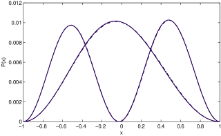
Figure 1: Inferred TIS-lE pdf (dash-dots) and exact TISE pdf (solid lines)

3 Projection Strategy

Consider $\ M\$ constraints $\ d_{1}^{\varepsilon},...,d_{M}^{\varepsilon}\$. In a discrete setting, these are expectation values of a random variable $\ x_{i,n};n=1,...,N\$:

$$\ d_{i}^{\varepsilon}=\sum\limits_{n=1}^{N}{p_{n}^{\varepsilon}x_{i,n}};i=1,...,M.\$$ (9)

The pdf $\left|p^{\varepsilon}\right\rangle\in\Re^{N}$ is a ket, where $\left|n\right\rangle;n=1,...,N$ is the standard basis in $\Re^{N}$, is expressed as $\left|p^{\varepsilon}\right\rangle=\sum\limits_{n=1}^{N}{\left|n\right\rangle\left\langle{n}\mathrel{\left|{\vphantom{np}}\right.\kern-1.2pt}{p^{\varepsilon}}\right\rangle}=\sum\limits_{n=1}^{N}{p_{n}^{\varepsilon}\left|n\right\rangle}$. The ket of observable’s is expressed as $\left|d^{\varepsilon}\right\rangle\in\Re^{M+1}$ with components $d_{1}^{\varepsilon},...,d_{M}^{\varepsilon},1$, and, an operator $A:\Re^{N}\to\Re^{M+1}$ given by $A=\sum\limits_{n=1}^{N}{\left|{x_{n}}\right\rangle\left\langle n\right|}\$. Defining vectors $\left|{x_{n}}\right\rangle\in\Re^{M+1};n=1,...,N$ as the expansion $\left|{x_{n}}\right\rangle=\sum\limits_{i=1}^{M+1}{\left|i\right\rangle}\left\langle{i}\mathrel{\left|{\vphantom{i{x_{n}}}}\right.\kern-1.2pt}{{x_{n}}}\right\rangle=\sum\limits_{i=1}^{M+1}{x_{i,n}}\left|i\right\rangle$, where $\ i\$ is a basis vector in $\Re^{M+1}$, (9) acquires the compact form

$$\left|{d^{\varepsilon}}\right\rangle=A\left|{p^{\varepsilon}}\right\rangle;A:\Re^{N}\to\Re^{M+1}.\$$ (10)

The physical significance of the constraint operator $A$ in (10) is as follows. Inference of the pdf and the TIS-lE pseudo-potential in (3) from physical observables is achieved by specifying $V\left(x\right)=\sum\limits_{i=1}^{M}{\lambda_{i}}x^{i}$. In a discrete setting, $x_{n}^{i}\to x_{i,n};i=1,...,M;n=1,...,N$. The $x_{i,n}$ constitute the elements of the $M$ rows and $N$ columns of the operator $A$, and represent the spatial elements of the TIS-lE pseudo-potential in matrix form. The unity element in $\left|d^{\varepsilon}\right\rangle\in\Re^{M+1}$ enforces the normalization constraint of the probability density $\left|{p^{\varepsilon}}\right\rangle$.

The operator $A$ is independent of the host pdf, and thus, the energy state. This may be mitigated by defining

$$\tilde{A}^{\varepsilon}=A+k^{\varepsilon}\left|{d^{\varepsilon}}\right\rangle\left\langle I\right|\$$ (11)

Here, $\left\langle I\right|$ is a $1\times N$ bra, and, $k^{\varepsilon}\neq-1$ is a constant parameter introduced to adjust the condition number of $\tilde{A}^{\varepsilon}$, and hence its sensitivity to perturbations. In (11), dependence upon the host pdf is ”injected” into the operator $\tilde{A}^{\varepsilon}$ by the incorporation of $\left|{d^{\varepsilon}}\right\rangle$. Specifically, each element of the ket $\left|{d^{\varepsilon}}\right\rangle$ is defined by $\sum\limits_{n=1}^{N}{p_{n}^{\varepsilon}}x_{n}^{i};i=1,...,M$.

Thus, (10) becomes $\tilde{A}^{\varepsilon}\left|{p^{\varepsilon}}\right\rangle=\left|{d^{\varepsilon}}\right\rangle+\left\langle{k^{\varepsilon}\left|{d^{\varepsilon}}\right\rangle\left\langle I\right|}\right\rangle_{\varepsilon}$. Expanding $\left\langle{k\left|{d^{\varepsilon}}\right\rangle\left\langle I\right|}\right\rangle_{\varepsilon}=k\left|{d^{\varepsilon}}\right\rangle\left\langle I\right|\left.{p^{\varepsilon}}\right\rangle$, and evoking the pdf normalization, $\left\langle I\right|\left.{p^{\varepsilon}}\right\rangle=1$, yields

$$\left|{\tilde{d}^{\varepsilon}}\right\rangle=\left({k^{\varepsilon}+1}\right)\left|{d^{\varepsilon}}\right\rangle=\tilde{A}^{\varepsilon}\left|{p^{\varepsilon}}\right\rangle;\tilde{A}^{\varepsilon}:\Re^{N}\to\Re^{M+1}.\$$ (12)

The operator $\tilde{A}^{\varepsilon}\$is ill-conditioned and rectangular. Thus, (12) becomes:

$$\left|{p^{\varepsilon}}\right\rangle=\left({\tilde{A}^{\varepsilon}}\right)^{-1}\left|{\tilde{d}^{\varepsilon}}\right\rangle+\left|{p^{\varepsilon^{\prime}}}\right\rangle,\$$ (13)

where, ${\left({\tilde{A}^{\varepsilon}}\right)^{-1}}$ is the pseudo-inverse [18] of $\tilde{A}^{\varepsilon}\$, and lies in $range\left({\tilde{A}^{\varepsilon}}\right)$. All necessary data dependent information resides in $\left({\tilde{A}^{\varepsilon}}\right)^{-1}\left|{\tilde{d}^{\varepsilon}}\right\rangle$.

The null space term in (13) is of particular importance since the code is embedded into it via unitary projections. Here, $\left|{p^{\varepsilon^{\prime}}}\right\rangle\in null\left({\tilde{A}^{\varepsilon}}\right)$ is explicitly data independent. However, it is critically dependent on the solution methodology employed to solve (13). The operator $G^{\varepsilon}=\tilde{A}^{\varepsilon{\dagger}}\tilde{A}^{\varepsilon}$ is introduced. Here, $\tilde{A}^{\varepsilon{\dagger}}$ is the conjugate transpose of $\tilde{A}^{\varepsilon}$. Projection of the covert information into $null\left({G^{\varepsilon}}\right)$ instead of $null\left({\tilde{A}^{\varepsilon}}\right)$, leads to increased instability of the eigenstructure, which is exploited to increase the security of the covert information [3, 9].

Given the operator $\tilde{A}^{\varepsilon}$ and the probability vector $\left|p^{\varepsilon}\right\rangle$, whose inference is described in Section 2, the normalized eigenvectors corresponding to the eigenvalues in the null space of $G^{\varepsilon}$ having value zero (zero eigenvalues) are defined as $\left|{\eta_{n}^{\varepsilon}}\right\rangle;n=1,...,N-(M+1)$. Here, $\left|{\eta_{n}^{\varepsilon}}\right\rangle$, defined as the basis of $null\left({G^{\varepsilon}}\right)$, are evaluated using SVD [18]. To introduce cryptographic keys (cryptographic primitives), an operator $\tilde{G}^{\varepsilon}$ is formed by perturbing select elements of $\ G^{\varepsilon}\$ by $\delta G_{i,j}^{\varepsilon}$. Here, $\delta G_{i,j}^{\varepsilon}$ is a perturbation to the element inhabiting the $i^{th}$ row and $j^{th}$ column of the operator $G^{\varepsilon}$. In symmetric cryptography, only a single element of $G^{\varepsilon}\$ is perturbed. The security of the code may be ensured by adopting an asymmetric cryptographic strategy. Here, more than one element of $G^{\varepsilon}$ is perturbed.

The extreme sensitivity to perturbations of $G^{\varepsilon}\$ causes the eigenstructure of ${\tilde{G}^{\varepsilon}=\ G^{\varepsilon}+\delta G_{i,j}^{\varepsilon}}\$ to substantially differ from that of ${G^{\varepsilon}}$, even for infinitesimal perturbations. The values of $\left|{\tilde{\eta}_{n}^{\varepsilon}}\right\rangle;n=1,...,N-(M+1)$, the basis of $null(\tilde{G}^{\varepsilon})$, are evaluated using SVD. The unitary operators of decryption $U_{dec}^{\varepsilon}\$ (without perturbations) and $\tilde{U}_{dec}^{\varepsilon}\$ (with perturbations), $U_{dec}^{\varepsilon},\tilde{U}_{dec}^{\varepsilon}:\Re^{N}\to\Re^{N-(M+1)}$, and, the corresponding encryption operators $U_{enc}^{\varepsilon},\tilde{U}_{enc}^{\varepsilon}\ :\Re^{N-(M+1)}\to\Re^{N}$ for the energy state $\varepsilon$ are

$$\begin{array}[]{l}U_{dec}^{\varepsilon}=\sum\limits_{n=1}^{N-M-1}{\left|n\right\rangle\left\langle{\eta_{n}^{\varepsilon}}\right|};\\ \tilde{U}_{dec}^{\varepsilon}=\sum\limits_{n=1}^{N-M-1}{\left|n\right\rangle\left\langle{\tilde{\eta}_{n}^{\varepsilon}}\right|},\\ and,\\ U_{enc}^{\varepsilon}=U_{dec}^{\varepsilon{\dagger}}=\sum\limits_{n=1}^{N-M-1}{\left|{\eta_{n}^{\varepsilon}}\right\rangle\left\langle n\right|};\\ \tilde{U}_{enc}^{\varepsilon}=\tilde{U}_{dec}^{\varepsilon{\dagger}}=\sum\limits_{n=1}^{N-M-1}{\left|{\tilde{\eta}_{n}^{\varepsilon}}\right\rangle\left\langle n\right|},\\ \end{array}$$ (14)

respectively.

3.1 Encryption

Given a code $\left|q^{\varepsilon}\right\rangle\in\Re^{N-(M+1)}$ to be encrypted in the energy state $\varepsilon$ , the $N-\left({M+1}\right)\$ components are given by $\left\langle{n}\mathrel{\left|{\vphantom{n{q^{\varepsilon}}}}\right.\kern-1.2pt}{{q^{\varepsilon}}}\right\rangle=q_{n}^{\varepsilon};n=1,...,N-\left({M+1}\right)$. The pdf of the embedded code is:

$$\left|{p_{c}^{\varepsilon}}\right\rangle=\tilde{U}_{enc}^{\varepsilon}\left|{q^{\varepsilon}}\right\rangle=\sum\limits_{n=1}^{N-M-1}{\left|{\tilde{\eta}_{n}^{\varepsilon}}\right\rangle\left\langle{n}\mathrel{\left|{\vphantom{n{q^{\varepsilon}}}}\right.\kern-1.2pt}{{q^{\varepsilon}}}\right\rangle}.$$ (15)

The total pdf comprising the host pdf and the pdf of the code is

$$\left|{\tilde{p}^{\varepsilon}}\right\rangle=\left|{p^{\varepsilon}}\right\rangle+\left|{p_{c}^{\varepsilon}}\right\rangle.\$$ (16)

Note that since $\left|{p_{c}^{\varepsilon}}\right\rangle\in null\left({\tilde{A}^{\varepsilon}}\right)\$, $\ \tilde{A}^{\varepsilon}\left|{p_{c}^{\varepsilon}}\right\rangle=0\$.

3.2 Transmission

Information may be transferred from the encrypter to the decrypter in two separate manners , via a public channel. The first mode is to transmit the constraint operators $\tilde{A}^{\varepsilon}$ and the total pdf’s $\left|{\tilde{p}^{\varepsilon}}\right\rangle$. An alternate mode is to transmit the LM’s obtained on solving the Fisher game(Section 2), and, the total pdf’s $\left|{\tilde{p}^{\varepsilon}}\right\rangle$. Owing to the large dimensions of the constraint operators $\tilde{A}^{\varepsilon}$, the latter transmission strategy is more attractive.

The values of parameters $k^{\varepsilon}$ for each energy state, and, the cryptography key/keys are transmitted through a secure/covert channel. The cryptographic primitives are labeled in order to identify the elements of the operator $\ G^{\varepsilon}$ that are perturbed. In the case of asymmetric cryptography, some of the keys may be declared public, while keeping the remainder private [4]. Asymmetric cryptography provides greatly enhanced security to the covert information, and, provides protection against attacks, such as plaintext attacks [3, 4, 9].

3.3 Decryption

The decrypter and encrypter have an a-priori ”agreement” concerning the nature of TIS-lE pseudo-potential, and, the number of energy states. The legitimate receiver recovers the key/keys $\delta G_{i,j}^{\varepsilon}$ and the parameter $k^{\varepsilon}$ from the covert channel. The operators $\tilde{A}^{\varepsilon}\$, $\ G^{\varepsilon}\$, and, $\tilde{G}^{\varepsilon}\$ are constructed. The host pdf may be recovered in two distinct manners, depending upon the transmission strategy employed. Note that both methods to reconstruct the host pdf require the total pdf ${\tilde{p}^{\varepsilon}}$ to be provided by the encrypter. First, the scaled incomplete constraints, defined in (12), are obtained by solving $\ \left\langle i\right|\tilde{A}^{\varepsilon}\left|{\tilde{p}^{\varepsilon}}\right\rangle\ =\ \left|{\tilde{d}^{\varepsilon}}\right\rangle\$. Here, $\ i\$ is a basis vector in $\Re^{M+1}\$. This procedure is possible because $\left|{p_{c}^{\varepsilon}}\right\rangle\in null\left({\tilde{A}^{\varepsilon}}\right)$. Thus, $\ \tilde{A}^{\varepsilon}\left|{p_{c}^{\varepsilon}}\right\rangle=0\$. The host pdf are then computed for each energy state by solving the Fisher game, using the re-scaled set of incomplete constraints. Alternatively, the host pdf may be obtained by solving the TIS-lE (3) as an eigenvalue problem, given the values of the LM’s $\lambda_{i}^{\varepsilon}\ ;i=1,...,M$, and, the event space (Section 2). Both methods allow the reconstructed host pdf’s to be obtained with a high degree of precision. The code pdf is recovered using

$$\left|{p_{rc}^{\varepsilon}}\right\rangle=\left|{\tilde{p^{\varepsilon}}}\right\rangle-\left|{p^{\varepsilon}}\right\rangle.\$$ (17)

The encrypted code is recovered by the operation

$$\left|q_{r}^{\varepsilon}\right\rangle=\tilde{U}_{dec}^{\varepsilon}\left|{p_{rc}^{\varepsilon}}\right\rangle=\sum\limits_{n=1}^{N-M-1}{\left|n\right\rangle\left\langle{{\tilde{\eta}_{n}^{\varepsilon}}}\mathrel{\left|{\vphantom{{\tilde{\eta}_{n}}{p_{rc}^{\varepsilon}}}}\right.\kern-1.2pt}{{p_{rc}^{\varepsilon}}}\right\rangle}\$$ (18)

The thresholds for the cryptographic keys is accomplished by the designer, who performs a simultaneous encryption/decryption without effecting perturbations to the operator $G^{\varepsilon}$. The host pdf’s are inferred from the Fisher game. The code $\left|{q^{\varepsilon}}\right\rangle$ having dimension $N-(M+1)$ is formed. The designer implements (15)-(18) for each energy state $\varepsilon$. The threshold for the cryptographic key/keys is $\delta^{\varepsilon}=\left\|{\left|{q^{\varepsilon}}\right\rangle-\left|{q_{r}^{\varepsilon}}\right\rangle}\right\|$. Hardware independence is demonstrated by performing the encryption on an IBM RS-6000 workstation cluster, and, decryption on an IBM Thinkpad running MATLAB v 7.01. The encryption/decryption strategy is critically dependent upon the exact compatibility of the routines to calculate the basis $\left|{\tilde{\eta}_{n}^{\varepsilon}}\right\rangle$ and the eigenvalue solvers, available to the encrypter and decrypter.

4 Numerical Examples

The encryption/decryption strategy is tested using the energy state dependent model vis-á-vis an energy state independent model [9], for the case of asymmetric cryptography. These are characterized by the constraint operators $\tilde{A}^{\varepsilon}$ (described in (11) and (12)) for $k^{\varepsilon=0,1}=-0.1$, and, $A$ (described in (10)), respectively. The energy state independent model corresponds to the ground state Maxwellian distribution.

A random number generator generates code in $\left[{0,1}\right]$. Two identical kets of the code having dimension $N-(M+1)=198$ are created for projection into the null spaces of the energy state dependent operators $\tilde{G}^{\varepsilon=0,1}$, respectively. This ”emulates” the selective projection of a code comprising of a single ket of dimension $396$, into the two energy state of $null(\tilde{G}^{\varepsilon}$. For the energy state independent operator $null(\tilde{G})$, only a single ket is projected. The cryptographic primitives are $\delta G_{1,3}=\delta\tilde{G}_{1,3}^{\varepsilon=0,1}=3.0e-013$ and $\delta G_{2,7}=\delta\tilde{G}_{2,7}^{\varepsilon=0,1}=7.0e-013$, respectively. All numerical examples in have a threshold for perturbations $\delta^{\varepsilon}\sim 2.0e-014$. The condition numbers, $cond\left(\bullet\right)$ of the constraint operators $A$ and $\tilde{A}^{\varepsilon}$ provides a measure of the sensitivity to perturbations of the operators $G=A^{\dagger}A$ and $G^{\varepsilon}$.

Values of $cond(A)$, $cond(\tilde{A}^{\varepsilon=0})$, and, $cond(\tilde{A}^{\varepsilon=1})$ are ${\rm 3}{\rm.73048}$, $3.{\rm 41742}$, and, ${\rm 3}{\rm.37888}\$, respectively. Going by conventional logic, the energy state independent model should afford greater security to the covert information, owing to the greater value of $cond(A)$, vis-á-vis $cond(\tilde{A}^{\varepsilon=0,1})$. Numerical simulations reveal a dichotomy in this regard.

A more relevant metric of the extreme sensitivity of $null\left({G^{\varepsilon}}\right)$ to perturbations, induced by the cryptographic keys $\delta G_{i,j}^{\varepsilon}$, is the distortion of the code pdf $\left|{p_{c,unpert}^{\varepsilon}}\right\rangle$. Here, $\left|{p_{c,unpert}^{\varepsilon}}\right\rangle$ is evaluated from (15), using $\eta_{n}^{\varepsilon}$ (the unperturbed basis of $null\left({G^{\varepsilon}}\right)$). The distorted code pdf is $\left|{\tilde{p}_{c}^{\varepsilon}}\right\rangle$, which is calculated from (15) using $\tilde{\eta}_{n}^{\varepsilon}$ (the perturbed basis of $null\left({\tilde{G}^{\varepsilon}}\right)$), as described in Section 3.1.

For the energy state dependent model, the RMS error of encryptionis defined as: $RMS_{enc}^{\varepsilon}=\frac{{\left\|{err_{enc}^{\varepsilon}}\right\|}}{{\sqrt{length\left({err_{enc}^{\varepsilon}}\right)}}}$. Here, $\left\|{\left|{err_{enc}^{\varepsilon}}\right\rangle}\right\|\ =\left\|{\left({\left|{p_{c}^{\varepsilon}}\right\rangle-\left|{p_{c,unpert}^{\varepsilon}}\right\rangle}\right)}\right\|\$, and, $length\left({\left|{err_{enc}^{\varepsilon}}\right\rangle}\right)$ is the dimension of $\left({\left|{p_{c}^{\varepsilon}}\right\rangle-\left|{p_{c,unpert}^{\varepsilon}}\right\rangle}\right)$.

A further quantitative metric of the degree of security of the encrypted code is the RMS error of reconstruction between the embedded code and the code reconstructed without the keys. For the energy state dependent model, this is: $RMS_{recon}^{\varepsilon}={\raise 3.01385pt\hbox{${\left\|{\left|{err_{recon}^{\varepsilon}}\right\rangle}\right\|}$}\!\mathord{\left/{\vphantom{{\left\|{\left|{err_{recon}^{\varepsilon}}\right\rangle}\right\|}{length\left({\left|{err_{recon}^{\varepsilon}}\right\rangle}\right)}}}\right.\kern-1.2pt}\!\lower 3.01385pt\hbox{${length\left({\left|{err_{recon}^{\varepsilon}}\right\rangle}\right)}$}};\left\|{\left|{err_{recon}^{\varepsilon}}\right\rangle}\right\|=\left\|{\left|q\right\rangle-\left|{q_{r1}}\right\rangle}\right\|\$. Here, $RMS_{recon}^{\varepsilon}$ provides a measure of the error of recovery of the code by an unauthorized eavesdropper who does not possess the keys $\delta G_{i,j}^{\varepsilon}$, but, possesses the total pdf and the code pdf. Such attackers are known as semi-honest adversaries, since no attempt is made to distort the information transmitted via the public channel. In this case, the reconstructed code becomes $\left|q_{r1}^{\varepsilon}\right\rangle=\sum\limits_{n=1}^{N-M-1}{\left|n\right\rangle\left\langle{{\eta_{n}^{\varepsilon}}}\mathrel{\left|{\vphantom{{\tilde{\eta}_{n}}{p_{rc}^{\varepsilon}}}}\right.\kern-1.2pt}{{p_{rc}^{\varepsilon}}}\right\rangle}\$.

For the energy state independent model, the values of $RMS_{enc}=0.79869$ and $RMS_{recon}=0.81302$. The corresponding values for the energy state dependent model are $RMS_{enc}^{\varepsilon=0,1}=(0.83878,0.89651)$, and, $RMS_{recon}^{\varepsilon=0,1}={\rm 0}{\rm.84596},{\rm 0}{\rm.88931}$, respectively. The higher values of the $RMS_{enc}^{\varepsilon}$ for the energy state dependent model explains the vastly enhanced degree of security it provides by demonstrating a greater value of $RMS_{recon}^{\varepsilon}$, despite the value of $cond(\tilde{A}^{\varepsilon})$ being less than $cond(A)$. Simulations results for select values for the case of the energy state independent and dependent models are described in Table 1 and Table 2, respectively. The reconstructed code with the keys is exactly similar to the original code. On the other hand, the code reconstructed without the keys bears no resemblance to the original code. The highly oscillatory nature of the total pdf (16) for the energy state dependent model depicted in Fig. 2, demonstrates the extreme instability of the statistical coding process.

5 Ongoing Work

The Fisher game has been extended to multi-dimensional and temporal cases. The model presented herein is in the process of being amalgamated with existing quantum key distribution protocols [19], to yield a hybrid statistical/quantum mechanical cryptosystem. Such a hybrid cryptosystem mitigates the current limitations of quantum channels to transmit large amounts of data. A covert quantum key distribution protocol may be utilized for the secure delivery of the cryptographic primitives (the $\delta G_{i,j}^{\varepsilon}$). Finally, the statistical encryption/decryption strategy has been modified to perform privacy protection in statistical databases. These results will be published elsewhere.

Table 1: Energy State Independent Model

$\left|{q}\right\rangle=\left|{q_{r}}\right\rangle\$	$\left|{q_{r1}}\right\rangle$
0.23813682639005	-0.00668168344388
0.69913526160795	0.20008072567388
0.27379424177629	-0.14186802540956
0.90226539453884	0.36853370671177

Table 2: Energy State Dependent Model

$\left|{q^{\varepsilon}}\right\rangle=\left|{q_{r}^{\varepsilon}}\right\rangle\$	$\left|{q_{r1}^{\varepsilon}}\right\rangle$
$\varepsilon=0$ Zero-energy/ground state
0.23813682639005	-0.26776249759842
0.69913526160795	0.77862610842042
0.27379424177629	-1.16636783859136
0.90226539453884	0.02881517541356
$\varepsilon=1$ First excited state
0.23813682639005	1.25161826270042
0.69913526160795	-3.255410114151938e-005
0.27379424177629	-0.11041660156776
0.90226539453884	0.61665920565232

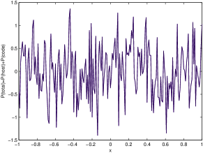
Figure 2: ”Chaotic” Nature of the Total Pdf, Eq. (16)

Acknowledgements

This work was supported by RAND-MSR contract CSM-DI $\ \&$ S-QIT-101107-2005. Gratitude is expressed to B. R. Frieden, A. Plastino, and, B. Soffer for helpful discussions.

References

• [1] L. D. Landau and E. M. Lifshitz. Quantum Mechanics. 3rd edn, Pergamon Press, Oxford, 1977.
• [2] B. R. Frieden. Science from Fisher Information: A Unification. Cambridge University Press, Cambridge. 2004.
• [3] R.  C. Venkatesan. Encryption of Covert Information into Multiple Statistical Distributions. Phys. lett. A, To Appear. Preprint available at at http://arxiv.org/abs/cond-mat/0607454, 2007.
• [4] B. Schneier. Applied Cryptography. 2nd edn., John Wiley $\ \&$ Sons, New York, NY, 1996.
• [5] R. L. Rivest. Cryptography and Machine Learning. Proceedings ASIACRYPT ’91, 2006, pp.427-439, Springer 1993. Article available at http://theory.lcs.mit.edu/ rivest/Rivest-CryptographyAndMachineLearning.pdf.
• [6] T. Cover and J. Thomas. Elements of Information Theory. John Wiley $\ \&$ Sons, New York, NY, 1991.
• [7] P. J. Hüber. Robust Statistics. John Wiley $\ \&$ Sons, New York, NY, 1981.
• [8] D. Horn and A. Gottlieb. Algorithm for Data Clustering in Pattern Recognition Problems based on Quantum Mechanics. Phys. Rev. Lett., 88, pp 18702(1)-18702(4), 2006.
• [9] R. C. Venkatesan. Encryption of Covert Information through a Fisher Game. In Exploratory Data Analysis Using Fisher Information, Frieden, B.R. and Gatenby, R.A., (Eds.), Springer-Verlag, London, pp. 181-216, 2006.
• [10] P. A. M. Dirac. Principles of Quantum Mechanics (The International Series of Monographs on Physics). Oxford University Press, Oxford, 1982.
• [11] H. L. van Trees. Detection, Estimation, and Modulation Theory, Part I,. Wiley, New York, NY, 1968.
• [12] M. S. Rogalski and S. B. Palmer. Quantum Physics. Gordon $\ \&$ Breach Science Publications, Amsterdam, The Netherlands, 1998.
• [13] A, Puente, M. Casas, and A. Plastino. Fisher Information and Semiclassical Methods. Phys. Rev. A, 59(5), pp 3211-3217, 1999.
• [14] L. Brillouin. Science and Information Theory. Academic Press, New York, NY, 1956.
• [15] O. Morgenstern and J. von Neumann. Theory of Games and Economic Behavior. Princeton University Press, Princeton, NJ, 1947.
• [16] G. Gigerenzer and R. Selten. Bounded Rationality. The MIT Press, Cambridge, MA, 2002.
• [17] David Wolpert. Information Theory - The Bridge Connecting Bounded Rational Game Theory and Statistical Physics. Complex Engineering Systems, Braha D. and Bar-Yam Y. (Eds.), Perseus Books, Boston, MA, 2004. Article available at http://arxiv.org/abs/cond-mat/0402508.
• [18] G. H. Golub and C. F. van Loan. Matrix Computations. 3rd edn, Johns Hopkins University Press, Baltimore, MD, 1995.
• [19] M. A. Nielsen and I. L. Chuang. Quantum Computation and Quantum Information. Cambridge University Press, Cambridge, 2000.