Coherent spectral weights of Gutzwiller-projected superconductors

Abstract

We analyze the electronic Green’s functions in the superconducting ground state of the $t$-$J$ model using Gutzwiller-projected wave functions, and compare them to the conventional BCS form. Some of the properties of the BCS state are preserved by the projection: the total spectral weight is continuous around the quasiparticle node and approximately constant along the Fermi surface. On the other hand, the overall spectral weight is reduced by the projection with a momentum-dependent renormalization, and the projection produces electron-hole asymmetry in renormalization of the electron and hole spectral weights. The latter asymmetry leads to the bending of the effective Fermi surface which we define as the locus of equal electron and hole spectral weight.

1 Introduction

High temperature superconductivity (HTSC) is one of the most intriguing phenomena in modern solid state physics. Experimentally, HTSC is observed in layered cuprate compounds. The undoped cuprates are antiferromagnetically ordered insulators which develop the characteristic superconducting “dome” upon doping with charge carriers.

HTSC is interesting not only for promising technological applications, but also from a theoretical point of view. The relevant ingredients for HTSC are believed to be the following.

• Low dimensionality (2d).

• Strong short-range repulsion between electrons.

• Doped Mott insulator.

Taking these 3 ingredients, HTSC is modeled in the tight-binding description by large-$U$ Hubbard models or $t$-$J$ models on the square lattice:

$$H_{tJ}=-t\sum_{\langle i,j\rangle}P_{G}\,c_{i\sigma}^{\dagger}c_{j\sigma}\,P_{G}+J\sum_{\langle i,j\rangle}({\bm{S}}_{i}\cdot{\bm{S}}_{j}-\frac{n_{i}n_{j}}{4})$$ (1)

where $n=c_{\sigma}^{\dagger}c_{\sigma}$, ${\bm{S}}=\frac{1}{2}c_{\sigma}^{\dagger}\bm{\sigma}_{\sigma\sigma^{\prime}}c_{\sigma^{\prime}}$ and $\bm{\sigma}$ are the Pauli matrices. The Gutzwiller projector $P_{G}=\Pi_{i}(1-n_{i\uparrow}n_{i\downarrow})$ prevents electrons from occupying the same lattice site.

The non-perturbative nature of the $t$-$J$ model makes it an outstanding problem to solve in dimensions larger than one. Analytical techniques (renormalized or slave-boson mean-field theories rmft ; kotliar88 ) are very crude and numerical techniques (e.g. exact diagonalization or cluster DMFT) are restricted to very small clusters or infinite dimensions, or they fail on the sign problem (QMC). An alternative approach was suggested by Anderson shortly after the experimental discovery of HTSC, when he proposed a Gutzwiller-projected BCS wave function as superconducting ground state for cuprates anderson87 . Following this conjecture, many variational studies have been performed on the basis of what is called Anderson’s (long range) RVB state. This state turned out to have very low variational energy, close to exact ground state energies, as well as high overlap with the true ground states of small $t$-$J$ clusters gros88 ; hasegawa89 . On the other hand, many experimental facts about cuprate superconductors can be reproduced and are consistent with the variational results: e.g. clearly favored $d$-wave pairing symmetry, doping dependency of the nodal Fermi velocity and the nodal quasiparticle weight. Many of these successful efforts following Anderson’s proposal are summarized in the “plain vanilla RVB theory” of HTSC, recently reviewed in anderson04 .

With help of the relatively recent technique of angle-resolved photoemission spectroscopy (ARPES), experimentalists can probe the electronic structure of low-lying excitations inside the copper planes. The intensity measured in ARPES is proportional to the one–particle electronic spectral function: $I_{PES}({\bm{k}},\omega)\;\propto A({\bm{k}},\omega)$ ARPES . It is therefore interesting to explore spectral properties within the framework of Gutzwiller-projected variational quasiparticle (QP) excitations.

In this contribution we will discuss some of our results reported in bieri06 . For more details, in particular for more reference to experimental studies, we invite the reader to consult that paper.

2 Coherent spectral weights

Anderson’s RVB state is given by

$$|H\rangle\propto P_{H}P_{G}|d\text{BCS}(\Delta,\mu)\rangle\;.$$ (2)

We further define projected BCS quasiparticle excitations in a similar way,

$$|H,\bm{k},\sigma\rangle\propto P_{H}P_{G}\gamma^{\dagger}_{\bm{k}\sigma}|d\text{BCS}\rangle\;.$$ (3)

The unprojected states in Eqs. (2) and (3) are the usual ingredients of the BCS theory, $|d\text{BCS}\rangle=\Pi_{\bm{k},\sigma}\gamma_{\bm{k}\sigma}|0\rangle$, $\gamma_{\bm{k}\sigma}=u_{\bm{k}}c_{\bm{k}\sigma}+{\small\sigma}v_{\bm{k}}c_{-\bm{k}\bar{\sigma}}^{\dagger}$, $u_{\bm{k}}^{2}=\frac{1}{2}\left(1-\frac{\xi_{\bm{k}}}{E_{\bm{k}}}\right)=1-v_{\bm{k}}^{2}$, $E_{\bm{k}}=\sqrt{\xi_{\bm{k}}^{2}+\Delta_{\bm{k}}^{2}}$, $\xi_{\bm{k}}=-2[\cos(k_{x})+\cos(k_{y})]-\mu$, $\Delta_{\bm{k}}=\Delta[\cos(k_{x})-\cos(k_{y})]$. $P_{G}$ is the Gutzwiller projector and $P_{H}$ projects on the subspace with $H$ holes. $|H\rangle$ and $|H,\bm{k},\sigma\rangle$ are normalized to one. The wave functions have two variational parameters, $\Delta$ and $\mu$, which we adjusted to minimize the energy of the $t$-$J$ Hamiltonian (1) for the experimentally relevant value $J=0.3$ and every doping level. Note that in the RVB theory, $\Delta$ and $\mu$ are variational parameters without direct physical significance; physical quantities like excitation gap, superconducting order, or chemical potential must be calculated explicitly.

The spectral weights of the coherent low-lying quasiparticles (3) can be written as

$$Z^{+}_{\bm{k}}= |\langle H-1,\bm{k},\sigma|c_{{\bm{k}},\sigma}^{\dagger}|H\rangle|^{2}$$ (4a)

$$Z^{-}_{\bm{k}}= |\langle H+1,\bm{k},\sigma|c_{-{\bm{k}},\bar{\sigma}}|H\rangle|^{2}\;.$$ (4b)

These weights are measured in ARPES experiments as the residues of the spectral function $A({\bm{k}},\omega)$ ARPES . Note that in conventional BCS-theory, $Z_{\bf k}^{+}=u_{\bm{k}}^{2}$ and $Z_{\bf k}^{-}=v_{\bm{k}}^{2}$.

3 Method: VMC

The variational Monte Carlo technique (VMC) allows to evaluate fermionic expectation values of the form $\langle\psi|O|\psi\rangle$ for a given state $|\psi\rangle$. In order to calculate the spectral weights (4) by VMC, the following exact relations can be used.

$$Z^{+}_{\bm{k}} = \frac{1+x}{2}-\langle c^{\dagger}_{\bm{k}\sigma}c_{\bm{k}\sigma}\rangle\;,$$ (5a)

$$Z^{+}_{\bm{k}}Z^{-}_{\bm{k}} = \lvert\langle H+1|c_{\bm{k}\uparrow}c_{-\bm{k}\downarrow}|H-1\rangle\rvert^{2}\;,$$ (5b)

where $x$ is hole doping yunoki05 ; bieri06 .

We use VMC to calculate the superconducting order parameter $\Phi_{\bm{k}}=\lvert\langle c_{\bm{k}\uparrow}c_{-\bm{k}\downarrow}\rangle\rvert$, as well as diagonal matrix elements in the optimized $t$-$J$ ground state (2). Using relations (5), we can then derive the spectral weights (4). The disadvantage of this procedure is large errorbars around the center of the Brillouin zone where both $Z^{+}_{\bm{k}}$ and $\Phi_{\bm{k}}$ are small.

4 Results

In Fig. 1, we plot the nearest-neighbor superconducting orderparameter $\langle c_{i\uparrow}c_{j\downarrow}\rangle$ as a function of doping. The curve shows close quantitative agreement with the result of Ref. paramekanti0103 , where the authors extracted the same quantity from the long-range asymptotics of the nearest-neighbor pairing correlator, $\lim_{r\rightarrow\infty}\langle c_{0}c_{\delta}c^{\dagger}_{r}c_{r+\delta}^{\dagger}\rangle$. With the method employed here, we find the same qualitative and quantitative conclusions of previous authors gros88 ; paramekanti0103 : vanishing of superconductivity at half filling, $x\to 0$, and at the superconducting transition on the overdoped side, $x_{c}\simeq 0.3$. The optimal doping is near $x_{opt}\simeq 0.18$. In the same plot we also show the commonly used Gutzwiller approximation where the BCS orderparameter is renormalized by the factor $g_{t}=\frac{2x}{1+x}$ rmft . The Gutzwiller approximation underestimates the exact value by approximately $25\%$.

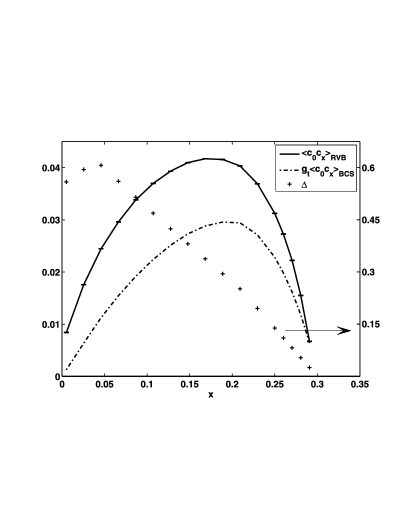
Figure 1: Doping dependency of the nearest-neighbor superconducting order parameter $\Phi_{ij}$ (calculated in the 14$\times 14$ system). The errorbars are smaller than the symbol size. The same quantity calculated in the Gutzwiller approximation is also shown for comparison. The variational parameter $\Delta$ is shown with the scale on the right.

In Fig. 2, we plot the spectral weights $Z^{+}_{\bm{k}}$, $Z^{-}_{\bm{k}}$, and $Z^{tot}_{\bm{k}}$ along the contour $0\to(0,\pi)\to(\pi,\pi)\to 0$ in the Brillouin zone for different doping levels. Figure 3 shows the contour plots of $Z^{tot}_{\bm{k}}$ in the region of the Brillouin zone where our method produces small errorbars. From these data, we can make the following observations.

• In the case of an unprojected BCS wave function, the total spectral weight is constant and unity over the Brillouin zone. Introducing the projection operator, we see that for low doping ($x\simeq 3\%$), the spectral weight is reduced by a factor up to $20$. The renormalization is asymmetric in the sense that the electronic spectral weight $Z^{+}_{\bm{k}}$ is more reduced than the hole spectral weight $Z^{-}_{\bm{k}}$. For higher doping ($x\simeq 23\%$), the spectral weight reduction is much smaller and the electron-hole asymmetry decreases.

• Since there is no electron-hole mixing along the zone diagonal ($d$-wave), the spectral weights $Z^{+}_{\bm{k}}$ and $Z^{-}_{\bm{k}}$ have a discontinuity at the nodal point. Our data shows that the total spectral weight is continuous across the nodal point. Strong correlation does not affect these features of uncorrelated BCS-theory.

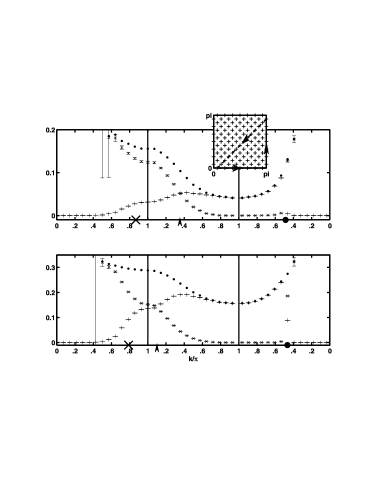
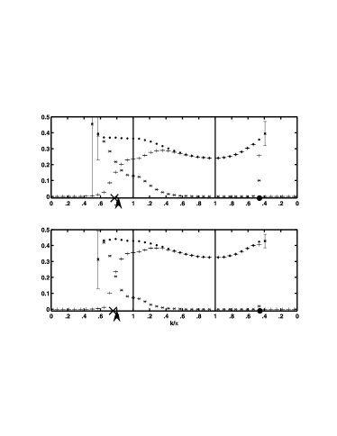
Figure 2: QP spectral weights for 6 holes (upper left plot, $x\simeq 3\%$), 22 holes (lower left plot, $x\simeq 11\%$), 34 holes (upper right plot, $x\simeq 17\%$), and 46 holes (lower right plot, $x\simeq 23\%$) on 196 sites. The spectral weights are plotted along the contour $0\to(0,\pi)\to(\pi,\pi)\to 0$ (shown in inset). Plus signs ($+$) denote the spectral weight $Z_{\bm{k}}^{+}$, crosses ($\times$) denote $Z_{\bm{k}}^{-}$, errorbars are shown. Solid dots denote their sum, the total spectral weight $Z_{\bm{k}}^{tot}$, errorbars not shown. On the horizontal axis, the star ($*$) denotes the intersection with the unprojected Fermi surface along the $0\to(0,\pi)$ direction; the thick dot is the nodal point. Both $Z_{\bm{k}}^{+}$ and $Z_{\bm{k}}^{-}$ jump at the nodal point, while $Z_{\bm{k}}^{tot}$ is continuous. The intersection with the effective Fermi surface (see text) is marked by an arrowhead. On the diagonal (last segment), $k/\pi$ is given in units of $\sqrt{2}$.

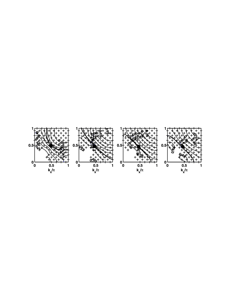
Figure 3: Contour plots of the total QP spectral weight $Z_{\bm{k}}^{tot}$. The effective FS (full line) and unprojected FS (dashed line) are also shown. The doping levels are $x\simeq 3\%$, $11\%$, $17\%$, and $23\%$ (from left to right). The $+$ signs indicate points where the values are known within small errorbars (see Section Method: VMC).

4.1 Effective Fermi surface

In strongly interacting Fermi systems, the notion of a Fermi surface (FS) is not clear at all. There are, however, several experimental definitions of the FS. Most commonly, ${\bm{k}}_{F}$ is determined in ARPES experiments as the maximum of $|{\bm{\nabla}}_{\bm{k}}n_{\bm{k}}|$ or the locus of minimal gap along some cut in the $\bm{k}$-plane. The theoretically better defined locus of $n_{\bm{k}}=1/2$ is also sometimes used. The various definitions of the FS usually agree within the experimental uncertainties ARPES . The different definitions of the FS in HTSC were recently analyzed theoretically in Refs. gros06 ; sensarma06 .

Here, we propose an alternative definition of the Fermi surface based on the ground state equal-time Green’s functions. In the unprojected BCS state, the underlying FS is determined by the condition $|u_{\bm{k}}|^{2}=|v_{\bm{k}}|^{2}$. We will refer to this as the unprojected FS. Since $|u_{\bm{k}}|^{2}$ and $|v_{\bm{k}}|^{2}$ are the residues of the QP poles in the BCS theory, it is natural to replace them in the interacting case by $Z^{+}_{\bm{k}}$ and $Z^{-}_{\bm{k}}$, respectively. We will therefore define the effective FS as the locus $Z^{+}_{\bm{k}}=Z^{-}_{\bm{k}}$.

In Fig. 3, we plot the unprojected and the effective FS which we obtained from VMC calculations. The contour plot of the total QP weight is also shown. It is interesting to note the following points.

• In the underdoped region, the effective FS is open and bent outwards (hole-like FS). In the overdoped region, the effective FS closes and embraces more and more the unprojected one as doping is increased (electron-like FS).

• Luttinger’s rule luttinger61 is clearly violated in the underdoped region, i.e. the area enclosed by the effective FS is not conserved by the interaction; it is larger than that of the unprojected FS.

• In the optimally doped and overdoped region, the total spectral weight is approximately constant along the effective FS within errorbars. In the highly underdoped region, we observe a small concentration of the spectral weight around the nodal point ($\simeq 20\%$).

Large “hole-like” FS in underdoped cuprates has also been reported in ARPES experiments by several groups ino04 ; yoshida03 ; shen03 .

It should be noted that a negative next-nearest hopping $t^{\prime}$ would lead to a similar FS curvature as we find in the underdoped region. We would like to emphasize that our original $t$-$J$ Hamiltonian as well as the variational states do not contain any $t^{\prime}$. Our results show that the outward curvature of the FS is due to strong repulsion, without need of $t^{\prime}$. The next-nearest hopping terms in the microscopic description of the cuprates may not be necessary to explain the FS topology found in ARPES experiments. Remarkably, if the next-nearest hopping $t^{\prime}$ is included in the variational ansatz (and not in the original $t$-$J$ Hamiltonian), a finite and negative $t^{\prime}$ is generated, as it was shown in Ref. himeda00 . Apparently, in this case the unprojected FS has the tendency to adjust to the effective FS. A similar bending of the FS was also reported in the recent analysis of the current carried by Gutzwiller-projected QPs nave06 . A high-temperature expansion of the momentum distribution function $n_{\bm{k}}$ of the $t$-$J$ model was done in Ref. putikka98 where the authors find a violation of Luttinger’s rule and a negative curvature of the FS. Our findings provide further evidence in this direction.

A natural question is the role of superconductivity in the unconventional bending of the FS. In the limit $\Delta\to 0$, the variational states are Gutzwiller-projected excitations of the Fermi sea and the spectral weights are step-functions at the (unprojected) FS. In a recent paper yang06 , it was shown that $\lim_{{\bm{k}}\rightarrow{\bm{k}}^{+}_{F}}Z^{+}_{\bm{k}}=\lim_{{\bm{k}}\rightarrow{\bm{k}}^{-}_{F}}Z^{-}_{\bm{k}}$ for the projected Fermi-sea, which means that the unprojected and the effective FS coincide in that case. This suggests that the “hole-like” FS results from a non-trivial interplay between strong correlation and superconductivity. At the moment, we lack a qualitative explanation of this effect. However, it may be a consequence of the proximity of the system to the non-superconducting “staggered-flux” state lee00 ; ivanov03 or to antiferromagnetism near half-filling paramekanti0103 ; ivanov06 .

5 Acknowledgement

SB would like to thank the organizers of the Eleventh Training Course in the Physics of Correlated Electron Systems and HTSC in Salerno, Italy, where this work was presented. We would like to thank George Jackeli for many illuminating discussions and continuous support. We also thank Claudius Gros, Patrick Lee, and Seiji Yunoki for interesting discussions. This work was supported by the Swiss National Science Foundation.

References

- (1)
- (2) F. C. Zhang, C. Gros, T. M. Rice, and H. Shiba, Supercond. Sci. Technol. 1, 36 (1988).
- (3) G. Kotliar and J. Liu, Phys. Rev. B 38, 5142 (1988).
- (4) P. W. Anderson, Science 235, 1196 (1987).
- (5) C. Gros, Phys. Rev. B 38, 931 (1988); Ann. Phys. (N.Y.) 189, 53 (1989).
- (6) Y. Hasegawa and D. Poilblanc, Phys. Rev. B 40, 9035 (1989).
- (7) P. W. Anderson, P. A. Lee, M. Randeria, M. Rice, N. Trivedi, and F. C. Zhang, J. Phys.: Condens. Matter 16, R755 (2004).
- (8) A. Damascelli, Z. Hussain, and Z.-X. Shen, Rev. Mod. Phys. 75, 473 (2003); J. C. Campuzano, M. R. Norman, and M. Randeria, in Physics of Superconductors, edited by K. H. Bennemann and J. B. Ketterson (Springer, Berlin, 2004), Vol. II, pp. 167-273; cond-mat/0209476.
- (9) S. Bieri and D. Ivanov, Phys. Rev. B. 75 035104 (2007); cond-mat/0606633.
- (10) S. Yunoki, Phys. Rev. B 72, 092505 (2005); Phys. Rev. B 74, 180504 (2006).
- (11) A. Paramekanti, M. Randeria, and N. Trivedi, Phys. Rev. Lett. 87, 217002 (2001); Phys. Rev. B 70, 054504 (2004).
- (12) C. Gros, B. Edegger, V. N. Muthukumar, and P. W. Anderson, Proc. Natl. Acad. Sci. U.S.A 103, 14298 (2006); cond-mat/0606750.
- (13) R. Sensarma, M. Randeria, and N. Trivedi, cond-mat/0607006.
- (14) J. M. Luttinger, Phys. Rev. 121, 942 (1961).
- (15) A. Ino, C. Kim, M. Nakamura, T. Yoshida, T. Mizokawa, A. Fujimori, Z.-X. Shen, T. Kakeshita, H. Eisaki, and S. Uchida, Phys. Rev. B 65, 094504 (2002).
- (16) T. Yoshida, X. J. Zhou, T. Sasagawa, W. L. Yang, P. V. Bogdanov, A. Lanzara, Z. Hussain, T. Mizokawa, A. Fujimori, H. Eisaki, Z.-X. Shen, T. Kakeshita, and S. Uchida, Phys. Rev. Lett. 91, 027001 (2003).
- (17) K. M. Shen, F. Ronning, D. H. Lu, F. Baumberger, N. J. C. Ingle, W. S. Lee, W. Meevasana, Y. Kohsaka, M. Azuma, M. Takano, and Z.-X. Shen, Science 307, 901 (2005).
- (18) A. Himeda and M. Ogata, Phys. Rev. Lett. 85, 4345 (2000).
- (19) C. P. Nave, D. A. Ivanov, and P. A. Lee, Phys. Rev. B 73, 104502 (2006).
- (20) W. O. Putikka, M. U. Luchini, and R. R. P. Singh, Phys. Rev. Lett. 81, 2966 (1998).
- (21) H. Yang, F. Yang, Y.-J. Jiang, and T. Li, cond-mat/0604488.
- (22) P. A. Lee and X.-G. Wen, Phys. Rev. B 63, 224517 (2000).
- (23) D. A. Ivanov and P. A. Lee, Phys. Rev. B 68, 132501 (2003).
- (24) D. A. Ivanov, Phys. Rev. B 74, 24525 (2006).