Extreme fluctuations in noisy task-completion landscapes on scale-free networks

Abstract

We study the statistics and scaling of extreme fluctuations in noisy task-completion landscapes, such as those emerging in synchronized distributed-computing networks, or generic causally-constrained queuing networks, with scale-free topology. In these networks the average size of the fluctuations becomes finite (synchronized state) and the extreme fluctuations typically diverge only logarithmically in the large system-size limit ensuring synchronization in a practical sense. Provided that local fluctuations in the network are short-tailed, the statistics of the extremes are governed by the Gumbel distribution. We present large-scale simulation results using the exact algorithmic rules, supported by mean-field arguments based on a coarse-grained description.

The understanding of the characteristics of fluctuations in task-completion landscapes in distributed processing networks is important from both fundamental and system-design viewpoints. Here, we study the statistics and scaling of the extreme fluctuations in synchronization landscapes of task-completion networks with scale-free topology. These systems have a large number of coupled components and the tasks performed on each component (node) evolve according to the local synchronization scheme. We consider short-tailed local stochastic task-increments, motivated by certain distributed-computing algorithms implemented on networks. In essence, in order to perform certain tasks, processing nodes in the network must often wait for others, since their assigned task may need the output of other nodes. Typically, large fluctuations in these networks are to be avoided for performance reasons. Understanding the statistics of the extreme fluctuations in our model, will help us to better understand the generic features of back-log formations and worst-case delays in networked processing systems. We find that the average size of the fluctuations in the associated landscape on scale-free networks becomes finite and largest fluctuations diverge only logarithmically in the large system-size limit. This weak divergence ensures an autonomously-synchronized, near-uniform progress in the distributed processing network. The statistics of the maximum fluctuations on the landscape is governed by the Gumbel distribution.

I Introduction

Many artificial and natural systems can be described by models of complex networks Boccaletti et al. (2006); Newman (2003); Dorogovtsev and Mendes (2002); Albert and Barabási (2002); Bollobás (2001). The ubiquity of complex networks has led to a dramatic increase in the study of the structure of these systems. Recent research on networks has shifted the focus from the structural (topological) analysis to the study of processes (dynamics) in these complex interconnected systems. The main problem addressed in these studies is how the underlying network topology influences the collective behavior of the system.

Synchronization is a good example for processes in networks and it is also a fundamental problem in natural and artificial coupled multi-component systems Strogatz (2001). Since the introduction of small-world (SW) networks Watts and Strogatz (1998); Watts (1999), it has been established that such networks can facilitate autonomous synchronization Barahona and Pecora (2002); Wang and Chen (2002a); Hong et al. (2002). Synchronization in the context of coupled nonlinear dynamical systems such as chaotic oscillators has been also studied in scale-free networks Wang and Chen (2002b); Nishikawa et al. (2003); Motter et al. (2005a, b); Zhou et al. (2006); Zhou and Kurths (2006). In these studies the ratio of the largest and the smallest non-zero eigenvalues of the network Laplacian (in the linearized problem) has been used as a measure for “desynchronization”, i.e., smaller ratios corresponding to better synchronizability.

Another synchronization problem emerges in the context of parallel discrete-event simulations Lubachevsky (1988); Korniss et al. (2000); Sloot et al. (2001); Korniss et al. (2003); Kirkpatrick (2003); Kolakowska and Novotny (2005). Nodes must frequently “synchronize” with their neighbors (on a given network) to ensure causality in the underlying simulated dynamics. The local synchronizations, however, can introduce correlations in the resulting task-completion landscape, leading to strongly non-uniform progress at the individual processing nodes. The above is a prototypical example for task-completion landscapes in causally-constrained queuing networks Toroczkai et al. (2006). Analogous questions can also be posed in supply-chain networks based on electronic transactions Nagurney et al. (2005) etc. The basic task-completion model has been considered for regular (in 1D Korniss et al. (2000, 2001, 2002) and 2D Guclu et al. (2006); Guclu (2005)), small-world Korniss et al. (2003) and scale-free (SF) networks Toroczkai et al. (2006); Guclu (2005); Korniss (2006). The extreme fluctuations in SW networks also have been studied Guclu et al. (2004); Guclu and Korniss (2005) previously. Here, we provide a detailed account and new results on the extreme fluctuations in task-completion networks with SF structure. Through our study, one also gains some insight into the effects of SF interaction topologies on the suppression of critical fluctuations in interacting system.

The field of extremes has attracted the attention of engineers, scientists, mathematicians and statisticians for many years. From an engineering point of view, physical structures need to be designed such that special attention is paid to properties under extreme conditions requiring an understanding of the statistics of extremes (minima and maxima) in addition to average values. Fisher and Tippett (1928); Gumbel (1958); Galambos (1987). For example, in designing a dam, engineers, in addition to being interested in average flood, which gives the total amount of water to be stored, are also interested in the maximum flood, the maximum earthquake intensity or the minimum strength of the concrete used in building the dam Castillo et al. (2005). Extreme-value theory is unique as a statistical discipline in that it develops techniques and models for describing the unusual rather than the usual Coles (2001). Similarly, in networked processing systems, in addition to the average “load” or progress, knowing the typical size and the distribution of the extreme fluctuations is of great importance, since failures and delays are triggered by extreme events occurring on an individual node or link.

The relationship between extremal statistics and universal fluctuations of global order parameters in correlated systems has been the subject of recent intense research Bramwell et al. (1998, 2000); Watkins et al. (2002); Bramwell et al. (2002, 2001); Aji and Goldenfeld (2001); Antal et al. (2001, 2002); Dahlstedt and Jensen (2001); Chapman et al. (2002); Györgyi et al. (2003); Bouchaud and Mézard (1997); Baldassarri et al. (2002); Bertin (2005). Closer to our interest, universal distributions for explicitly the extreme “height” fluctuations have been studied for fluctuating surfaces Raychaudhuri et al. (2001); Majumdar and Comtet (2004, 2005); Kearney and Majumdar (2005); Schehr and Majumdar (2006); Györgyi et al. (2006), in particular for the Kardar-Parisi-Zhang (KPZ) surface growth model Kardar et al. (1986) in one dimension Majumdar and Comtet (2004, 2005). It turns out that the basic task-completion landscape (emerging in certain synchronized distributed computing schemes), on regular lattices, belongs precisely to the KPZ universality class Korniss et al. (2000); Guclu et al. (2006). In this paper, we address the suppression of the extreme fluctuations of the local order parameter (local progress) in scale-free (SF) noisy task-completion networks.

This paper is organized as follows. In Section II we give a brief review on the extreme-value statistics of independent and identically-distributed random variables, with some further details for exponential-like random variables. Section III describes our prototypical model for task-completion systems and provides a mathematical framework to analyze the evolution of its progress landscape. We present our results in Section IV and finish the paper with conclusions and summary in Section V.

II Extreme-Value Statistics

Extreme-value theory deals with stochastic behavior of the maxima and minima of random variables. Let us first focus on independent and identically distributed (iid) random variables. The distributional properties of the extremes are determined by the tails of the underlying individual distributions. By definition extreme values are scarce implying an extrapolation from observed levels to unobserved levels, and extreme value theory provides a class of models to enable such extrapolation Coles (2001).

Historically, work on extreme value problems may be traced back to as early as 1700s when Bernoulli discussed the mean largest distance from the origin given some points lying at random on a straight line of a fixed length (See Gumbel (1958)). Theoretical developments of extreme-value statistics in 1920s von Bortkiewicz (1922); von Mises (1923); Dodd (1923); Frechét (1927); Fisher and Tippett (1928) were followed by research dealing with practical applications in radioactive emissions Gumbel (1937), flood analysis Gumbel (1941), strength of materials Weibull (1939), seismic analysis Nordquist (1945), rainfall analysis Potter (1959) etc. In terms of applications, Gumbel Gumbel (1958), made several contributions to extreme value analysis and called the attention of engineers and statisticians to applications of the extreme-value theory. Here, we review Kotz and Nadarajah (2000) the basics on the statistics of the maximum of $N$ iid random variables.

Let $X$ be a random variable with probability density function (pdf) $f(x)$ and cumulative distribution function (cdf) $F(x)$ (the probability that the individual stochastic variable is less than $x$). $f(x)$ and $F(x)$ are also referred to as the parent distributions. Let $\{X_{i}\}_{i=1}^{N}$ be an iid sample drawn from $f(x)$. Then the joint pdf can be written as

$$f(X_{1},X_{2},...,X_{N})=\prod_{i=1}^{N}f(X_{i})\;,$$ (1)

and their joint cdf as

$$F(X_{1},X_{2},...,X_{N})=\prod_{i=1}^{N}F(X_{i})\;.$$ (2)

Then the cdf of the maximum order statistic, $X_{M}=\max\{X_{1},X_{2},...,X_{N}\}$, for iid random variables, can be written as

$$F_{M}(x) = {\rm Pr}(X_{M}\leq x)$$ (3)

$$= {\rm Pr}(\text{max}\{X_{1},X_{2},...,X_{N}\}\leq x)$$

$$= {\rm Pr}(X_{1}\leq x;X_{2}\leq x;\ldots;X_{N}\leq x;)$$

$$= \prod_{i=1}^{N}{\rm Pr}(X_{i}\leq x)=\prod_{i=1}^{N}F(x)=[F(x)]^{N}\;.$$

The pdf of $X_{M}$ can be calculated by differentiating the equation above with respect to $x$, yielding

$$f_{M}(x)=Nf(x)[F(x)]^{N-1}\;.$$ (4)

In many situations, extreme value analysis is built on a sequence of data that is block (sample) maxima or minima. A traditional discussion on the mean of the sample is based on the central limit theorem and it forms the basis for statistical inference theory Beirlant et al. (2004). The central limit theorem deals with the statistics of the sum $S_{N}$$=$$X_{1}+X_{2}+...+X_{N}$ (proportional to the arithmetic average) and provides the constants $a_{N}$ and $b_{N}$$>$$0$ such that $Y_{N}$$=$$(S_{N}-a_{N})/b_{N}$ tends in distribution to a non-degenerate distribution. In the case when $X$ has finite variance, this distribution is the normal distribution. However, when the underlying distribution has a slowly decaying (or heavy) tail, some other stable distributions are attained instead of normal distribution Bouchaud (2000). Specifically, power-law distributions with infinite variance will yield non-normal limits for the average: the extremes produced by such a sample will “corrupt” the average so that an asymptotic behavior different from the normal behavior is obtained Beirlant et al. (2004).

As the sample size $N$ goes to infinity, it is clear that for any fixed value of $x$ the distribution of the maxima becomes

$$\lim_{N\rightarrow\infty}F_{M}(x)=\left\{\begin{array}[]{ll}1&\text{if}~{}F(x)=1\\ 0&\text{if}~{}F(x)<1\\ \end{array}\right.\;,$$ (5)

which is a degenerate distribution (it takes the values $0$ and $1$ only). If there is a limiting distribution, one has to obtain it in terms of a sequence of transformed (or reduced) variable, such as $(X_{M}-a_{N})/b_{N}$ where $a_{N}$ and $b_{N}(>0)$ may depend on $N$ but not $x$. The main mathematical challenge here is finding the sequence of numbers ($a_{N}$ and $b_{N}$) such that for all real values of $x$ (at which the limit is continuous) the limit goes to a non-degenerate distribution.

$$Pr(\frac{X_{M}-a_{N}}{b_{N}}\leq x)\rightarrow G_{M}(x)~{}\text{as}~{}N\rightarrow\infty\;.$$ (6)

The problem is twofold: (i) finding all possible (non-degenerate) distributions G that can appear as a limit in Eq. (6); (ii) characterizing the distributions F for which there exist sequences $\{a_{N}\}$ and $\{b_{N}\}$ such that Eq. (6) holds for any such specific limit distribution Beirlant et al. (2004). The first problem is the (extremal) limit problem and has been solved in Frechét (1927); Fisher and Tippett (1928); Gnedenko (1943) and later revived in de Haan (1970). The second part of the problem is called the domain of attraction problem. Under the transformation through $a_{N}$ and $b_{N}$ the extreme types theorem states that the non-degenerate distribution $G_{M}$ belongs to one of the following families

$$G_{M}(x)=\left\{\begin{array}[]{ll}\exp[-\exp(\frac{\lambda-x}{\sigma})],&-\infty<x<\infty\\ \end{array}\right.\;,$$ (7)

$$G_{M}(x)=\left\{\begin{array}[]{ll}0,&\text{if}~{}x<\lambda\\ \exp[-(\frac{\sigma}{x-\lambda})^{\omega}],&\text{otherwise}\\ \end{array}\right.\;,$$ (8)

$$G_{M}(x)=\left\{\begin{array}[]{ll}\exp[-(\frac{\lambda-x}{\sigma})^{\omega}],&\text{if}~{}x<\lambda\\ 1,&\text{otherwise}\\ \end{array}\right.\;.$$ (9)

Collectively, these three classes of distributions are widely known as Gumbel, Fréchet and Weibull distributions, respectively. Each family has a location and a scale parameter, $\lambda$ and $\sigma$, respectively; additionally, the Fréchet and Weibull families have a shape parameter $\omega$. The above theorem implies that when $X_{M}$ can be stabilized with suitable sequences $a_{N}$ and $b_{N}$, the corresponding normalized variable $X_{M}^{*}$$=$$(X_{M}$$-$$a_{N})$$/$$b_{N}$ has a limiting distribution that must be one of the three types of extreme value distribution. The remarkable feature of this result is that the three types of extreme-value distributions are the only possible limits for the distributions of the $X_{M}^{*}$, regardless of the parent distribution $F$ for the population. In this sense, the theorem is an extreme-value analog of the central limit theorem Coles (2001).

Table 1: Domain of attractions of the most common distributions for the maximum of iid random variables.

Distribution	Domain
Normal	Gumbel
Exponential	Gumbel
Lognormal	Gumbel
Gamma	Gumbel
Uniform	Weibull
Pareto	Fréchet

Now we briefly summarize, the basic properties for the maximal values of $N$ independent stochastic variables Fisher and Tippett (1928); Gumbel (1958); Galambos (1987); Baldassarri (2000); Bouchaud and Mézard (1997) drawn from a generic exponential-like individual pdf. We consider the case when the parent complementary cdf (survival function), $S(x)$$=$$1$$-$$F(x)$, (the probability that the individual stochastic variable is larger than $x$) decays faster than any power law in the tail, i.e., exhibits an exponential-like tail in the large-$x$ limit. (Note that in this case the corresponding probability density function displays the same exponential-like asymptotic tail behavior.) Using Eq. (3) the cumulative distribution $F_{M}(x)$ for the largest of the $N$ events (the probability that the maximum value is less than $x$) can be approximated as Bouchaud and Mézard (1997); Bouchaud (2000); Baldassarri (2000)

$$F_{M}(x)=[F(x)]^{N}=[1-S(x)]^{N}=e^{N\ln[1-S(x)]}\simeq e^{-NS(x)}\;,$$ (10)

where one typically assumes that the dominant contribution to the statistics of the maximum comes from the tail of the individual distribution. Now we assume $S(x)\simeq e^{-cx^{\delta}}$ for large $x$ values, where $c$ is a constant and $\delta$ characterizes the exponential-like tail. This yields

$$F_{M}(x)\simeq e^{-e^{-cx^{\delta}+\ln(N)}}.$$ (11)

The extreme-value limit theorem implies that there exists a sequence of scaled variables $\tilde{x}=(x-a_{N})/b_{N}$, such that in the limit of $N$$\to$$\infty$, the extreme-value probability distribution for $\tilde{x}$ asymptotically approaches the standard form of the Gumbel (also known as Fisher-Tippet Type I) distribution Fisher and Tippett (1928); Gumbel (1958):

$$G_{M}(\tilde{x})\simeq e^{-e^{-\tilde{x}}}\;,$$ (12)

with the corresponding pdf

$$g_{M}(\tilde{x})\simeq e^{-\tilde{x}-e^{-\tilde{x}}}\;,$$ (13)

with mean $\langle\tilde{x}\rangle$$=$$\gamma$ ($\gamma$$=$$0.577\ldots$ being the Euler constant) and variance $\sigma_{\tilde{x}}^{2}$$=$$\langle\tilde{x}^{2}\rangle$$-$$\langle\tilde{x}\rangle^{2}$$=$$\pi^{2}/6$. From Eqs. (11) and (12), one can deduce Baldassarri (2000) that to leading order, the scaling coefficients must be $a_{N}$$=$$[\ln(N)/c]^{1/\delta}$ and $b_{N}$$=$$(\delta c)^{-1}[\ln(N)/c]^{(1/\delta)-1}$. Note that for $\delta$$\neq$$1$, while the convergence to Eq. (11) is fast, the convergence for the appropriately scaled variable to the universal Gumbel distribution in Eq. (12) is extremely slow Fisher and Tippett (1928); Baldassarri (2000). The average value of the largest of the $N$ iid variables with an exponential-like tails then scales as

$$\langle x_{\max}\rangle=a_{N}+b_{N}\gamma\simeq[\ln(N)/c]^{1/\delta}$$ (14)

(up to ${\cal O}(\frac{1}{\ln(N)})$ corrections) in the asymptotic large-$N$ limit. When comparing with experimental or simulation data, instead of Eq. (12), it is often convenient to use the Gumbel distribution scaled to zero mean and unit variance, yielding

$$G_{M}(y)=e^{-e^{-(ay+\gamma)}}\;,$$ (15)

where $a$$=$$\pi/\sqrt{6}$ and $\gamma$ is the Euler constant. In particular, the corresponding Gumbel pdf becomes

$$g_{M}(y)=ae^{-(ay+\gamma)-e^{-(ay+\gamma)}}\;.$$ (16)

The mathematical arguments in obtaining the limit distributions above assume an underlying process consisting of a sequence of independent and identically distributed random variables. The most natural application of a sequence of independent random variables is to a stationary series. For some physical processes, stationarity is a reasonable assumption and corresponds to a series whose variables may be mutually dependent but whose stochastic properties are homogeneous in time. There, the main problem is finding the form of stationarity in terms of the range of dependence. Then one attempts to find the timescale of the series in which extreme events are almost independent. This is a strong assumption, but there are a number of empirical stationary series satisfying this property Eichner et al. (2006). Then, eliminating the long-range dependence of extremes provides an opportunity to consider only the effect of short-range (or weak) dependence by using some rigorous Galambos (1987); Berman (1964) or heuristic arguments leading to simple quantification in terms of the standard extreme-value limits.

In this paper we will not discuss in detail the basic formulation and treatment of the extreme limit distributions of dependent random variables. Detailed work on limit distributions and conditions required for different kinds of sequences such as Markov, m-dependent, moving average, normal sequences etc. can be found in the literature Coles (2001); Castillo et al. (2005). Most of the research focused on weakly correlated random variables Galambos (1987); Berman (1964) and only recent results have become available on the statistical properties of the extremes of strongly correlated variables Majumdar and Comtet (2004, 2005); Kearney and Majumdar (2005); Schehr and Majumdar (2006); Raychaudhuri et al. (2001); Györgyi et al. (2006). Traditional approaches, based on effectively uncorrelated variables, immediately break down. Only recently, Majumdar and Comtet Majumdar and Comtet (2004, 2005) obtained analytic results for the distribution of extreme-height fluctuations in the simplest strongly correlated fluctuating landscape: the steady state of the one dimensional surface-growth EW/KPZ model.

As it becomes apparent, in light of recent results on SW Guclu and Korniss (2004, 2005) and our new results on SF networks presented here (Sec. IV), implementing our stochastic nonlinear rules for the task-completion model on a complex interaction topology, in effect, “eliminates” the complexity of the task-completion landscape. While in low dimensions and regular topologies fluctuations are strongly correlated and “critical”, in that they are controlled by a diverging correlation length, on complex networks, correlations become weak (or mean-field like), and one expects the extreme fluctuations in the task-completion landscape to be effectively governed by the traditional extreme-value limit distributions for independent variables.

III Task-Completion Networks

III.1 The Model and Its Coarse-grained Description

Consider an arbitrary network in which the nodes interact through the links. The nodes are assumed to be task processing units, such as computers or manufacturing devices. Each node has completed an amount of tasks $\tau_{i}$ and these together (at all nodes) constitute the task-completion landscape $\{\tau_{i}(t)\}_{i=1}^{N}$. Here $t$ is the discrete number of parallel steps executed by all nodes, which is proportional to the real time and $N$ is the number of nodes. At each parallel step $t$, only certain nodes can receive additional tasks and when that happens we say that an update happened at those nodes. In this particular model the nodes that are allowed to update at a given step are those whose completed task amount is not greater than the tasks at their neighbors. We also choose the amount of new tasks arriving at a node to be a random variable distributed according to an exponential distribution (Poisson asynchrony). An example of a system being described by this model is a parallel computer simulating short-range correlated discrete events in continuous time with a Poisson inter-arrival time distribution between the events (independent events) Lubachevsky (1988); Korniss et al. (2000); Sloot et al. (2001); Korniss et al. (2003); Kirkpatrick (2003); Kolakowska and Novotny (2005). Thus, denoting the neighborhood of the node $i$ by $S_{i}$, if $\tau_{i}(t)\leq\min_{j\in S_{i}}\{\tau_{j}(t)\}$, the node $i$ completes some additional exponentially distributed random amount of task. Otherwise, it idles. In its simplest form the evolution equation for the amount of task completed at the node $i$ can be written

$$\tau_{i}(t+1)=\tau_{i}(t)+\eta_{i}(t)\prod_{j\in S(i)}\Theta\left(\tau_{j}(t)-\tau_{i}(t)\right)\;,$$ (17)

where $\tau_{i}$ is the local field variable (amount of task completed) at node $i$ at time $t$, $\eta_{i}(t)$ are identical, exponentially distributed random variables with unit mean, delta-correlated in space and time (the new task amount), and $\Theta(...)$ is the Heaviside step-function. Despite its simplicity, this rule preserves unaltered the asynchronous causal dynamics of the underlying task-completion system Lubachevsky (1988); Korniss et al. (2000).

While the dynamics above Eq. (17) is motivated by the precise algorithmic rule in parallel discrete-event simulations (PDES) Lubachevsky (1988); Korniss et al. (2000, 2003), it also has broader applications in “causally-connected” stochastic multi-component systems Toroczkai et al. (2006): The “neighborhood” local minima rule [Eq. (17)] is an essential ingredient of generic causally-constrained queuing networks Kirkpatrick (2003). In order to perform certain tasks, processing nodes in the queuing/processing network often must wait for others, since their assigned task may need the output of other nodes. Examples include manufacturing supply chains and various e-commerce based services facilitated by interconnected servers Nagurney et al. (2005); Zhang et al. (2003). Understanding the statistics of the extreme fluctuations in our model, will help us to better understand the generic features of back-log formations and worst-case delays in networked processing systems.

While the local synchronization rule gives rise to strongly non-linear effective interactions between the nodes, we can gain some insight by considering a linearized version of the corresponding coarse-grained equations. As we have shown Korniss et al. (2000, 2003); Guclu et al. (2006), neglecting non-linear effects, the dynamics of the exact model in Eq. (17) can be effectively captured by the Edwards-Wilkinson (EW) process Edwards and Wilkinson (1982a) on the respective network. The EW process on the network is a prototypical synchronization problem in a noisy environment, where interaction between the nodes is facilitated by simple relaxation Korniss et al. (2003, 2000); Kozma et al. (2004); Korniss et al. (2006) through the links:

$$\partial_{t}\tau_{i}=-\sum_{j=1}^{N}C_{ij}(\tau_{i}-\tau_{j})+\eta_{i}(t)\;.$$ (18)

Here, $\langle\eta_{i}(t)\eta_{j}(t^{\prime})\rangle$$=$$2\delta_{ij}\delta(t-t^{\prime})$ and $C_{ij}$ is the coupling matrix with $C_{ii}$$=$$0$. In this work, for simplicity, we only consider the case of symmetric couplings, $C_{ij}$$=$$C_{ji}$. By using $C_{ij}$ we can define the network Laplacian,

$$\Gamma_{ij}=\delta_{ij}C_{i}-C_{ij}\;,$$ (19)

where $C_{i}$$=$$\sum_{l}C_{il}$ and rewrite Eq. (18) as

$$\partial_{t}\tau_{i}=-\sum_{j=1}^{N}\Gamma_{ij}\tau_{j}+\eta_{i}(t)\;.$$ (20)

The above mapping suggests that on low-dimensional regular lattices task-completion landscapes will exhibit kinetic roughening Barabási and Stanley (1995); Halpin-Healy and Zhang (1995); Krug (1997). The landscape width provides a sensitive measure for the average degree of de-synchronization Korniss et al. (2003, 2000):

$$\langle w^{2}(N,t)\rangle=\left\langle\frac{1}{N}\sum_{i=1}^{N}[\tau_{i}(t)-\bar{\tau}(t)]^{2}\right\rangle\;,$$ (21)

where $\langle...\rangle$ denotes an ensemble average over the noise and $\bar{\tau}(t)$$=$$(1/N)\sum_{i=1}^{N}\tau_{i}(t)$ is the mean value of the local task at time $t$. In addition to the width, we will study the scaling behavior of the average of the largest fluctuations above the mean in the steady-state regime

$$\langle\Delta_{\max}\rangle=\langle\tau_{\max}(t)-\bar{\tau}(t)\rangle\;,$$ (22)

where $\tau_{\max}(t)=\max\{\tau_{1}(t),\tau_{2}(t),\dots,\tau_{N}(t)\}$.

Since we use the formalism and terminology of non-equilibrium surface growth phenomena, we briefly review scaling concepts for self-affine or rough surfaces, on regular spatial lattices. The scaling behavior of the width, $\langle w^{2}(N,t)\rangle$, alone typically captures and identifies the universality class of the non-equilibrium growth process Barabási and Stanley (1995); Halpin-Healy and Zhang (1995); Krug (1997). In a finite system the width initially grows as $\left\langle w^{2}(N,t)\right\rangle$$\sim$$t^{2\beta}$, and after a system-size dependent cross-over time $t_{\times}$$\sim$${N}^{z}$, it reaches a steady-state value $\left\langle w^{2}(N,t)\right\rangle$$\sim$${N}^{2\alpha}$ for $t$$\gg$$t_{x}$. In the relations above $\alpha$, $\beta$, and $z$=$\frac{\alpha}{\beta}$ are called the roughness, the growth, and the dynamic exponent, respectively. In this work, we will only consider the steady-state properties of the associated task-completion landscapes.

III.2 Previous Work: Extreme-Fluctuations in Regular and SW Networks

In one dimension on a regular lattice, with the relevant non-linearities taken into account, we have shown Korniss et al. (2000); Toroczkai et al. (2000) that the evolution of the task-completion landscape Eq. (17) belongs to the the Kardar-Parisi-Zhang (KPZ) Kardar et al. (1986) universality class Barabási and Stanley (1995). Indeed, when simulating the precise rule given by Eq. (17), the evolution of the associated task-completion landscape exhibits KPZ-like kinetic roughening Korniss et al. (2000); Guclu et al. (2006). Further, in the steady-state, fluctuations are governed by the Edwards-Wilkinson Hamiltonian Edwards and Wilkinson (1982b).

In regular networks, the task-completion landscape is rough Korniss et al. (2000); Guclu et al. (2006) (de-synchronized state), i.e., it is dominated by large-amplitude long-wavelength fluctuations. The extreme local fluctuations emerge through these long-wavelength modes and, in one-dimensional regular networks, the extreme and average fluctuations follow the same power-law divergence with the system size Raychaudhuri et al. (2001); Korniss et al. (2002); Guclu et al. (2004); Guclu and Korniss (2005); Majumdar and Comtet (2004, 2005); Györgyi et al. (2006)

$$\langle\Delta_{\max}\rangle\sim\sqrt{\langle w^{2}\rangle}\sim N^{\alpha}\sim N^{1/2}\;,$$ (23)

where $\alpha$$=$$1/2$ is the roughness exponent for the KPZ/EW surfaces Barabási and Stanley (1995). On this regular lattice, the average size of the largest fluctuations below the mean ($\langle\Delta_{\min}\rangle=\langle\bar{\tau}-\tau_{\min}\rangle$) and the maximum spread ($\langle\Delta_{\max-\min}\rangle=\langle\tau_{\max}-\tau_{\min}\rangle$) follow the same scaling as the average maximum fluctuation with the system size. The diverging width is related to an underlying diverging length scale, the lateral correlation length, which reaches the system size $N$ for a finite system. This divergent width hinders the synchronization (near-uniform progress) in low-dimensional regular task-completion networks Korniss et al. (2002, 2001).

The width distribution for the EW (or a steady-state one-dimensional KPZ) class is characterized by a universal scaling function, $\Phi(x)$, such that $P(w^{2})=\langle w^{2}\rangle^{-1}\Phi(w^{2}/\langle w^{2}\rangle)=N^{-1}\Phi(w^{2}/N)$, where $\Phi(x)$ can be obtained analytically for a number of models including the EW class Foltin et al. (1994). The width distribution for the task-completion system on a one-dimensional network is shown in Fig. 1(a). Systems with $N\geq 10^{3}$ show convincing data collapse onto this exact scaling function. The convergence to the limit distribution is very slow when compared to other microscopic models, such as the single-step model Barabási and Stanley (1995); Antal and Rácz (1996), belonging to the same KPZ universality class.

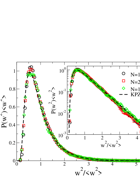
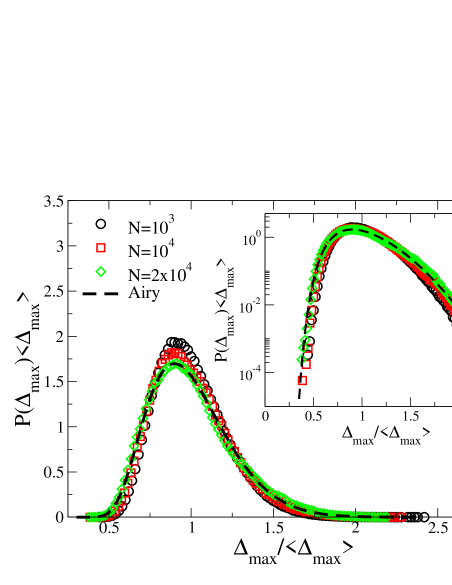
(a) Width distribution	(b) Maximum fluctuations distribution

Figure 1: (a) The scaled distribution of the width of task-completion landscapes on a one-dimensional regular network. The inset is the same graph in log-linear scale. The dashed curve is the scaled width distribution of KPZ/EW surface Foltin et al. (1994). (b) The scaled distribution of the maximum fluctuations in the same network. The inset is in log-linear scale and the dashed curve is the appropriately scaled Airy distribution function Majumdar and Comtet (2004, 2005).

The extreme-value limit theorems summarized in the previous section are valid only for independent (or short-range correlated) random variables. Since the “heights” (local progress) in task-completion landscapes of regular networks are strongly correlated, the known extreme-value limit theorems cannot be used. Some remarkable recent analytic work yielded the distribution of the extreme heights for the one-dimensional EW/KPZ steady-state surface Majumdar and Comtet (2004, 2005); Kearney and Majumdar (2005); Schehr and Majumdar (2006). Although the local microscopic rule for the evolution of the task-completion landscapes are different, they belong to the same EW/KPZ universality class in one dimension Barabási and Stanley (1995), and hence, expected to exhibit the same universal distribution for the extreme fluctuations. Equation (23) suggests that, similar to the width and its distribution, there is a single scale governing the diverging extremes fluctuations, and hence, the normalized probability density function of the maximum relative fluctuations $\Delta_{\max}$ has a universal scaling form, $P(\Delta_{\max})\sim N^{-\alpha}f(\Delta_{\max}/N^{\alpha})$. For the 1D EW/KPZ surface with periodic boundary conditions ($\alpha$$=$$1/2$), by using path integral techniques, Majumdar and Comtet Majumdar and Comtet (2004, 2005) found $f(x)$ to be the so-called Airy distribution function. Our simulation results show that the appropriately scaled maximum relative height distributions are in agreement with the theoretical distribution as can be seen in Fig. 1(b).

Recently, we have studied the extreme fluctuations in task-completion landscapes on SW networks Guclu and Korniss (2004, 2005). In particular, we considered two SW-synchronized network models: in one case a small (variable) density of random links were added on top of a one-dimensional ring; in the other case, each node had exactly one random (possibly long-range) connection, and the “coupling strength” (relative frequency of synchronization through the long-range link) was varied. The basic findings were the same for both cases. As a result of the non-zero density or non-zero strength of random links, the correlation length $\xi$ becomes finite in such networks (as opposed to the diverging correlation length on the one-dimensional ring.) This important property is intimately related to the emergence of an effective non-zero mass of the corresponding network propagator (the inverse of the network Laplacian) Kozma et al. (2004). This is the fundamental effect of extending the original dynamics to a SW network: it decouples the fluctuations of the originally correlated landscape. Then, the extreme-value limit theorems can be applied using the number of independent blocks $N/\xi$ in the system Bouchaud and Mézard (1997); Baldassarri (2000). For short tailed noise, the local individual task fluctuations also exhibit short (exponential-like) tails, $S(\Delta_{i})\simeq\exp[-c(\Delta_{i}/w)^{\delta}]$, where $\Delta_{i}$$=$$\tau_{i}$$-$$\bar{\tau}$ is the relative “height” measured from the mean at site $i$. (Note that the exponent $\delta$ for the tail of the local relative height distribution may differ from that of the noise as a result of the collective (possibly non-linear) dynamics, but the exponential-like feature does not change.) Then the (appropriately scaled) largest fluctuations are governed by the Gumbel pdf [Eq. (12)], and the average maximum relative height scales as

$$\langle\Delta_{\max}\rangle\simeq w\left(\frac{\ln(N/\xi)}{c}\right)^{1/\delta}\simeq\frac{w}{c^{1/\delta}}\left[\ln(N)\right]^{1/\delta}\;.$$ (24)

(Note, that both $w$ and $\xi$ approach their finite asymptotic $N$-independent values for SW-coupled systems, and the only $N$-dependent factor is $\ln(N)$ for large $N$ values.) In SW synchronized systems with unbounded local variables driven by exponential-like noise distribution (such as Gaussian), the extremal fluctuations increase only logarithmically with the number of nodes. This weak divergence, which one can regard as marginal, ensures synchronization for practical purposes in coupled multi-component systems.

Note that the exact “microscopic” dynamics [Eq. (17)] based on the task-completion rule, is inherently non-linear, but the effects of the non-linearities only give rise to a renormalized non-zero effective mass Korniss et al. (2003). Thus, the synchronization dynamics is effectively governed by EW relaxation in a SW, yielding a finite correlation length and, consequently, the slow logarithmic increase of the extreme fluctuations with the system size [Eq. (24)]. Also, for the task-completion landscapes, the local height distribution can be asymmetric with respect to the mean, but the average size of the height fluctuations is, of course, finite for both above and below the mean. This specific characteristic simply yields different prefactors for the extreme fluctuations [Eq. (24)] above and below the mean, leaving the logarithmic scaling with $N$ unchanged.

Simulating the exact local task-completion rule Eq. (17), we observed, that the local height fluctuations exhibit simple exponential tails, hence $\delta=1$ and the extremes scale as $\ln(N)$ with the number of nodes Guclu and Korniss (2004, 2005); Guclu et al. (2004). The largest relative deviations below the mean $\langle\Delta_{min}\rangle$, and the maximum spread $\langle\Delta_{max-min}\rangle$ follows the same logarithmic scaling with the system size $N$.

IV Scale-Free Task-Completion Networks

Recent studies show that many natural and artificial systems such as the Internet, World Wide Web, scientific collaboration networks, and e-mail networks have power-law degree (connectivity) distributions Boccaletti et al. (2006), i.e., the probability of having nodes with $k$ degrees is $P(k)\sim k^{-\gamma}$ where $\gamma$ is usually between $2$ and $3$. These systems are commonly known as power-law or scale-free networks since their degree distributions are free of scale and follow power-law distributions over many orders of magnitude. Scale-free networks have many interesting properties such as high tolerance to random errors and attacks (yet low tolerance to attacks targeted at hubs) Albert et al. (2000), high synchronizability Guclu (2005); Toroczkai et al. (2006); Korniss (2006), and resistance to congestion Toroczkai and Bassler (2004); Toroczkai et al. .

In this paper, in part, we employed the Barabási-Albert (BA) model of network growth inspired by the formation of World Wide Web Barabási and Albert (1999) to generate scale-free networks. This model is based on two basic observations: growth and preferential attachment. The basic idea is that the high-degree nodes attract links faster than low-degree nodes. The network starts growing from $m_{0}$$=$$m+1$ nodes and at every time step a new node with $m$ (“stubs”) possible links is added to the network. The probability that the new node $j$ is connected to already existing node $i$ is linearly proportional to the degree of the node $j$, i.e., ${\rm Pr}(i\rightarrow j)$$=$$k_{j}/\sum_{l}k_{l}$. Once the given number of nodes $N$ is reached in the network, the process is stopped. For the BA network, the degree distribution is a power law in the asymptotic system size limit ($N$$\rightarrow$$\infty$, also called thermodynamic limit), $P_{BA}(k)\simeq 2m^{2}/k^{3}$.(In obtaining this normalization, one replaces the sum by the integral over the degree.) Since every node has $m$ links initially, the network at time $t$ will have $N$$=$$m_{0}+t$ nodes and $E$$=$$mt$ links, thus the average degree $\langle k\rangle$$=$$2m$ for large enough $t$. The special case of the model when $m=1$ creates a network without any loops, i.e., the network becomes a tree with no clustering.

Another model we employed to generate scale-free networks and to compare with the BA model is the configuration model (CM). The CM Bender and Canfield (1978); Molloy and Reed (1995, 1998) was introduced as an algorithm to generate random networks with a given degree distribution. Although CM has been considered to generate uncorrelated random networks, it was shown that it has correlations, especially between the nodes with larger degrees Catanzaro et al. (2005); Boguná et al. (2004). In CM, the vertices of the graph are assigned a sequence of degrees $\{k_{i}\}_{i=0}^{N},m\leq k_{i}\leq k_{c}$ from a desired distribution $P(k)$. (There is an additional constraint that the $\sum_{i}k_{i}$ must be even.) Then, pairs of nodes are chosen randomly and connected by undirected edges. This model generates a network with the expected degree distribution and no degree correlations; however, it allows self-loops and multiple-connections when it is used as described above. It was proven in Ref. Boguná et al. (2004) that the number of multiple connections when the maximum degree is fixed to the system size, i.e., $k_{c}$$=$$N$, scales with the system size $N$ as $N^{3-\gamma}\ln N$. After this procedure we simply delete the multiple connections and self-loops from the network which gives a very marginal error in the degree distribution exponent. This might also cause that some negligible number of nodes in the network to have degrees less than the fixed minimum degree ($m$) value or even zero. One another characteristic of the CM is that the network may not be a connected network for small values of $m$ such as $1$ and even $2$, i.e., it has disconnected clusters (or components). For high values of $m$, the network is almost surely connected having one giant component including all the nodes. The degree distribution of SF networks with degree exponent $\gamma$ (for $k_{c}\gg m$) can be written as

$$P(k)\simeq(\gamma-1)m^{\gamma-1}k^{-\gamma}\;,$$ (25)

where $m$ is the minimum degree in the network, and again, in obtaining the above normalization, we replaced the sum by the integral over the degree. Then the average and the minimum degree are then related through $\langle k\rangle=m(\gamma-1)/(\gamma-2)$.

IV.1 Mean-Field and Exact Numerical Diagonalization Approaches for the EW Process on SF Networks

We, again, can gain some insight to the problem by first considering the linearized effective equations of motion, i.e., the EW process [Eq. (18)] on a SF network. In the mean-field (MF) approximation, local task fluctuations about the mean are decoupled and reach a stationary distribution with variance Korniss (2006)

$$\left\langle(\tau_{i}-\bar{\tau})^{2}\right\rangle\approx 1/C_{i}\;.$$ (26)

For identical (unweighted) couplings (with unit link strength without loss of generality), $C_{ij}$ is simply the adjacency matrix, hence, $C_{i}=\sum_{l}C_{il}=k_{i}$, i.e., the degree of node $i$. Then, for the width, one can write

$$\langle w^{2}\rangle=\frac{1}{N}\sum_{i=1}^{N}\left\langle(\tau_{i}-\bar{\tau})^{2}\right\rangle\approx\frac{1}{N}\sum_{i}\frac{1}{C_{i}}=\frac{1}{N}\sum_{i}\frac{1}{k_{i}}\approx\int_{m}^{\infty}dk\frac{P(k)}{k}\;,$$ (27)

where using infinity as the upper limit in the above integral is justified for SF networks as $N\to\infty$, since $\gamma>0$. Using the degree distribution of SF networks given by Eq. (25), one finally obtains the mean-field expression for the width

$$\langle w^{2}\rangle\approx\frac{1}{m}\frac{(\gamma-1)}{\gamma}=\frac{1}{\langle k\rangle}\frac{(\gamma-1)^{2}}{\gamma(\gamma-2)}\;.$$ (28)

The main message of the above result is that the width approaches a finite value in the limit of $N\to\infty$, and for the linearized problem, should scale as $\langle w^{2}\rangle\sim 1/m\sim 1/\langle k\rangle$.

Extracting the steady-state width from exact numerical diagonalization Korniss et al. (2006); Korniss (2006) through

$$\langle w^{2}\rangle=\frac{1}{N}\sum_{k=1}^{N-1}\frac{1}{\lambda_{k}}\;,$$ (29)

where $\lambda_{k}$ are the non-zero eigenvalues of the network Laplacian on the corresponding SF network, supports these MF predictions [Fig. 2]. Except for the $m=1$ BA network (when the network is a scale-free tree), finite-size effects are negligible as the width approaches a finite value in the $N\to\infty$ limit [Fig. 2(a)]. For $m=1$, the width weakly (logarithmically) diverges with the system size [Fig. 2(a) inset]. A closer look at the spectrum reveals that the gap approaches a non-zero value for $m>1$ as $N\to\infty$, while it slowly vanishes for the $m=1$ BA network. As can be expected, Fig. 2(b) (inset) indicates that MF scaling Eq. (28) for the width works well for sufficiently large minimum (and average) degree, $m\stackrel{{\scriptstyle>}}{{\sim}}{\cal O}(10)$. Figure  2(c) also shows results for the CM network for two values of $\gamma$, and the corresponding MF result.

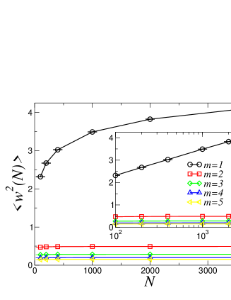
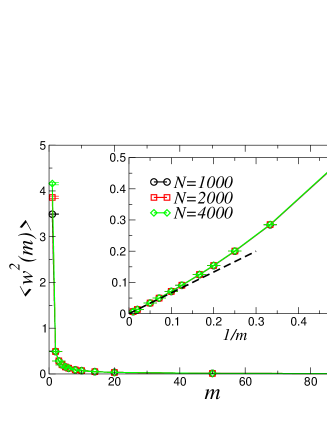
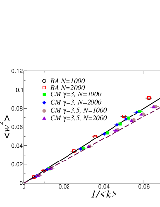
(a) Width vs system size	(b) Width vs m	(c) Width vs $1/\langle k\rangle$

Figure 2: Steady-state width of the EW synchronization landscape from exact numerical diagonalization using Eq. (29). (a) For the BA network, as a function of $N$ for various values of the minimum degree $m$. The inset shows the same data on log-lin scales. (b) For the BA network, as a function of $m$ for different system sizes $N$. The inset shows the behavior of the width vs $1/m$; the solid straight line represents the MF result Eq. (28). (c) For the BA and CM networks (with $\gamma=3.0$ and $\gamma=3.5$) as a function of $1/\langle k\rangle$, where $\langle k\rangle$ is the average degree, for two system sizes. The bold straight solid and dashed lines correspond to the MF result Eq. (28) with $\gamma=3.0$ and $\gamma=3.5$, respectively.

We also note that the average width, in principle, can also be obtained by employing the density of states (dos) $\rho(\lambda)$ of the underlying network Laplacian through $\langle w^{2}\rangle=(1/N)\sum_{l=1}^{N-1}1/\lambda_{l}\simeq\int(1/\lambda)\rho(\lambda)d\lambda$, in the asymptotic large-$N$ limit Kozma et al. (2004); Kozma and Korniss (2004). Obtaining the dos analytically, however, is a rather challenging task. Just recently, using the replica method Bray and Rodgers (1988); Rodgers et al. (2005), Kim and Kahng obtained the dos for the Laplacian of SF graphs Kim and Kahng , which they were able to evaluate in the asymptotic $1$$<<$$\langle k\rangle$$<<$$N$ limit. Utilizing their result, we have checked and found full agreement with Eq. (28) for the width.

While our MF approach above does not directly address the typical size of the maximum relative height of the task-completion landscape, the finding that the width is finite in the $N\to\infty$ limit suggests that correlations between height fluctuations at different nodes are weak (with the exception of the $m=1$ BA tree). Then, one can argue on the scaling of the extremes as follows. The largest fluctuations will most likely emerge from the nodes with (or close to) the smallest degree $m$ [Eq. (26)]. The typical size of the fluctuations on such nodes, according Eq. (26), is $\sqrt{\langle(\tau_{i}-\bar{\tau})^{2}\rangle}_{k_{i}=m}\sim m^{-1/2}$. The expected number of nodes with the smallest degree $m$ is $N_{m}\sim NP(m)\sim(\gamma-1)(N/m)$. Thus, assuming that the fluctuations on these nodes are independent, we expect

$$\langle\Delta_{\max}\rangle=\langle\tau_{\max}-\bar{\tau}\rangle\sim\sqrt{\langle(\tau_{i}-\bar{\tau})^{2}\rangle}_{k_{i}=m}\left[\ln[(\gamma-1)(N/m)]\right]^{1/\delta}\sim m^{-1/2}\left[\ln(N)\right]^{1/\delta}\;,$$ (30)

and the distribution of the extremes is governed by the Gumbel distribution in the asymptotic large-$N$ limit. Note that the exponent $\delta$ depends on the details of the noise (or local stochastic task increments), e.g., $\delta$$=$$2$ for Gaussian-like tails and $\delta$$=$$1$ for exponential tails. The $m^{-1/2}$ pre-factor is also specific to the linear EW coupling on the network by virtue of Eq. (26), and we do not expect to be generally applicable. We do expect, however, that the weak logarithmic divergence with the system size, Eq. (30), governed by the Gumbel distribution, will hold for the actual simulated task-completion landscape which evolves according to the synchronization rule Eq. (17), on SF networks.

IV.2 Simulation Results

In this subsection we present detailed results and analysis of the simulations of the exact task-completion rule Eq. (17) on BA and CM networks. We simulated the task-completion system on these networks and measured the steady-state width Eq. (21) and maximum fluctuations over many different network realizations and generated their distributions.

Fig. 3 shows the average maximum fluctuations and the width as function of $m$ for different system sizes ranging from 100 to 10,000. Each data point was obtained by averaging over ten different network realizations. As it can be seen from Fig. 3(a), $\langle\Delta_{\max}\rangle$ rapidly approaches a system-size-dependent constant. For the $m=1$ BA model, the network is a tree, and $\langle\Delta_{\max}\rangle$ is visibly larger than for higher values of $m$. Figure 3(b) contains the same data points as Fig. 3(a), but the data is plotted as function of the system size, for different values of $m$. The average maximum fluctuations in Fig. 3(b) scale logarithmically (or diverge weakly) with the system size for all values of $m$. Again, the $m=1$ case is different from others in terms of the pre-factors, although they all exhibit logarithmic divergence. Thus, for BA networks, we find

$$\langle\Delta_{\max}\rangle\sim\ln(N)\;.$$ (31)

supporting the MF prediction Eq. (30). The “clean” logarithmic scaling in Fig. 3(b) is the result of the individual task distributions $P(\tau_{i}-\bar{\tau})$ having an exponential tail ($\delta=1$) for the task-completion rule.

With the exception of the $m$$=$$1$ BA tree, the width converges to an essentially system-size-independent, but non-zero, value [Fig. 3(c)]. The main difference, with respect to the MF prediction, is the non-vanishing “intrinsic” width as $m\to\infty$. This behavior is due to the specific synchronization rule Eq. (17). Namely, when $m$ is large, only a couple of nodes are allowed to increment, hence the landscape fluctuations are essentially governed by the stochastic task increments at these nodes. Since the variance of the local fluctuations is unity, the width of the landscape converges to unity for large $m$ [Fig. 3(c)]. It can be seen in Fig. 3(d) that the width has a logarithmic divergence for $m=1$ and it is a constant for $m>1$, i.e., for large $N$

$$\langle w^{2}(N)\rangle\sim\left\{\begin{array}[]{ll}\ln(N),&\text{if}~{}m=1\\ \text{const.},&\text{if}~{}m>1\\ \end{array}\right.\;.$$ (32)

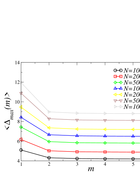
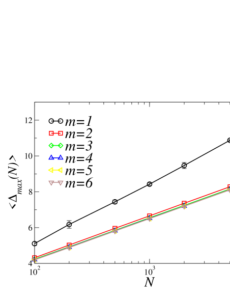
(a) Maximum fluctuations vs m	(b) Maximum fluctuations vs system size
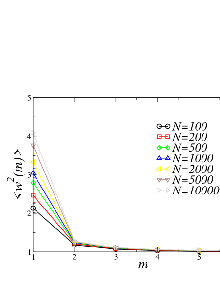
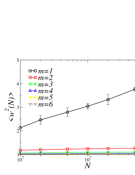
(c) Width vs m	(d) Width vs system size

Figure 3: Average maximum fluctuations and average width for SF networks generated by the BA model. The data points are obtained by averaging over ten different network realizations.

The CM network has very similar characteristics to the BA model in terms of the scaling of maximum fluctuations and width. Fig. 4(a) shows that the average maximum fluctuations for CM network with $\gamma=3$, as a function of $m$, have the same behavior as for the BA model. Since the CM generates a (single-component) connected network with very low probability for $m=1$, we only present results for $m>1$. As it can be seen in Fig. 4(b), $\langle\Delta_{\max}\rangle$ increases logarithmically with the system size. The data points were obtained by averaging over ten different realizations of the network. One observes that at low values of $\gamma$, $\langle\Delta_{\max}(m=2)\rangle$ is closer to $\langle\Delta_{\max}(m>2)\rangle$ and the difference increases as $\gamma$ increases. This implies that having fewer high-degree nodes in the network ($\gamma=4$) separates $\langle\Delta_{\max}(m=2)\rangle$ from $\langle\Delta_{\max}(m>2)\rangle$.

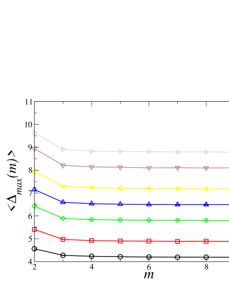
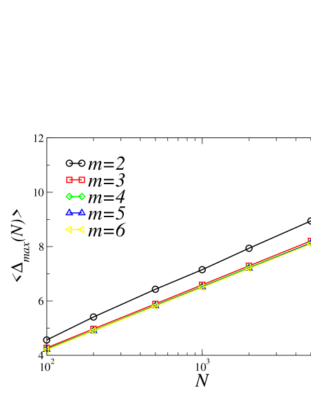
(a) Maximum fluctuations vs $m$	(b) Maximum fluctuations vs system size
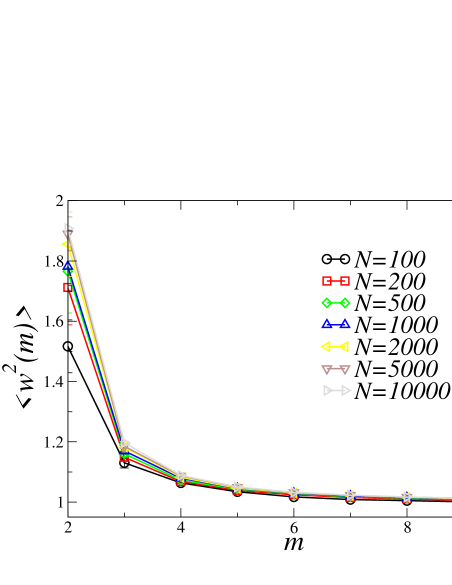
(c) Width vs m	(d) Width vs system size

Figure 4: Average maximum fluctuations and the width for SF CM networks with $\gamma=3$ versus system size and $m$. The data points are obtained by averaging over ten different network realizations.

The average width as a function of $m$ [Fig. 4(c)] for $\gamma=3$ decays and reaches its asymptotic value. The scaling of the width as a function of the system size is in Fig. 4(d). The error bars are quite visible although we use at least ten different network realizations. There is a slight increase in the width as a function of the system size for $m=2$, whereas for larger $m$, the width quickly saturates as a function of $N$.

Fig. 5(a) shows the individual task distributions (parent distributions for the extremes) for the BA network with $m=2$ and $N=10^{4}$. These distributions exhibit simple exponential tails ($\delta=1$) (inherited from the local exponential task-increments). The nodes for which the distributions presented in Fig. 5(a) were selected manually according to their degrees. We selected high (also maximum), middle and low (also minimum) degree nodes. The legend shows both the index of the node, which is the “age” of the node according to the preferential attachment procedure in the BA model, and its degree. For larger $m$ the distributions yield better collapse to an exponential, and also their negative parts (for the fluctuations below the mean) become smaller, i.e., the fluctuations are asymmetric about the mean (due to the specific local task-increment rules). It can also be seen that the negative part of the individual task distributions are not pure exponentials, i.e., $\delta>1$, which makes the convergence of the fluctuations of the minima ($\Delta_{min}$) toward their limiting Gumbel distribution much slower.

Figs. 5(b) and 5(c) show the distributions of the maximum fluctuations and the width for the BA model with $m=2$ and their comparison to the Gumbel and Gaussian distributions, respectively. The insets in Figs. 5(b) and 5(c) have the same data as the main graph but scaled to zero mean and unit variance, and in a log-linear scale to show the collapse to the limit distributions in the tails. The pure exponential behavior of individual task distributions in Fig. 5(a) suggests that the limit distribution for the maximum fluctuations would be a Gumbel distribution. As it can be seen in Fig. 5(b) the limit distributions have better collapse as the system size gets larger. The width distributions for the BA model with $m=2$ are plotted in Fig. 5(c). The mean-field approximation predicts that the local task fluctuations are decoupled and consequently the distribution of the width converges to a Gaussian for large enough systems. We verified this prediction and showed that the width distributions converge to delta functions, and when they are scaled to zero mean and unit variance they collapse to a standard Gaussian distribution for large enough system size. When $m=1$ the width distribution converges to a nontrivial shape with an exponential tail.

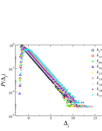
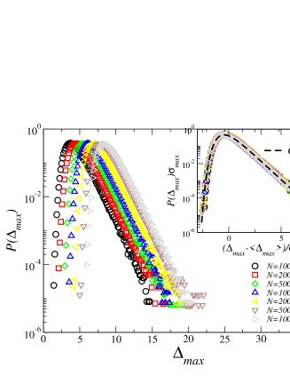
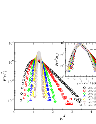
(a) Individual fluctuations distribution	(b) Maximum fluctuations distribution	(c) Width distribution

Figure 5: Distribution of individual fluctuations (a), maximum fluctuations (b) and the width (c) for the BA model with $m=2$. The different individual fluctuations distributions in (a) are for different degree values ranging from the maximum to the minimum. The inset in (b) shows the maximum fluctuations distribution scaled to zero mean and unit variance in a log-linear scale. The dashed curves in the insets represent the Gumbel pdf [Eq. (16)] in (b) and Gaussian pdf in (c) scaled in the same way. The system size is $N=10^{4}$.

Similar to individual task distributions in the BA model, the CM has pure exponential distributions in the tail as shown in Fig. 6(a) for $m=3$, $\gamma=3$, and system size $N=10^{4}$. The nodes are selected according to their degrees, i.e., a few high, middle and low-degree nodes. The maximum fluctuation distributions converge to Gumbel distributions even for small systems as it can be seen in Fig. 6(b). It can be concluded for the CM that the width distributions converge to delta functions as system size goes to infinity and when they are scaled to zero mean and unit variance they converge to the standard Gaussian [Fig. 6(c)]. For the somewhat subtle case of the CM network with $m=2$ the convergence to a finite width is slow [see Fig. 4(d)] possibly due to strong finite system-size effects.

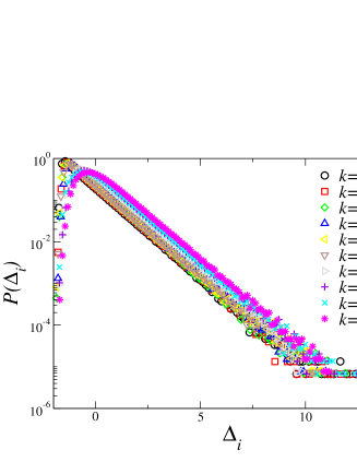
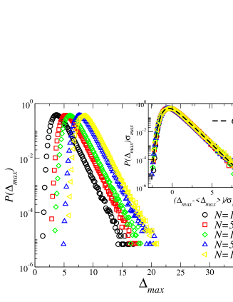
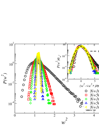
(a) Individual fluctuations distribution	(b) Maximum fluctuations distribution	(c) Width distribution

Figure 6: Same as Fig. 5 for the CM network with $\gamma=3$ and $m=3$.

V Summary and Conclusions

In summary, we considered the average and maximum fluctuations above the mean in scale-free task-completion landscapes with local relaxation, unbounded local variables, and short-tailed noise. We argued, that when the interaction topology is scale-free, having a power-law degree distribution, the statistics of the extremes is governed by the Gumbel distribution while the distribution of average fluctuations converges to a Gaussian when appropriately scaled. This finding directly addresses synchronizability in generic task-completion systems with scale-free network topology where relaxation through the links is the relevant node-to-node process and effectively governs the dynamics. Analogous questions for heavy-tailed noise distribution on complex networks have relevance to various transport phenomena in natural, artificial, and social systems de Menezes and Barabási (2004); Barabási et al. (2004); Crovella and Bestavros (1997); Crovella et al. (1998); Leland et al. (1994); Csabai (1994); Paxson and Floyd (1995). For example, “bursty” temporal processes in queuing networks have been recently attributed to online activities initiated by humans Barabási (2005). Correspondingly, one shall then study extreme fluctuations in task-completion landscapes where the local task increments are power-law distributed. Heavy-tailed noise typically generates similarly tailed local field variables through the collective dynamics in SW Guclu et al. (2004); Guclu and Korniss (2005) and SF networks Guclu et al. . Then, the largest fluctuations will likely diverge as a power law with the system size, expectedly governed by the Fréchet distribution Gumbel (1958); Galambos (1987).