Single-site Anderson model. II Perturbation theory of symmetric model

Abstract

The strong electron correlations caused by Coulomb interaction of impurity electrons are taken into account. The infinite series of diagrams containing irreducible Green’s functions are summed. For symmetric Anderson model we establish the antisymmetry property of the impurity Green’s function, formulate the exact Dyson type equation for it, find the approximate correlation function $Z_{\sigma}(i\omega$) and solve the integral equation which determines the full propagator of the impurity electrons. Analytical continuation of the obtained Matsubara Green’s function determines the retarded one and gives the possibility to find the spectral function of impurity electrons. The existence of two resonances of this function has been proved. The smooth behaviour was found near the Fermi surface. The two resonances situated symmetrical to the Fermi surface correspond to the energies of quantum transitions of the impurity electrons. The widths and heights of these resonances are established.

I Introduction

We shall investigate the properties of the normal state of single-site Anderson model. For that we shall use the results of diagrammatic theory for this model developed in our previous paper^[1]. In that investigation the notion of irreducible Green’s function has been introduced. These functions contain the main spin, charge and pairing fluctuations caused by the strong Coulomb repulsion of impurity electrons. We have determined the notion of correlation function $Z_{\sigma\sigma^{\prime}}$ as composed from strong connected diagrams containing the irreducible Green’s functions. In superconducting state of the system there are additional correlation functions $Y_{\sigma\sigma^{\prime}}$ and $\overline{Y}_{\overline{\sigma}\sigma^{\prime}}$ which are the order parameters of the system. The correlation functions are the main elements of the Dyson type equations for one–particle renormalized Green’s function of conducting and impurity electrons. We shall restrict ourselves only by the discussion of the properties of the normal phase of the system and determine the corresponding Green’s functions of conduction and impurity electrons:

$$G_{\sigma\sigma^{\prime}}(\mathbf{k,}\tau|\mathbf{k}^{\prime},\tau^{\prime}) = -\left\langle TC_{\mathbf{k}\sigma}(\tau)\overline{C}_{\mathbf{k}^{\prime}\sigma^{\prime}}(\tau^{\prime})U(\beta)\right\rangle_{0}^{c},$$

$$g_{\sigma\sigma^{\prime}}(\tau|\tau^{\prime}) = -\left\langle Tf_{\sigma}(\tau)\overline{f}_{\sigma^{\prime}}(\tau^{\prime})U(\beta)\right\rangle_{0}^{c},$$

where index ”$c$” means connected.

Fourier representation is denoted as $G_{\sigma\sigma^{\prime}}(\mathbf{k},\mathbf{k}^{\prime}|i\omega)$ and $g_{\sigma\sigma^{\prime}}(i\omega)$ correspondingly. For these two functions we have obtained the results^[1] :

$$G_{\sigma}(\mathbf{k},\mathbf{k}^{\prime}|i\omega) = \delta_{\mathbf{kk}^{\prime}}G_{\sigma}^{0}(\mathbf{k}|i\omega)+\frac{V_{\mathbf{k}}V_{\mathbf{k}^{\prime}}^{\ast}}{N}G_{\sigma}^{0}(\mathbf{k}|i\omega)g_{\sigma}(i\omega)G_{\sigma}^{0}(\mathbf{k}^{\prime}|i\omega),$$

$$g_{\sigma}(i\omega) = \frac{\Lambda_{\sigma}(i\omega)}{1-\Lambda_{\sigma}(i\omega)G_{\sigma}^{0}(i\omega)},$$ (2)

$$\Lambda_{\sigma}(i\omega) = g_{\sigma}^{0}(i\omega)+Z_{\sigma}(i\omega),$$

where zero order propagators of the conduction and impurity electrons have the form ($\overline{\sigma}=-\sigma$).

$$G_{\sigma}^{0}(\mathbf{k}|i\omega) = (i\omega-\epsilon(\mathbf{k}))^{-1},$$

$$g_{\sigma}^{0}(i\omega) = \frac{1-n_{\overline{\sigma}}}{i\omega-\epsilon_{f}}+\frac{n_{\overline{\sigma}}}{i\omega-\epsilon_{f}-U},$$

$$n_{\overline{\sigma}} = \frac{\exp(-\beta\epsilon_{f})+\exp\left[-\beta(2\epsilon_{f}+U\right]}{Z_{0}},$$ (3)

$$Z_{0} = 1+2\exp(-\beta\epsilon_{f})+\exp\left[-\beta(2\epsilon_{f}+U\right],$$

$$G_{\sigma}^{0}(i\omega) = \frac{1}{N}\sum\limits_{\mathbf{k}}|V_{\mathbf{k}}|^{2}G_{\sigma}^{0}(\mathbf{k}|i\omega)=\int\frac{V^{2}(\epsilon)\rho_{0}(\epsilon)d\epsilon}{i\omega-\epsilon}.$$

Here $\epsilon(\mathbf{k})$ is the energy of conduction band and $\epsilon_{f}$ of local impurity electrons, $\rho_{0}(\epsilon)$ is the density of states of the bare conduction band and matrix element of hybridization $V_{\mathbf{k}}$ is supposed dependent of the energy. $U$ is Coulomb repulsion of the impurity electrons. $\omega\equiv\omega_{n}=(2n+1)\pi/\beta$ is odd Matsubara frequency. The equations (2) are exact, but for correlation function $Z_{\sigma}(i\omega)$ doesn’t exist exact Dyson type equation and only the approximate contribution can be available: see $Fig$. 9 of paper^[1]. Our main approximation formulated in paper^[1] comes to the summation of the ladder diagrams which will be enough to obtain the main contributions of the spin and charge fluctuations. This approximation has used only the simplest irreducible Green’s function $g_{2}^{(0)ir}$ which is iterated many times. It has the form:

$$Z_{\sigma\sigma^{\prime}}(\tau-\tau^{{}^{\prime}}) = -\sum\limits_{\mathbf{k}_{1}\mathbf{k}_{2}\sigma_{1}\sigma_{2}}\int\limits_{0}^{\beta}d\tau_{1}\int\limits_{0}^{\beta}d\tau_{2}g_{2}^{(0)ir}[\sigma,\tau;\sigma_{1},\tau_{1}|\sigma_{2},\tau_{2};\sigma^{\prime},\tau^{\prime}]\frac{1}{N}V_{\mathbf{k}_{1}}^{\ast}V_{\mathbf{k}_{2}}G_{\sigma_{2}\sigma_{1}}(\mathbf{k}_{2},\tau_{2}|\mathbf{k}_{1},\tau_{1}),$$ (4)

or in Fourier representation

$$Z_{\sigma\sigma^{\prime}}(i\omega) = -\frac{1}{\beta}\sum\limits_{\omega_{1}}\sum\limits_{\sigma_{1}\sigma_{2}}\sum\limits_{\mathbf{k}_{1}\mathbf{k}_{2}}\widetilde{g}_{2}^{(0)ir}[\sigma,i\omega;\sigma_{1},i\omega_{1}|\sigma_{2},i\omega_{1};\sigma^{\prime},i\omega]\frac{1}{N}V_{\mathbf{k}_{1}}^{\ast}V_{\mathbf{k}_{2}}G_{\sigma_{2}\sigma_{1}}(\mathbf{k}_{1},\mathbf{k}_{2}|i\omega_{1}).$$ (5)

Here we take into account the conservation law of the frequencies:

$$g_{2}^{(0)ir}[\sigma,i\omega;\sigma_{1},i\omega_{1}|\sigma_{1},i\omega_{1};\sigma^{\prime},i\omega^{\prime}] = \beta\delta(\omega-\omega^{\prime})\widetilde{g}_{2}^{(0)ir}[\sigma,i\omega;\sigma_{1},i\omega_{1}|\sigma_{2},i\omega_{1};\sigma^{\prime},i\omega].$$ (6)

In paramagnetic phase we have more simple equation ($\sigma^{\prime}=\sigma$):

$$Z_{\sigma}(i\omega) = -\frac{1}{\beta}\sum\limits_{\omega_{1}}\sum\limits_{\sigma_{1}}\widetilde{g}_{2}^{(0)ir}[\sigma,i\omega;\sigma_{1},i\omega_{1}|\sigma_{1},i\omega_{1};\sigma,i\omega]G_{\sigma_{1}}(i\omega_{1}),$$ (7)

where

$$G_{\sigma}(i\omega)=\frac{1}{N}\sum\limits_{\mathbf{k}_{1}\mathbf{k}_{2}}V_{\mathbf{k}_{1}}^{\ast}V_{\mathbf{k}_{2}}G_{\sigma}(\mathbf{k}_{1},\mathbf{k}_{2}|i\omega).$$ (8)

On the base of equations (2) and (3) the last function (8) can be presented in the form:

$$G_{\sigma}(i\omega)=G_{\sigma}^{0}(i\omega)+[G_{\sigma}^{0}(i\omega)]^{2}g_{\sigma}(i\omega)=\frac{G_{\sigma}^{0}(i\omega)}{1-\Lambda_{\sigma}(i\omega)G_{\sigma}^{0}(i\omega)}.$$ (9)

By using the definition (2) of correlation function of normal state $\Lambda_{\sigma}(i\omega)$ and approximation (7) for function $Z_{\sigma}(i\omega)$, we obtain the final integral equation for $\Lambda_{\sigma}$:

$$\Lambda_{\sigma}(i\omega)=g_{\sigma}^{(0)}(i\omega)-\frac{1}{\beta}\sum\limits_{\omega_{1}}\sum\limits_{\sigma_{1}}\widetilde{g}_{2}^{(0)ir}[\sigma,i\omega;\sigma_{1},i\omega_{1}|\sigma_{1,}i\omega_{1};\sigma,i\omega]\frac{G_{\sigma_{1}}^{0}(i\omega_{1})}{1-\Lambda_{\sigma_{1}}(i\omega_{1})G_{\sigma_{1}}^{0}(i\omega_{1})}.$$ (10)

In the second Section of this paper we shall discuss the simplest case of symmetric impurity Anderson model with the condition $2\epsilon_{f}+U=0$. In Section III the spectral function of the impurity electrons is analyzed and the last Section IV contains the conclusions.

II Symmetric model

In symmetric case when $\epsilon_{f}=-U/2<0$ and $\epsilon_{f}+U=U/2>0$ we have more simple equations:

$$g_{\sigma}^{0}(i\omega) = \frac{i\omega}{(i\omega)^{2}-(U/2)^{2}},$$

$$Z_{0} = 2(1+\exp(-\beta\epsilon_{f}))=2(1+\exp(\beta U/2)),$$

$$n_{\sigma} = 1/2$$ (11)

and the antisymmetry property of zero order impurity Green’s function $g_{\sigma}^{0}(-i\omega)=-g_{\sigma}^{0}(i\omega)$ takes place.

Additionally we suppose also the evenness of the matrix element $V(\epsilon)$ and of the bare density of state $\rho_{0}(\epsilon)$. In this case the function $G_{\sigma}^{0}(i\omega)$ is also antisymmetric $G_{\sigma}^{0}(-i\omega)=-G_{\sigma}^{0}(i\omega)$.
Thanks these antisymmetry properties we shall look for the antisymmetric solution

$$\Lambda_{\sigma}(-i\omega)=-\Lambda_{\sigma}(i\omega)$$ (12)

of the equation (10). Analytical continuation of these functions have the property of oddness of their real parts and evenness of imaginary parts in conformity with equations

$$g_{\sigma}^{0}(E+i\delta) = -g_{\sigma}^{0}(-E-i\delta),$$

$$G_{\sigma}^{0}(E+i\delta) = -G_{\sigma}^{0}(-E-i\delta),$$ (13)

$$\Lambda_{\sigma}^{0}(E+i\delta) = -\Lambda_{\sigma}^{0}(-E-i\delta),$$

where

$$G_{\sigma}^{0}(E+i\delta) = I(E)-i\Gamma(E),$$

$$I(E) = P\int\frac{|V(\epsilon)|^{2}\rho_{0}(\epsilon)d\epsilon}{E-\epsilon},$$ (14)

$$\Gamma(E) = \pi|V(E)|^{2}\rho_{0}(E).$$

$I(E)$ is the principal part of the integral. This function is antisymmetric. $\Gamma(E)$ is the band width of the virtual level and an even function of energy. The symmetric impurity Anderson model has the advantage to be of a simple form for the irreducible two particles Green’s functions in different spin and frequency channels. In this special case we have^[2,3]

$$\widetilde{g}_{2}^{(0)ir}[\sigma,i\omega;\sigma,i\omega_{1}|\sigma,i\omega_{1};\sigma,i\omega] = \frac{\beta(U/2)^{2}(1-\delta\omega\omega_{1})}{[(i\omega)^{2}-(U/2)^{2}][(i\omega_{1})^{2}-(U/2)^{2}]},$$ (15)

$$\widetilde{g}_{2}^{(0)ir}[\sigma,i\omega;\overline{\sigma},i\omega_{1}|\overline{\sigma},i\omega_{1};\sigma,i\omega]=\frac{U}{2}\left\{\frac{\beta U}{2}\frac{(1-\exp(\beta U/2))}{(1+\exp(\beta U/2))[\omega^{2}+(U/2)^{2}][\omega_{1}^{2}+(U/2)^{2}]}-\right.$$

$$-\frac{\beta U\delta(\omega-\omega_{1})\exp(\beta U/2)}{(1+\exp(\beta U/2))[\omega^{2}+(U/2)^{2}][\omega_{1}^{2}+(U/2)^{2}]}+\frac{\beta U\delta(\omega+\omega_{1})}{(1+\exp(\beta U/2))[\omega^{2}+(U/2)^{2}][\omega_{1}^{2}+(U/2)^{2}]}-$$

$$-\frac{2}{[\omega^{2}+(U/2)^{2}][\omega_{1}^{2}+(U/2)^{2}]}+4(U/2)^{2}\left[\frac{1}{[\omega^{2}+(U/2)^{2}][\omega_{1}^{2}+(U/2)^{2}]^{2}}+\right.$$ (16)

$$\left.\left.+\frac{1}{[\omega^{2}+(U/2)^{2}]^{2}[\omega_{1}^{2}+(U/2)^{2}]}\right]\right\}.$$

Now we come back to equation (10) and note that thanks the antisymmetry property (12) of $\Lambda_{\sigma}(i\omega)$ function only those terms of equations (15) and (16) which contain Kronecker $\delta$ - symbols give the non zero contribution in the right hand part of it. The result of summation has the form:

$$\Lambda_{\sigma}(i\omega)=\frac{i\omega}{(i\omega)^{2}-(U/2)^{2}}+\frac{3(U/2)^{2}}{[(i\omega)^{2}-(U/2)^{2}]^{2}}\frac{G_{\sigma}^{0}(i\omega)}{[1-\Lambda_{\sigma}(i\omega)G_{\sigma}^{0}(i\omega)]}.$$ (17)

We notice that the scattering channel with opposite spins (16) gives in equation (17) the twice contribution in comparison with parallel spin channel (15) and both of them are added together giving the factor 3 in the right - hand part of equation (17). There are two solutions of equation (17) and we take that of them which has the correct asymptotic behavior $\lambda_{\sigma}(i\omega)\rightarrow\frac{1}{i\omega}$ when $|\omega|$ tends to infinity. This solution has the form:

$$\Lambda_{\sigma}(i\omega) = \frac{1}{2G_{\sigma}^{0}(i\omega)[(i\omega)^{2}-(U/2)^{2}]}\left\{[(i\omega)^{2}-(U/2)^{2}+i\omega G_{\sigma}^{0}(i\omega)]-[(i\omega)^{2}-(U/2)^{2}-\right.$$ (18)

$$- \left.i\omega G_{\sigma}^{0}(i\omega)]\sqrt{1-12Q(i\omega)}\right\}.$$

where

$$Q(i\omega)=\left(\frac{(U/2)G_{\sigma}^{0}(i\omega)}{(i\omega)^{2}-(U/2)^{2}-i\omega G_{\sigma}^{0}(i\omega)}\right)^{2}.$$ (19)

We have used that branch of square root which gives one when $Q(i\omega)$ tends to zero. On the base of equations (2) and (8) we obtain the renormalized impurity electron propagator

$$g(i\omega) = \frac{2[g^{0}(i\omega)[G^{0}(i\omega)]^{-1}+3Q(i\omega)(g^{0}(i\omega)-[G^{0}(i\omega)]^{-1})^{2}]}{[[G^{0}(i\omega)]^{-1}-g^{0}(i\omega)][1+\sqrt{1-12Q(i\omega)}+6Q(i\omega)(g^{0}(i\omega)G^{0}(i\omega)-1)]}.$$ (20)

In the last equations the spin index $\sigma$ is omitted because it is not significant. Equation (20) has been obtained by taking into account the spin and charge fluctuations contained in the correlation function $Z_{\sigma}(i\omega)$.

The spectral function of the impurity electrons is equal to

$$A_{f}\left(E\right)=-2Img\left({E+i\delta}\right),$$ (21)

where $g(E+i\delta)$ with $\delta=+0$ is the analytical continuation of the Matsubara to retarded Green’s function. In absence of the correlation function $Z_{\sigma}(i\omega)$ instead of equation (20) a more simple form appears

$$g_{\sigma}^{I}(i\omega)=\frac{g_{\sigma}^{0}(i\omega)}{1-g_{\sigma}^{0}(i\omega)G_{\sigma}^{0}(i\omega)}=\frac{1}{\left[g_{\sigma}^{0}(i\omega)\right]^{-1}-G_{\sigma}^{0}(i\omega)},$$ (22)

which can be named as Hubbard I approximation. This equation contains the zero order Green’s function $g^{0}(i\omega)$ determined by equation (11) and averaged by hybridization conduction electron function $G_{\sigma}^{0}(i\omega)$ of equation (14).

Analytical continuation of equation (22) gives

$$g_{\sigma}^{I}(E+i\delta)=\frac{1}{E-(U/2)^{2}E^{-1}-I(E)+i\Gamma(E)}.$$ (23)

We shall compare our renormalized spectral function (21) with more simple bare quantity $A_{f}^{0}(E)$:

$$A_{f}^{0}(E)=-2Img^{0}(E+i\delta) = 2\pi\delta(E-(U/2)^{2}E^{-1})=\pi\left(\delta(E-\frac{U}{2})+\delta(E+\frac{U}{2})\right)$$ (24)

and the value $A_{f}^{I}(E)$ obtained in Hubbard I approximation:

$$A_{f}^{I}(E) = -2Img^{I}(E+i\delta)=\frac{2\Gamma(E)}{\left(E-(U/2)^{2}E^{-1}-I(E)\right)^{2}+\Gamma^{2}(E)}.$$ (25)

Here the odd $I(E)$ and even $\Gamma(E)$ functions are determined by equation (14). Two resonances of equation (24) situated at energies $E=\pm\frac{U}{2}$ have not the width. After some interactions taken into account by Hubbard I approximation a new spectral function (25) appears. It has two resonances with shifted values of energies $E=\pm E_{0}$ determined by the presence of function $I(E)$:

$$E_{0}-\frac{(U/2)^{2}}{E_{0}}-I(E_{0})=0.$$ (26)

These resonances are broadened by the presence of the function $\Gamma(E)$, which is the width of the virtual level. This function $\Gamma(E)$ determines the height and width of the both resonances. Near the new values of resonance energies $\pm E_{0}$ we can approximate (25) with more simple Lorentzian forms:

$$\frac{2\Gamma}{\psi^{2}(E\mp E_{0})^{2}+\Gamma^{2}},$$ (27)

where

$$\psi=1+(\frac{U}{2E_{0}})^{2}-I^{\prime}(E_{0})$$ (28)

and $E_{0}$ is determined by equation (26).

The both approximations (24) and (25) give the zero value of spectral functions on the Fermi surface, where $E=0$. The correctness of the result has to be verified by the sum rule

$$\int\limits_{-\infty}^{\infty}A_{f}(E)dE=2\pi.$$ (29)

Equation (24) fulfils this condition. If we omit for the simplicity function $I(E)$ in equation (25) we can verify also the fulfillment of this condition for equation (25), but not for its approximations (27), because the parameter $\psi$ is not equal to two. Some details connected with the choice of the density states can be found in Appendix.

In the next Section we use the equations (19) and (20) to obtain more complete spectral function of impurity electrons and to verify the existence of the resonance at zero energy.

III Renormalized spectral function

Analytical continuation of equations (19) and (20) which are necessary to calculate the spectral function have the form

$$g(E+i\delta) = [[G^{0}(E+i\delta)]^{-1}-g^{0}(E+i\delta)]^{-1}\times$$ (30)

$$\times \frac{2\left[g^{0}(E+i\delta)[G^{0}(E+i\delta)]^{-1}+3Q(E+i\delta)(g^{0}(E+i\delta)-[G^{0}(E+i\delta)]^{-1})^{2}\right]}{\left[1+\sqrt{1-12Q(E+i\delta)}+6Q(E+i\delta)(g^{0}(E+i\delta)G^{0}(E+i\delta)-1)\right]},$$

$$Q(E+i\delta)=\left(\frac{UG^{0}(E+i\delta)/2}{E^{2}-(U/2)^{2}-EG^{0}(E+i\delta)}\right)^{2}.$$ (31)

First of all we shall analyze the behavior of the renormalized Green’s function on the Fermi surface for $E=0$. Near the value of the energy $E=0$ we can approximate the quantity $Q(E+i\delta)$ by the expression

$$Q(E+i\delta)\mid_{E=0}=-\left(\frac{2\Gamma(0)}{U}\right)^{2}$$ (32)

and supposing the smallness of the parameter $2\Gamma/U$  we can approximate equation (30) by more simple one:

$$g(E+i\delta) \simeq \frac{6Q(E+i\delta)}{G^{0}(E+i\delta)[1+\sqrt{1-12Q(E+i\delta)}-6Q(E+i\delta)]}.$$ (33)

For little values of energy we have

$$g(E+i\delta) \simeq \frac{6\left(2\Gamma/U\right)^{2}}{\Gamma^{2}(E)+E^{2}I^{\prime}(0)^{2}}\frac{1}{\left[1+\sqrt{1+12\left(2\Gamma/U\right)^{2}}+6\left(2\Gamma/U\right)^{2}\right]}\left[-EI^{\prime}(0)+i(\Gamma(E)+\frac{I^{\prime}(0)^{2}E^{2}}{\Gamma(0)})\right].$$ (34)

The spectral function of impurity electrons in the region of little values of energy $E$ is different from zero and has the form

$$A_{f}(E)\ \simeq \frac{12\left(2\Gamma/U\right)^{2}/\Gamma(0)}{\left[1+6\left(2\Gamma/U\right)^{2}+\sqrt{1+12\left(2\Gamma/U\right)^{2}}\right]}.$$ (35)

In Appendix are cited the values of the quantity $I^{\prime}(0)$ equal to $4\rho(0)V^{2}(0)$/$W$ or $\pi V^{2}(0)\rho(0)/D$ for two different model of density of states. The result (35) differs essentially from the zero value obtained in such more simple approximations for $A_{f}(E)$ as $A_{f}^{0}(E)$ and $A_{f}^{I}(E)$. Thus we have established the existence of two resonances at energies $E=\pm E_{0}$ determined by (26) and the peculiarity at $E=0$. We can find the corrections for spectral function $A_{f}(E)$ for two resonances $E=\pm E_{0}.$ With this end in view we determine the quantity $Q$ for $E=E_{0}$

$$Q(E+i\delta)=-\left(I(E_{0})-i\Gamma(E_{0})\right)^{2}\left(\frac{U}{2E_{0}\Gamma(E_{0})}\right)^{2},$$

where we suppose that the value $E_{0}$ is inside the edges of the band width. After some calculations made with the supposition that quantities $I(E_{0})$/$\Gamma(E_{0})$ and $UI(E_{0})/2E_{0}\Gamma(E_{0})$ are large and are superior in number to one we obtain

$$A_{f}(E_{0})=\frac{1}{\sqrt{3}\left(1+3(U/2E_{0})^{2}\right)}\cdot\frac{4E_{0}}{UI(E_{0})}.$$ (36)

This quantity essentially differs from the value $A_{f}^{I}(E_{0})=2/\Gamma(E_{0})$ being considerable less than it. Thus the process of renormalization of the impurity electron propagator results in appearance of the peculiarity at $E=0$ and to diminution of two resonances situated at $E=\pm E_{0}$.

The full spectral function can can be calculated on the base of the equation (30) and (31). On the Figure 1 the results of numerical investigation of the full spectral function are presented for different values of theory parameters. For comparison on this figure also the result obtained in Hubbard I approximation is presented.

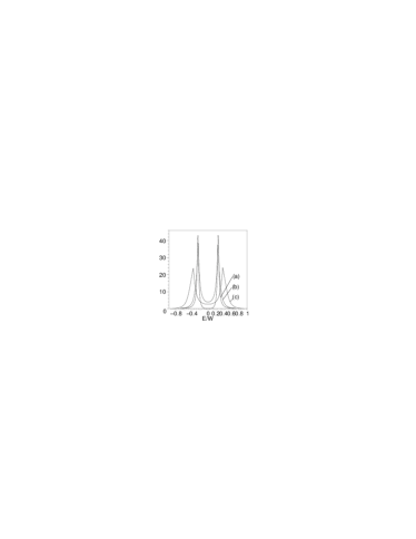
Figure 1: Spectral function $A_{f}(E)\times W$ for different values of the theory parameters as function of energy $E/W$ in the Hubbard I approximation (case (a)) and in the our ladder approximation (cases (b) and (c)). In the cases (a) and (b) $U=1\,eV,\quad W=2\,eV,\quad\Gamma=0.1\,eV$ and in case case (c) $U=1.5\,eV,\quad W=2\,eV,\quad\Gamma=0.15\,eV$.

As can be seen from Figure 1 there are two sharp resonance peaks near the energies $E=\pm E_{0}$ and smooth behaviour near E=0. The distance between peaks is determined by parameter $U$ and the height and width of peaks are determine by parameter $\Gamma$.

IV Conclusions

We discuss the symmetric Anderson impurity model and take into account the strong electronic correlations of the impurity electrons by elaborating the suitable diagram technique. This paper is based on the previous our one^[1] founded on the diagrammatical investigation and analysis of the properties of single-site Anderson model. First of all we establish the antisymmetry property of the functions $g^{0}(i\omega)$, $\Lambda_{\sigma}(i\omega)$ and $g_{\sigma}(i\omega)$, and use the exact Dyson type equations for our functions. The special approximation for the correlation function $Z_{\sigma}(i\omega)$ has been obtained which gives the possibility to close the system of equations and to find the solution for renormalized function $g_{\sigma}(i\omega)$. This Matsubara Green’s function is continued analytically to obtain the retarded one.

Spectral function of impurity electrons is obtained and the structure of resonances and their properties are analyzed. Two of resonances of this function at $E=\pm E_{0}$ (Figure 1) correspond to the energies of quantum transitions of single – site impurity and the smooth behaviour was found at the energy $E=0$. The details of the spectral function renormalization are based on the properties of real $I(E)$ and imaginary $\Gamma(E)$ parts of function $G_{\sigma}^{0}(i\omega)$, which is conduction band electron function averaged by the hybridization interaction. The values of these functions and of the values of energies $\pm E_{0}$ are discussed in a special Appendix.

Appendix A Simple examples of density of states

We can demonstrate some simple examples of the choice of the density of states and of the corresponding functions $I(E)$ and $\Gamma(E)$. For simplicity the energy dependence of the matrix element of hybridization $V(\epsilon)$ is supposed smooth and is neglected. One example of density of states has been proposed in the paper^[4]. In this paper the following equations are used

$$\rho_{0}(\epsilon) = \rho_{0}(0)\left(1-\left(\epsilon/U\right)^{2}\right),\qquad\left|\epsilon\right|<W,$$

$$I(\epsilon) = \rho_{0}(0)V^{2}(0)[2\epsilon/W+\left(\epsilon^{2}/W^{2}-1\right)\ln\left|\frac{\epsilon-W}{\epsilon+W}\right|],$$

$$\Gamma(\epsilon) = \pi V^{2}(\epsilon)\rho_{0}(\epsilon).$$ (37)

where $2W$ is the conduction band width. For little value of energy we have $I(\epsilon)=I^{\prime}(0)\epsilon$  with

$$I^{\prime}(0)=4\rho_{0}(0)V^{2}(0)/W$$ (38)

and for $E\rightarrow\pm\infty$ function $I(E)$ tends to zero as $1/E$. In the case $(A1)$ the equation (26) takes the form $\left(x_{0}=E_{0}/W\right)$:

$$x_{0}-a^{2}/x_{0}-b\varphi(x_{0})=0,$$ (39)

where

$$\varphi(x) = 2x+(x^{2}-1)\ln\left|\frac{x-1}{x+1}\right|;\,\,a=U/2W;\,\,$$

$$b = \rho(0)V^{2}/W.$$

We note that the functions $\rho_{0}(\epsilon)$ and $\Gamma(\epsilon)$ exist only inside the edges of the conduction electron band $\left|E\right|<W$ whereas the function $I(\epsilon)$ and the solution of equation $(A2)$ can exist also for $\left|E\right|>W$. Therefore we have to find the solution of $(A2)$ with $x<1$ and consider the conditions for the values of parameters $a$ and $b$ compatible with this requirement.

Another simple example of the density of state is one with Lorentzian shape^[5]

$$\rho_{0}(\epsilon)=2D/(E^{2}+D^{2}),$$ (40)

with chemical potential placed at the $\epsilon=0$. This choice has the advantage of not introducing band edges. It has the parameter $D$ as an effective band width:

$$I(E) = 2\pi V^{2}(0)E/(E^{2}+D^{2})$$

$$\Gamma(E) = \pi\rho_{0}(0)V^{2}(0)=2\pi V^{2}(0)/D.$$

In this case instead of equation $(A3)$ we have other values of parameters $a$ and $b$ and other form of function $\varphi(x)$:

$$x-a^{2}/x-bx/(1+x^{2}) = 0,$$

$$a=U/2D;\,\,\,b = 2\pi V^{2}(0)/D^{2}.$$

Equation ($A6)$ has two solutions $\pm x_{0}$ with

$$x_{0}=\left[\sqrt{(1-a^{2}+b)^{2}+4a^{2}}+a^{2}+b-1\right]^{1/2}/\sqrt{2}.$$ (43)

The value of parameter $I^{\prime}(0)$ is equal to $2\pi V^{2}(0)/D^{2}=\pi V^{2}(0)\rho_{0}(0)/D.$

References

• (1) V. A. Moskalenko, P. Entel, D. F. Digor and L. A. Dohotaru, Single-site Anderson model. I Diagrammatic theory.
• (2) M. I. Vladimir and V. A. Moskalenko, Theor. Math. Phys. 82, 3301 (1990).
• (3) S. I. Vacaru, M. I. Vladimir and V. A. Moskalenko, Theor. Math. Phys. 57, 1185 (1990).
• (4) A. M. Clogston, Phys. Rev. 125, 439 (1962).
• (5) G. D. Mahan, Many - Particle Physics, Third Edition, Kluwer Academic/Plenum Publisher, New York, ch. 6.