Single-site Anderson Model. I Diagrammatic theory

Abstract

The diagrammatic theory is proposed for the strongly correlated impurity Anderson model. The strongly correlated impurity electrons are hybridized with free conduction electrons. For this system the new diagrammatic approach is formulated. The linked cluster theorem for vacuum diagrams is proved and the Dyson type equations for electron propagators of both electron subsystems are established, together with such equations for mixed propagators. The approximations based on the summing the infinite series of diagrams are proposed, which close the system of equations and permit the investigation of the system’s properties.

I Introduction

The study of strongly-correlated electron systems become in the last decade one of the most active fields of condensed matter physics. The properties of these systems can not be described by Fermi liquid theory. One of the important models of strongly correlated electrons is the single-site or impurity model introduced by Anderson^[1] in the 1961 and discussed intensively in a lot of papers^[2-15]. It is a model for a system of free conduction electrons that interact with the system of local spin, treated as just another electrons of $d$- or $f$- shells of an impurity atom. The impurity electrons are strongly correlated because of strong Coulomb repulsion and they undergo the exchange and hybridization with conduction electrons. This model has some properties similar to those of Kondo model having more interesting physics^[16-18]. It has the application for heavy fermion systems where the local impurity orbital is $f$ - orbital. Investigations of impurity Anderson model have used intensively the methods and results obtained for Kondo model by Nagaoka^[18] and other authors^[19,20]. All the cited papers are based on the method of equation of motions for retarded and advanced quantum Green’s functions proposed by Bogoliubov and Tiablikov^[21] and developed in papers^[22-24].

The first attempt to develop the diagrammatic theory for this problem was realized in the paper^[25]. These authors used the expansion by cumulants for averages of products of Hubbard transfer operators and their algebra.

With introduction of Dynamical Mean Field Theory the interest for Anderson impurity model increases because infinite dimensional lattice models can be mapped onto effective impurity models together with a self-consistency condition^[26,27].

The Hamiltonian of the model is written as

$$H = H_{0}+H_{int},$$

$$H_{0} = H_{0}^{c}+H_{0}^{f},$$

$$H_{0}^{c} = \sum\limits_{\mathbf{k}\sigma}\epsilon(\mathbf{k})\ C_{\mathbf{k}\sigma}^{+}C_{\mathbf{k}\sigma}.$$

$$H_{0}^{f} = \epsilon_{f}\sum\limits_{\sigma}f_{\sigma}^{+}f_{\sigma}+Un_{\uparrow}^{f}n_{\downarrow}^{f},$$ (1)

$$H_{int} = \frac{1}{\sqrt{N}}\sum\limits_{\mathbf{k}\sigma}\left(V_{\mathbf{k}\sigma}f_{\sigma}^{+}C_{\mathbf{k}\sigma}+V_{\mathbf{k}\sigma}^{\ast}C_{\mathbf{k}\sigma}^{+}f_{\sigma}\right),$$

$$n_{\sigma}^{f} = f_{\sigma}^{+}f_{\sigma},$$

where $C_{\mathbf{k}\sigma}(C_{\mathbf{k}\sigma}^{+})$ and $f_{\sigma}(f_{\sigma}^{+})$ - annihilation (creation) operators of conduction and impurity electrons with spin $\sigma$ correspondingly. $\epsilon(\mathbf{k})$ is the kinetic energy of the conduction band state $(\mathbf{k},\sigma)$ , $\epsilon_{f}\$is the local energy of $f$ - electrons, $U$ - is the on-site Coulomb repulsion of the impurity electrons and $N$ is the number of lattice sites. $H_{int}$ is the hybridization interaction between conduction and localized electrons. Summation over $\mathbf{k}$ will be changed to an integral over the energy $\epsilon(\mathbf{k})$ with the density of state $\rho_{0}(\epsilon)$ of conduction electrons and the matrix elements will be considered as the function of energy $V(\epsilon)$. Because of the hybridization term of the Hamiltonian down and up spins of conduction electrons come and go in the local orbital and there is no appearance of spin flip process. Thus the important parameters of the Anderson model are the band width $W$, the conduction density of states $\rho(\epsilon),$ the local site energy $\epsilon_{f}$ and the on-site Coulomb interaction $U$. The electron energies are counted of chemical potential $\mu$ of the system: $\epsilon(\mathbf{k})=\xi(\mathbf{k})-\mu,\qquad\epsilon_{f}=\overline{\epsilon}_{f}-\mu$ . There is also an energy parameter $\Gamma(\epsilon)$ associated with the hybridization term

$$\Gamma(\epsilon)=\frac{\pi}{N}\sum\limits_{\mathbf{k}}V_{\mathbf{k}}^{2}\delta(\epsilon-\epsilon(\mathbf{k}))=\pi V^{2}(\epsilon)\rho_{0}(\epsilon).$$ (2)

This function is assumed to be a constant, independent of energy. The term in the Hamiltonian involving $U$ comes from on-site Coulomb interaction between two impurity electrons. $U$ it is far to large to be treated by perturbation theory. It must be included in $Ho$ which is non interacting Hamiltonian. The existence of this term invalidates Wick’s theorem for local electrons. Therefore, first of all, we formulate the generalized Wick’s theorem (GWT) for local electrons, preserving the ordinary Wick theorem for conduction electrons. Our GWT really is the identity which determines the irreducible Green’s functions or Kubo cumulants. Such definitions have already been used by us for discussing the properties of one-band Hubbard model^[28-30] and the formulation of the new diagram technique for it^[31-34].

In Section II, we start by introducing the temperature Green’s functions for the conduction and impurity electrons in interaction representation, formulate the generalized Wick theorem and provide explicit examples of diagram calculation for thermodynamical potential and full propagators. The results are analyzed in Section III and compared to the other data in Section IV. Some approximations are discussed in Section V and in Section VI there are the conclusions.

II Diagrammatical theory

The Matsubara renormalized Green’s functions of conduction and impurity electrons in interaction representation have the form:

$$G(\mathbf{k,}\sigma,\tau\mid\mathbf{k}^{\prime},\sigma,^{\prime}\tau^{\prime}) = -\ \left\langle TC_{\mathbf{k}\sigma}(\tau)\overline{C}_{\mathbf{k}^{\prime}\sigma^{\prime}}(\tau^{\prime})U(\beta)\right\rangle_{0}^{c},$$

$$g(\sigma,\tau\mid\sigma^{\prime},\tau^{\prime}) = -\ \left\langle Tf_{\sigma}(\tau)\overline{f}_{\sigma^{\prime}}(\tau^{\prime})U(\beta)\right\rangle_{0}^{c}.$$ (3)

Besides them there are also anomalous ones:

$$F(\mathbf{k,}\sigma,\tau\mid-\mathbf{k,}-\sigma^{\prime},\tau^{\prime}) = -\ \left\langle TC_{\mathbf{k}\sigma}(\tau)C_{-\mathbf{k}^{\prime}-\sigma^{\prime}}(\tau^{\prime})U(\beta)\right\rangle_{0}^{c},$$

$$\overline{F}(-\mathbf{k,}-\sigma,\tau\mid\mathbf{k}^{\prime},\sigma^{\prime},\tau^{\prime}) = -\ \left\langle T\overline{C}_{-\mathbf{k}-\sigma}(\tau)\overline{C}_{\mathbf{k}^{\prime}\sigma^{\prime}}(\tau^{\prime})U(\beta)\right\rangle_{0}^{c},$$

$$f(\sigma,\tau\mid-\sigma^{\prime},\tau^{\prime}) = -\ \left\langle Tf_{\sigma}(\tau)f_{-\sigma^{\prime}}(\tau^{\prime})U(\beta)\right\rangle_{0}^{c},$$

$$\overline{f}(-\sigma,\tau\mid\sigma^{\prime},\tau^{\prime}) = -\ \left\langle T\overline{f}_{-\sigma}(\tau)\overline{f}_{\sigma^{\prime}}(\tau^{\prime})U(\beta)\right\rangle_{0}^{c},$$

(4)

if the system is in superconducting state. Here $\tau$ and $\tau^{\prime}$ stand for imaginary time with $0<\tau<\beta$, $\beta$ - inverse temperature and T is the chronological ordering operator. The evolution operator $U(\beta)$ is given by

$$U(\beta) = T\exp(-\int\limits_{0}^{\beta}H_{int}(\tau)d\tau)=\sum\limits_{n=0}^{\infty}\frac{(-1)^{n}}{n!}\int\limits_{0}^{\beta}d\tau_{1}...\int\limits_{0}^{\beta}d\tau_{n}T(H_{int}(\tau_{1})...H_{int}(\tau_{n})).$$ (5)

The statistical averaging is carried out in (3) and (4) with respect to the zero-order density matrix of the conduction and impurity electrons.

$$\frac{e^{-\beta H_{0}}}{Tre^{-\beta H_{0}}}=\frac{e^{-\beta H_{0}^{c}}}{Tre^{-\beta H_{0}^{c}}}\times\frac{e^{-\beta H_{0}^{f}}}{Tre^{-\beta H_{0}^{f}}}.$$ (6)

The thermodynamic perturbation theory for $H_{int}$ requires the generalization adequate for calculation of the statistical averages of the $T\$- products of localized $f$ - electron operators. This necessity appears for the reason that cannot be diagonalized with free $f$ - electron operators. This Hamiltonian can be diagonalized by using the algebra of Hubbard^[28-30] transfer operators $\chi^{mn}=\left|m><n\right|$ when the $\mid$$m$$>$ with $m=-1,0,1,2$ enumerates four states of the impurity atom: $\mid$$0>$ - is the empty or vacuum state with energy $E_{0}=0$, the $\mid$$1>$ and $\mid$$-1>$ or $\mid$ $\uparrow>$ and $\mid$$\downarrow>$ are the states with one particle with energy $E_{\sigma}=\epsilon_{f}$ and spin $\sigma=\pm 1$ and the state $\mid$$2>=\mid$$\uparrow\downarrow>$ contains two $f$ - electrons with opposite spins and the energy $E_{2}=U+2\epsilon_{f}$. By using the relation

$$f_{\sigma}=\chi^{0\sigma}+\sigma\chi^{\overline{\sigma}2},$$ (7)

we obtain the diagonalized form of the impurity Hamiltonian

$$H_{0}^{f}=\sum\limits_{n=-1}^{2}E_{n}\chi^{nn},\qquad\sum\limits_{n=-1}^{2}\chi^{nn}=1.$$ (8)

In zero order approximation, when we neglect the process of hybridization of the conduction and impurity electrons, the corresponding Green’s functions have the form $(\omega\equiv\omega_{n}=(2n+1)\pi/\beta)$

$$G_{\sigma\sigma^{\prime}}^{0}(\mathbf{k},\mathbf{k}^{\prime}\mid i\omega) = \delta_{\sigma\sigma^{\prime}}\delta_{\mathbf{kk}^{\prime}}\frac{1}{i\omega-\epsilon(\mathbf{k)}},$$

$$g_{\sigma\sigma^{\prime}}^{0}=\delta_{\sigma\sigma^{\prime}}g_{\sigma}^{0}(i\omega) = \frac{1-n_{\overline{\sigma}}}{\lambda_{\sigma}(i\omega)}+\frac{n_{\overline{\sigma}}}{\overline{\lambda}_{\overline{\sigma}}(i\omega)},$$ (9)

where $(\overline{\sigma}=-\sigma)$

$$\lambda_{\sigma}(i\omega) = i\omega+E_{0}-E_{\sigma}$$

$$\overline{\lambda}_{\overline{\sigma}}(i\omega) = i\omega+E_{\overline{\sigma}}-E_{2},$$

$$Z_{0} = e^{-\beta E_{0}}+e^{-\beta E_{\sigma}}+e^{-\beta E_{\overline{\sigma}}}+e^{-\beta E_{2}},$$

$$n_{\overline{\sigma}} = \frac{e^{-\beta E_{\overline{\sigma}}}+e^{-\beta E_{2}}}{Z_{0}},$$

$$1-n_{\overline{\sigma}} = \frac{e^{-\beta E_{0}}+e^{-\beta E_{\sigma}}}{Z_{0}}.$$

In the case of $f$ - electrons we formulate the identity which is just our GWT in this simple case:

$$\left\langle Tf_{1}f_{2}\overline{f}_{3}\overline{f}_{4}\right\rangle_{0} = \left\langle Tf_{1}\overline{f}_{4}\right\rangle_{0}\left\langle Tf_{2}\overline{f}_{3}\right\rangle_{0}-\left\langle Tf_{1}\overline{f}_{3}\right\rangle_{0}\left\langle Tf_{2}\overline{f}_{4}\right\rangle_{0}+\left\langle Tf_{1}f_{2}\overline{f}_{3}\overline{f}_{4}\right\rangle_{0}^{ir},$$ (10)

or

$$g_{2}^{0}(1,2|3,4) = g^{0}(1|4)g^{0}(2|3)-g^{0}(1|3)g^{0}(2|4)+g_{2}^{(0)ir}(1,2|3,4),$$ (11)

where $n$ stands for $(\sigma_{n},\tau_{n})$. The generalization for more complicate averages of type
$g_{n}^{0}(1,...,n\mid n+1,...,2n)=(-1)^{n}\left\langle Tf_{1}...f_{n}\overline{f}_{n+1}...\overline{f}_{2n}\right\rangle_{0}$ is straightforward, namely the right - hand part of this quantity will contain $n!$ term of ordinary Wick type (chain diagrams) and also the different products of irreducible functions with the same total number of operators. The full irreducible functions in
$g_{n}^{0}(1,...,n|n+1,...,2n)$ also appears. For example $g_{3}^{0}(123|456)$ contains the contribution of $3!=6$ terms of ordinary Wick kind, then appear 9 terms of the form $g^{0}(1|4)g_{2}^{(0)ir}(23|56)$ and the last term is $g_{3}^{(0)ir}(123|456)$ . The total number of terms is 16. In the case of $g_{4}^{0}(1234|5678)$ there are $4!=24$ terms of ordinary Wick kind, the 72 terms of the type $g^{0}(1|5)g^{0}(2|6)g_{2}^{(0)ir}(34|78)$, then 18 terms of type $g_{2}^{(0)ir}(12|56)g_{2}^{(0)ir}(34|78)$, then 16 terms of the form $g^{0}(1|5)g_{3}^{(0)ir}(234|678)$ and finally one form $g_{4}^{(0)ir}(1234|5678)$. The total number of terms is 131. The signs of all these contributions can be easily determined. Thus the definition of the irreducible Green’s functions or Kubo cumulants is just our GWT. In the absence of Coulomb repulsion $U\$all these irreducible functions are equal to zero. When $U\neq 0$ they contain all the spin, charge and pairing fluctuations produced by the strong correlations. These definitions are the simplification of ones for Hubbard and other lattice models. The calculation of the simplest irreducible functions for example $g_{2}^{(0)ir}(12|34)$ is rather cumbersome but straightforward. It is necessary to find the values of chronological averages for $4!=24$ different orders of $\tau_{1},\tau_{2},\tau_{3}$ and $\tau_{4}$ times and then to determine its Fourier representation

$$g_{2}^{(0)ir}[\sigma_{1},\tau_{1};\sigma_{2},\tau_{2}|\sigma_{3},\tau_{3};\sigma_{4},\tau_{4}] = \frac{1}{\beta^{4}}\sum\limits_{\omega_{1}\omega_{2}\omega_{3}\omega_{4}}\exp(-i\omega_{1}\tau_{1}-i\omega_{2}\tau_{2}+i\omega_{3}\tau_{3}+i\omega_{4}\tau_{4})\times$$

$$\times g_{2}^{(0)ir}[\sigma_{1},i\omega_{1};\sigma_{2},i\omega_{2}|\sigma_{3},i\omega_{3};\sigma_{4},i\omega_{4}].$$

The Fourier representation conserves the frequencies

$$g_{2}^{(0)ir}[\sigma_{1},i\omega_{1};\sigma_{2},i\omega_{2}|\sigma_{3},i\omega_{3};\sigma_{4},i\omega_{4}] = \beta\delta(\omega_{1}+\omega_{2}-\omega_{3}-\omega_{4})\times$$

$$\times \widetilde{g}_{2}^{(0)ir}[\sigma_{1},i\omega_{1};\sigma_{2},i\omega_{2}|\sigma_{3},i\omega_{3};\sigma_{4},i\omega_{1}+i\omega_{2}-i\omega_{3}].$$

There is also the spin conservation $\sigma_{1}+\sigma_{2}=\sigma_{3}+\sigma_{4}$. Thus we have the rules to deal with chronological averages of thermodynamic perturbation theory.

III Thermodynamic potential

First of all we can determine the thermodynamic potential $F$ of the system

$$F = F_{0}-\frac{1}{\beta}\ln\left\langle U(\beta)\right\rangle_{0},$$

$$F_{0} = -\frac{1}{\beta}\ln Z_{0}-\frac{2}{\beta}\sum\limits_{\mathbf{k}}\ln\left[1+\exp(-\beta\epsilon(\mathbf{k)})\right],$$

where $Zo$ refers to the free impurity atom. The diagrams which determine the thermodynamic potential have not the external lines and are named vacuum.

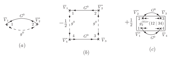
Figure 1: The simplest connected vacuum diagrams in normal state. The diagram $a)$ is of second and $b)$, $c)$ of fourth order of the theory. Here $\overline{V}_{n}=V_{n}/\sqrt{N}$.

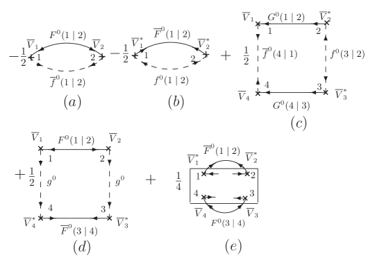
Figure 2: The simplest vacuum anomalous diagrams. The diagrams $a)$ and $b)$ are of second and $c)$, $d)$ and $e)$ of fourth order of perturbation theory.

In $Fig.1$ are shown the simplest vacuum connected diagrams of the normal state. In the diagrams we shall depict the process of hybridization of $C$ and $f$ electrons. The zero order propagators of conduction and impurity electrons are represented by their solid and dashed lines correspondingly. These lines connect the crosses which depict the impurity states. To crosses are attached two arrows, one of which is ingoing and other outgoing. They depict the annihilation and creation electrons correspondingly. The index $n$  means $(\sigma_{n},\tau_{n})$ for impurity and $(\mathbf{k}_{n},\sigma_{n},\tau_{n})$ for conduction electrons. The rectangles with $2n$ crosses depict the irreducible $g_{n}^{(0)ir}$ Green’s functions.

Besides the vacuum diagrams of fourth order shown on the $Fig.1$   $b)$ and $c)$ there is also one disconnected diagram composed from two diagrams of the type $Fig.1$  $a)$  and containing additional factor  $1/2!$. Such situation is repeated in high order of perturbation theory and permit us to formulate linked cluster theorem. It has the form

$$\left\langle U(\beta)\right\rangle_{0}=\exp\left\langle U(\beta)\right\rangle_{0}^{c},$$ (15)

where $\left\langle U(\beta)\right\rangle_{0}^{c}$ contains only connected diagrams and is equal to zero when hybridization is absent. If we admit the existence of the pairing mechanism of conduction electrons, thanks the hybridization, the paring mechanism appear also for impurity electrons. This mechanism results in appearance of the anomalous propagators of both kind of electrons.

$Fig.2$ shows some of the simplest connected anomalous vacuum diagrams. The anomalous propagators are depicted by the thin (solid and dashed) lines with two opposite directions at the end of them.

Figure 3: Second order perturbation theory contribution for conduction electron normal propagator.

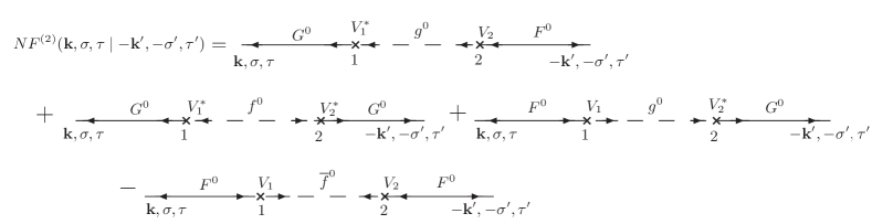
Figure 4: Second order perturbation theory contribution for conduction electron anomalous propagator.

IV Renormalized propagators

Now we shall consider the diagrammatical analysis of the perturbation series for renormalized propagators (3) and (4). The simplest contributions to such series are represented on the $Figures\ 3-6$. All such diagrams contain two external points with attached arrows determined by the arguments of Green’s functions and their kind.On the inner points of diagrams is supposed summation on $\sigma_{n},\mathbf{k}_{n}$, and integration on $\tau_{n}$.

In the same second order approximation of perturbation theory the diagrams for impurity electron propagators contain new diagrammatical elements namely the irreducible two particle Green’s functions. These functions also can be normal or anomalous. The process of their renormalization will be not considered by us, supposing the necessity of renormalization only for the propagators.

In $Fig.5$ the diagrams for impurity electron normal propagator are shown.

The last two irreducible Green’s functions of $Fig.5$ are anomalous ones because they contain non equal number of annihilation and creation $f$-operators enumerated in the left and right parts about the vertical bare correspondingly. Thanks the summation of infinite series diagrams the renormalized normal and anomalous propagators appear and now it is necessary to put equal to zero the source of electron pairs and simultaneously the bare $f^{0}$ and $\overline{f}^{0}$ together with anomalous irreducible Green’s functions. The corresponding contribution to the anomalous impurity electron function $f_{\sigma\sigma^{\prime}}(\tau-\tau^{\prime})$ is depicted on the $Fig.6$

The final equations for renormalized functions it is more convenient to write down in Fourier representation

$$G(\mathbf{k,}\sigma,\tau|\mathbf{k}^{\prime},\sigma^{\prime},\tau^{\prime}) = \frac{1}{\beta}\sum\limits_{\omega}G_{\sigma\sigma^{\prime}}(\mathbf{k},\mathbf{k}^{\prime}|\,i\omega)\,\exp\left[-i\omega(\tau-\tau^{{}^{\prime}})\right],$$

$$F(\mathbf{k,}\sigma,\tau|-\mathbf{k}^{\prime},-\sigma^{\prime},\tau^{\prime}) = \frac{1}{\beta}\sum\limits_{\omega}F_{\sigma\overline{\sigma}^{\prime}}(\mathbf{k},-\mathbf{k}^{\prime}|\,i\omega)\exp\left[-i\omega(\tau-\tau^{{}^{\prime}})\right].$$

The complete equations for the conduction electrons propagators have the form:

$$G_{\sigma\sigma^{\prime}}(\mathbf{k},\mathbf{k}^{\prime}|\,i\omega) = \delta_{\mathbf{kk}^{\prime}}\delta_{\sigma\sigma^{\prime}}G_{\sigma}^{0}(\mathbf{k}|\,i\omega)+\frac{V_{\mathbf{k}}^{\ast}V_{\mathbf{k}^{\prime}}}{N}(G_{\sigma}^{0}(\mathbf{k}|i\omega)g_{\sigma\sigma^{\prime}}(i\omega)G_{\sigma^{\prime}}^{0}(\mathbf{k}^{\prime}|i\omega)-$$ (16)

$$- G_{\sigma}^{0}(\mathbf{k}|i\omega)f_{\sigma\overline{\sigma}^{\prime}}(i\omega)\overline{F}_{\overline{\sigma}^{\prime}\sigma^{\prime}}^{0}(-\mathbf{k}^{\prime}|i\omega))-F_{\sigma\overline{\sigma}}^{0}(\mathbf{k}|i\omega)g_{\overline{\sigma}^{\prime}\overline{\sigma}}(-i\omega)\overline{F}_{\overline{\sigma}^{\prime}\sigma^{\prime}}^{0}(-\mathbf{k}|i\omega)-$$

$$- F_{\sigma\overline{\sigma}}^{0}(\mathbf{k}|i\omega)\overline{f}_{\overline{\sigma}\sigma^{\prime}}(i\omega)G_{\sigma^{\prime}}^{0}(\mathbf{k}^{\prime}|i\omega)),$$

$$F_{\sigma\overline{\sigma}^{\prime}}(\mathbf{k},-\mathbf{k}^{\prime}|\,i\omega) = F_{\sigma\overline{\sigma}}^{0}(\mathbf{k}|\,i\omega)\delta_{\mathbf{kk}^{\prime}}\delta_{\sigma\sigma^{\prime}}+\frac{V_{\mathbf{k}}^{\ast}V_{\mathbf{k}^{\prime}}}{N}(G_{\sigma}^{0}(\mathbf{k}|i\omega)g_{\sigma\sigma^{\prime}}(i\omega)F_{\sigma^{\prime}\overline{\sigma}^{\prime}}^{0}(\mathbf{k}^{\prime}|i\omega)+$$ (17)

$$+ G_{\sigma}^{0}(\mathbf{k}|i\omega)f_{\sigma\overline{\sigma}^{\prime}}(i\omega)G_{\overline{\sigma}^{\prime}}^{0}(-\mathbf{k}^{\prime}|-i\omega)+F_{\sigma\overline{\sigma}}^{0}(\mathbf{k}|i\omega)g_{\overline{\sigma}^{\prime}\overline{\sigma}}(-i\omega)G_{\overline{\sigma}^{\prime}}^{0}(-\mathbf{k}^{\prime}|-i\omega)-$$

$$- F_{\sigma\overline{\sigma}}^{0}(\mathbf{k}|i\omega)\overline{f}_{\overline{\sigma}\sigma^{\prime}}(i\omega)F_{\sigma^{\prime}\overline{\sigma}^{\prime}}^{0}(\mathbf{k}^{\prime}|i\omega)).$$

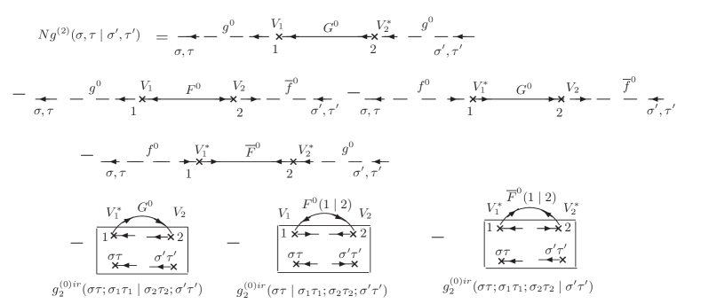
Figure 5: The second order perturbation contribution for the impurity electron normal propagator.

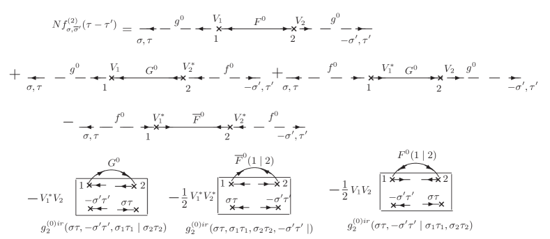
Figure 6: Anomalous impurity electron Green’s function in the second order perturbation theory.

These renormalized propagators are expressed through the full propagators $g,f$ and $\overline{f}$ of impurity electrons. Now it is necessary to obtain the corresponding equations for the full impurity electron propagators. Because the subsystem of $f$-electrons is strongly correlated we have to introduce the correlation functions $Z_{\sigma\sigma^{\prime}},Y_{\sigma\overline{\sigma}^{\prime}}$ and $\overline{Y}_{\overline{\sigma}\sigma^{\prime}}$ which are represented by strong connected diagrams with irreducible Green’s functions^[31-35]. The process of renormalization of $f$-electron propagators is shown on the $Figures$ $7$ and $8$, where the double dashed lines depict the full $f$-electron functions and the rectangles represent the correlation functions $\Lambda_{\sigma\sigma^{\prime}}=g_{\sigma\sigma^{\prime}}^{0}+Z_{\sigma\sigma^{\prime}}$, $Y_{\sigma\sigma^{\prime}}$ and $\overline{Y}_{\overline{\sigma}\sigma}$:

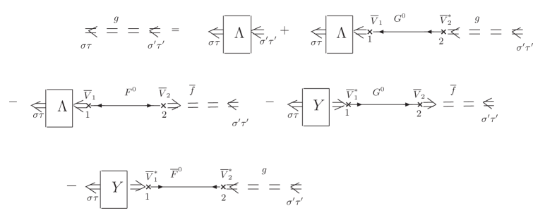
Figure 7: Dyson type equation for the normal propagator of impurity electrons. Double dashed lines depict full electron propagators. The arrows on them distinguish the normal and anomalous ones. The squares with attached arrows depict the correlated functions. On double repeated indices 1 and 2 is supposed summation by $\sigma_{n}$ and $\mathbf{k}_{n}$ and integration by  $\tau_{n}$ .

The second equation we shall depict for anomalous propagator $\overline{f}$ of the impurity electrons (see $Fig.8$).

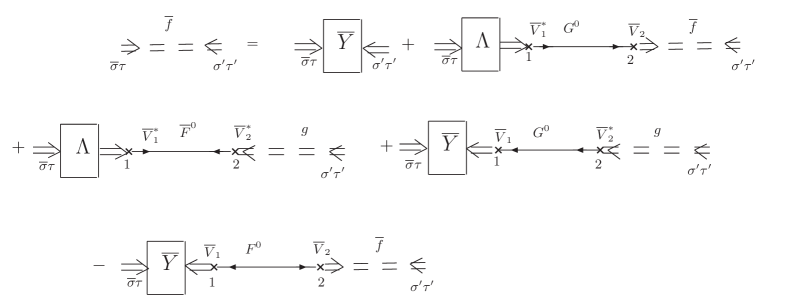
Figure 8: Dyson type equation for one of anomalous Green’s functions of $f$ -electrons.

In both these equations the bare conduction electron propagators $G_{\sigma}^{0}(\mathbf{k}|i\omega)$, $F_{\sigma\overline{\sigma}}^{0}(\mathbf{k}|i\omega)$ and
$\overline{F}_{\overline{\sigma}\sigma}^{0}(-\mathbf{k}|i\omega)$ play the role of mass operators for the $f$-electron propagators. It is easy to see that these functions participate in above equations being averaged on the Brillouin cell with matrix elements of hybridization. Therefore we define the new quantities

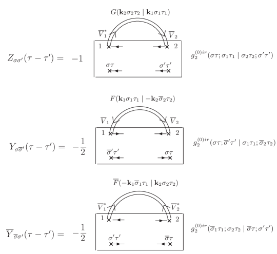
Figure 9: Schematic representation of the main approximations for the correlated functions The solid double lines with arrows depict the renormalized one-particle Green’s functions of conduction electrons. The rectangles depict the irreducible Green’s functions of impurity electrons.

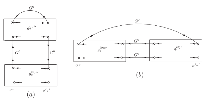
Figure 10: Examples of the simplest ladder diagram for $g$-function.

$$\frac{1}{N}\sum\limits_{\mathbf{k}_{1}\mathbf{k}_{2}}V_{\mathbf{k}_{2}}^{\ast}V_{\mathbf{k}_{1}}G^{0}(\mathbf{k}_{1},\sigma_{1},\tau_{1}|\mathbf{k}_{2},\sigma_{2},\tau_{2}) = \frac{1}{N}\sum\limits_{\mathbf{k}_{1}}\,|V_{\mathbf{k}_{1}}|^{2}G_{\sigma_{1}\sigma_{2}}^{0}(\mathbf{k}|\tau_{1}-\tau_{2})\equiv\delta_{\sigma_{1}\sigma_{2}}G_{\sigma_{1}}^{0}(\tau_{1}-\tau_{2}),$$

$$\frac{1}{N}\sum\limits_{\mathbf{k}_{1}\mathbf{k}_{2}}V_{\mathbf{k}_{1}}^{\ast}V_{\mathbf{k}_{2}}^{\ast}\overline{F}^{0}(\mathbf{k}_{1},\overline{\sigma}_{1},\tau_{1}|\mathbf{k}_{2},\sigma_{2},\tau_{2}) = \frac{1}{N}\sum\limits_{\mathbf{k}_{1}}\,|V_{\mathbf{k}_{1}}|^{2}\overline{F}_{\overline{\sigma}_{1}\sigma_{2}}^{0}(-\mathbf{k}_{1}|\tau_{1}-\tau_{2})\equiv\delta_{\sigma_{1}\sigma_{2}}\overline{F}_{\overline{\sigma}_{1}\sigma_{1}}^{0}(\tau_{1}-\tau_{2}),$$ (18)

$$\frac{1}{N}\sum\limits_{\mathbf{k}_{1}\mathbf{k}_{2}}V_{\mathbf{k}_{1}}V_{\mathbf{k}_{2}}F^{0}(\mathbf{k}_{1},\sigma_{1},\tau_{1}|\mathbf{k}_{2},\overline{\sigma}_{2},\tau_{2}) = \frac{1}{N}\sum\limits_{\mathbf{k}_{1}}\,|V_{\mathbf{k}_{1}}|^{2}F_{\sigma_{1}\overline{\sigma}_{2}}^{0}(\mathbf{k}_{1}|\tau_{1}-\tau_{2})\equiv\delta_{\sigma_{1}\sigma_{2}}F_{\sigma_{1}\overline{\sigma}_{1}}^{0}(\tau_{1}-\tau_{2}).$$

These definitions gives us the possibility to simplify the structure of equations for the $f$-electron propagators. By using these average bare propagators $G_{\sigma}^{0}$, $F_{\sigma\overline{\sigma}}^{0}$ and $\overline{F}_{\overline{\sigma}\sigma}^{0}$ and Fourier representation for $\tau$-variables we obtain

$$g_{\sigma}(i\omega) = \frac{\Lambda_{\sigma}(i\omega)\,\,-\,\,G_{\overline{\sigma}}^{0}(-i\omega)[\Lambda_{\sigma}(i\omega)\Lambda_{\overline{\sigma}}(-i\omega)\,\,+\,\,Y_{\sigma\overline{\sigma}}(i\omega)\overline{Y}_{\overline{\sigma}\sigma}(i\omega)]}{d_{\sigma}(i\omega)},$$ (19)

$$\overline{f}_{\overline{\sigma}\sigma}(i\omega) = \frac{\overline{Y}_{\overline{\sigma}\sigma}(i\omega)\,\,+\,\,\overline{F}_{\overline{\sigma}\sigma}^{0}(i\omega)(\Lambda_{\sigma}(i\omega)\Lambda_{\overline{\sigma}}(-i\omega)\,\,+\,\,Y_{\sigma\overline{\sigma}}(i\omega)\overline{Y}_{\overline{\sigma}\sigma}(i\omega))}{d_{\sigma}(i\omega)},$$ (20)

$$f_{\sigma\overline{\sigma}}(i\omega) = \frac{\{Y_{\sigma\overline{\sigma}}(i\omega)\,\,+\,F_{\sigma\overline{\sigma}}^{0}(i\omega)[(\Lambda_{\sigma}(i\omega)\Lambda_{\overline{\sigma}}(-i\omega)\,\,+\,\,Y_{\sigma\overline{\sigma}}(i\omega)\overline{Y}_{\overline{\sigma}\sigma}(i\omega)]\}}{d_{\sigma}(i\omega)},$$ (21)

$$d_{\sigma}(i\omega) = (1-\Lambda_{\sigma}(i\omega)G_{\sigma}^{0}(i\omega))(1-\Lambda_{\overline{\sigma}}(-i\omega)G_{\overline{\sigma}}^{0}(-i\omega))+\overline{Y}_{\overline{\sigma}\sigma}(i\omega)F_{\sigma\overline{\sigma}}^{0}(i\omega)+$$ (22)

$$+ Y_{\sigma\overline{\sigma}}(i\omega)\overline{F}_{\overline{\sigma}\sigma}^{0}(i\omega)+\overline{F}_{\overline{\sigma}\sigma}^{0}(i\omega)F_{\sigma\overline{\sigma}}^{0}(i\omega)[Y_{\sigma\overline{\sigma}}(i\omega)\overline{Y}_{\overline{\sigma}\sigma}(i\omega)+\Lambda_{\sigma}(i\omega)\Lambda_{\overline{\sigma}}(-i\omega)]+$$

$$+ G_{\overline{\sigma}}^{0}(-i\omega)G_{\sigma}^{0}(i\omega)Y_{\sigma\overline{\sigma}}(i\omega)\overline{Y}_{\overline{\sigma}\sigma}(i\omega).$$

In the previous part of the paper we supposed the existence of pairing potential of conduction electrons with order parameter and with the bare propagators:

$$G_{\sigma}^{0}(\mathbf{k}|i\omega) = \frac{i\omega\,+\,\epsilon(\mathbf{k})}{(i\omega)^{2}-E^{2}(\mathbf{k})};\,\,F_{\sigma\overline{\sigma}}^{0}(\mathbf{k}|i\omega)=\overline{F}_{\overline{\sigma}\sigma}^{0}(-\mathbf{k}|i\omega)=\frac{\Delta}{(i\omega)^{2}-\,E^{2}(\mathbf{k})};\,\,E(\mathbf{k})=\sqrt{\epsilon^{2}(\mathbf{k})+\Delta^{2}}.$$ (23)

Now we shall discuss the case when the pairing potential is absent and the superconducting state appears simultaneously  with both subsystems as a consequence of the broken symmetry and phase transition. In this more simple case the renormalized conduction electron propagators have the form

$$G_{\sigma\sigma^{\prime}}(\mathbf{k},\mathbf{k}|i\omega) = \delta_{\mathbf{kk}}\delta_{\sigma\sigma^{\prime}}G_{\sigma}^{0}(\mathbf{k}|i\omega)+\frac{V_{\mathbf{k}}^{\ast}V_{\mathbf{k}}}{N}G_{\sigma}^{0}(\mathbf{k}|i\omega)g_{\sigma\sigma^{\prime}}(i\omega)G_{\sigma^{\prime}}^{0}(\mathbf{k}|i\omega),$$ (24)

$$F_{\sigma\overline{\sigma}^{\prime}}(\mathbf{k},-\mathbf{k}|i\omega) = \frac{V_{\mathbf{k}}^{\ast}V_{\mathbf{k}}}{N}G_{\sigma}^{0}(\mathbf{k}|i\omega)f_{\sigma\overline{\sigma}^{\prime}}(i\omega)G_{\overline{\sigma}^{\prime}}^{0}(-\mathbf{k}|-i\omega),$$ (25)

$$G_{\sigma}^{0}(\mathbf{k}|i\omega) = (i\omega-\epsilon(\mathbf{k}))^{-1}.$$ (26)

The renormalized propagators of impurity electron in this case are:

$$g_{\sigma}(i\omega) = \frac{\Lambda_{\sigma}(i\omega)\,\,-\,\,G_{\overline{\sigma}}^{0}(-i\omega)[\Lambda_{\sigma}(i\omega)\Lambda_{\overline{\sigma}}(-i\omega)\,\,+\,\,Y_{\sigma\overline{\sigma}}(i\omega)\overline{Y}_{\overline{\sigma}\sigma}(i\omega)]}{d_{\sigma}(i\omega)},$$ (27)

$$\overline{f}_{\overline{\sigma}\sigma}(i\omega) = \frac{\overline{Y}_{\overline{\sigma}\sigma}(i\omega)\,\,}{d_{\sigma}(i\omega)};\,\,f_{\sigma\overline{\sigma}}(i\omega)=\frac{Y_{\sigma\overline{\sigma}}(i\omega)\,\,}{d_{\sigma}(i\omega)},$$ (28)

$$d_{\sigma}(i\omega) = (1-\Lambda_{\sigma}(i\omega)G_{\sigma}^{0}(i\omega))(1-\Lambda_{\overline{\sigma}}(-i\omega)G_{\overline{\sigma}}^{0}(-i\omega))+$$ (29)

$$+ G_{\overline{\sigma}}(-i\omega)G_{\sigma}^{0}(i\omega)Y_{\sigma\overline{\sigma}}(i\omega)\overline{Y}_{\overline{\sigma}\sigma}(i\omega).$$

The equation (24) has been established many years ago in the paper of Anderson^[1] by using the equation of motion of conduction electron operators. In this equation the propagator $g_{\sigma}(i\omega)$ has the role of $t$-matrix for non-spin-flip scattering. By setting $\mathbf{k}=\mathbf{k}^{\prime}$ in $G_{\sigma}(\mathbf{k},\mathbf{k}^{\prime}|i\omega)$

$$G_{\sigma}(\mathbf{k},\mathbf{k}^{\prime}|i\omega)=\frac{1}{i\omega\,-\,\epsilon(\mathbf{k})}+\frac{|V_{\mathbf{k}}|^{2}g_{\sigma}(i\omega)}{N(i\omega\,-\,\epsilon(\mathbf{k}))^{2}}$$ (30)

and considering the Lehmann spectral representation it is possible to conclude that the discontinuity of $g_{\sigma}(E)$ across the real axis is pure imaginary^[8]

$$g_{\sigma}(E+i\delta)=[g_{\sigma}(E-i\delta)]^{\ast}.$$ (31)

The Green’s function $g_{\sigma}(i\omega)$ has been known till now in approximate form as a result of special decoupling mechanism used for equation of motion of quantum Green’s functions. As is known in such decoupling approximation some combinations of operators is taken off the average value of product of operators and are replaced by their average values. After that truncation the Green’s functions of low order remain. This approximation has been proposed by Bogoliubov, Tiablikov, Zubarev and Tserkovnikov^[21-24] and used by other authors^[2-14,18]. The hybridization of conduction and impurity electrons causes the appearance of mixed Green’s functions:

$$G_{m}(\mathbf{k},\sigma,\tau|\sigma^{\prime},\tau^{\prime}) = -\left\langle TC_{\mathbf{k}\sigma}(\tau)\overline{f}_{\sigma^{\prime}}(\tau^{\prime})U(\beta)\right\rangle_{0}^{c},$$

$$F_{m}(\mathbf{k},\sigma,\tau|\overline{\sigma}^{\prime},\tau^{\prime}) = -\left\langle TC_{\mathbf{k}\sigma}(\tau)f_{\overline{\sigma}^{\prime}}(\tau^{\prime})U(\beta)\right\rangle_{0}^{c},\qquad$$ (32)

$$\overline{F}_{m}(-\mathbf{k},\overline{\sigma},\tau|\sigma^{\prime},\tau^{\prime}) = -\left\langle T\overline{C}_{-\mathbf{k}\overline{\sigma}}(\tau)\overline{f}_{\sigma^{\prime}}(\tau^{\prime})U(\beta)\right\rangle_{0}^{c},$$

and also

$$G^{m}(\sigma,\tau|\mathbf{k},\sigma^{\prime},\tau^{\prime}) = -\left\langle Tf_{\sigma}(\tau)\overline{C}_{\mathbf{k}\sigma^{\prime}}(\tau^{\prime})U(\beta)\right\rangle_{0}^{c},$$

$$F^{m}(\sigma,\tau|-\mathbf{k},\overline{\sigma}^{\prime},\tau^{\prime}) = -\left\langle Tf_{\sigma}(\tau)C_{-\mathbf{k}\overline{\sigma}^{\prime}}(\tau^{\prime})U(\beta)\right\rangle_{0}^{c},$$ (33)

$$\overline{F}^{m}(\overline{\sigma},\tau|\mathbf{k},\sigma^{\prime},\tau^{\prime}) = -\left\langle T\overline{f}_{\overline{\sigma}}(\tau)\overline{C}_{\mathbf{k}\sigma^{\prime}}(\tau^{\prime})U(\beta)\right\rangle_{0}^{c}.$$

Let $G_{m\sigma\sigma^{\prime}}(\mathbf{k}|i\omega)$, $F_{m\sigma\overline{\sigma}^{\prime}}(\mathbf{k}|i\omega)$ and $F_{m\overline{\sigma}\sigma^{\prime}}(\mathbf{k}|i\omega)$ be the Fourier representation of the first group of Green’s functions and $G_{\sigma\sigma^{\prime}}^{m}(\mathbf{k}|i\omega)$, $F_{\sigma\overline{\sigma}^{\prime}}^{m}(-\mathbf{k}|i\omega)$ and $\overline{F}_{\overline{\sigma}\sigma^{\prime}}^{m}(\mathbf{k}|i\omega)$ of the second group.
In the presence of superconducting pairing of conduction electrons we obtain the following results:

$$G_{m\sigma\sigma^{\prime}}(\mathbf{k}|i\omega) = \frac{V_{\mathbf{k}}^{\ast}}{\sqrt{N}}\left[G_{\sigma}^{0}(\mathbf{k}|i\omega)g_{\sigma\sigma^{\prime}}(i\omega)-F_{\sigma\overline{\sigma}}^{0}(\mathbf{k}|i\omega)\overline{f}_{\overline{\sigma}\sigma^{\prime}}(i\omega)\right],$$

$$F_{m\sigma\overline{\sigma}^{\prime}}(\mathbf{k}|i\omega) = \frac{V_{\mathbf{k}}^{\ast}}{\sqrt{N}}\left[G_{\sigma}^{0}(\mathbf{k}|i\omega)f_{\sigma\sigma^{\prime}}(i\omega)+F_{\sigma\overline{\sigma}^{\prime}}^{0}(\mathbf{k}|i\omega)g_{\overline{\sigma}^{\prime}\overline{\sigma}}(-i\omega)\right],$$ (34)

$$\overline{F}_{m\overline{\sigma}\sigma^{\prime}}(-\mathbf{k}|i\omega) = \frac{V_{\mathbf{k}}^{\ast}}{\sqrt{N}}\left[G_{\overline{\sigma}}^{0}(-\mathbf{k}|-i\omega)\overline{f}_{\overline{\sigma}\sigma^{\prime}}(i\omega)+\overline{F}_{\overline{\sigma}\sigma}^{0}(-\mathbf{k}|i\omega)g_{\sigma\sigma^{\prime}}(i\omega)\right].$$

For the second group of mixed propagators we have:

$$G_{\sigma\sigma^{\prime}}^{m}(\mathbf{k}|i\omega) = \frac{V_{\mathbf{k}}}{\sqrt{N}}\left[g_{\sigma\sigma^{\prime}}(i\omega)G_{\sigma^{\prime}}^{0}(\mathbf{k}|i\omega)-f_{\sigma\overline{\sigma}^{\prime}}(i\omega)\overline{F}_{\overline{\sigma}^{\prime}\sigma^{\prime}}^{0}(-\mathbf{k}|i\omega)\right],$$

$$F_{\sigma\overline{\sigma}^{\prime}}^{m}(-\mathbf{k}|i\omega) = \frac{V_{\mathbf{k}}}{\sqrt{N}}\left[g_{\sigma\sigma^{\prime}}(i\omega)F_{\sigma^{\prime}\overline{\sigma}^{\prime}}^{0}(\mathbf{k}|i\omega)+f_{\sigma\overline{\sigma}^{\prime}}(i\omega)G_{\overline{\sigma}^{\prime}}^{0}(-\mathbf{k}|i\omega)\right],$$ (35)

$$\overline{F}_{\overline{\sigma}\sigma^{\prime}}^{m}(\mathbf{k}|i\omega) = \frac{V_{\mathbf{k}}}{\sqrt{N}}\left[\overline{f}_{\overline{\sigma}\sigma^{\prime}}(i\omega)G_{\sigma^{\prime}}^{0}(\mathbf{k}|i\omega)+g_{\overline{\sigma}\sigma^{\prime}}(-i\omega)\overline{F}_{\overline{\sigma}^{\prime}\sigma^{\prime}}^{0}(-\mathbf{k}|i\omega)\right].$$

Now we multiply the system of operators (33) by $V_{\mathbf{k}}^{\ast}/\sqrt{N}$ and sum after $\mathbf{k}$, use the definitions (18) and suppose the paramagnetic phase of the system. Then we obtain:

$$G_{\sigma}^{m}(i\omega) = \frac{1}{\sqrt{N}}\sum\limits_{\mathbf{k}}V_{\mathbf{k}}^{\ast}G_{\sigma}^{m}(\mathbf{k}|i\omega)=g_{\sigma}(i\omega)G_{\sigma}^{0}(i\omega)-f_{\sigma\overline{\sigma}^{\prime}}(i\omega)\overline{F}_{\overline{\sigma}\sigma}^{0}(i\omega),$$

$$F_{\sigma\overline{\sigma}}^{m}(i\omega) = \frac{1}{\sqrt{N}}\sum\limits_{\mathbf{k}}V_{\mathbf{k}}^{\ast}F_{\sigma\overline{\sigma}}^{m}(-\mathbf{k}|i\omega)=g_{\sigma}(i\omega)F_{\sigma\overline{\sigma}}^{0}(i\omega)+f_{\sigma\overline{\sigma}}(i\omega)G_{\overline{\sigma}}^{0}(-i\omega),$$ (36)

$$\overline{F}_{\overline{\sigma}\sigma}^{m}(i\omega) = \frac{1}{\sqrt{N}}\sum\limits_{\mathbf{k}}V_{\mathbf{k}}^{\ast}\overline{F}_{\overline{\sigma}\sigma}^{m}(\mathbf{k}|i\omega)=g_{\overline{\sigma}}(-i\omega)\overline{F}_{\overline{\sigma}\sigma}^{0}(i\omega)+\overline{f}_{\overline{\sigma}\sigma}(i\omega)G_{\sigma}^{0}(i\omega).$$

When the superconducting state is established in the both subsystems simultaneously and the bare anomalous Green’s functions of conduction electrons are equal to zero the above equations become more simple:

$$G_{\sigma}^{m}(i\omega) = g_{\sigma}(i\omega)G_{\sigma}^{0}(i\omega),$$

$$F_{\sigma\overline{\sigma}}^{m}(i\omega) = f_{\sigma\overline{\sigma}}(i\omega)G_{\overline{\sigma}}^{0}(-i\omega),$$ (37)

$$\overline{F}_{\overline{\sigma}\sigma}^{m}(i\omega) = \overline{f}_{\overline{\sigma}\sigma}(i\omega)G_{\sigma}^{0}(i\omega).$$

For the second group of mixed functions in the same conditions we obtain:

$$G_{m\sigma}(i\omega) = G_{\sigma}^{0}(i\omega)g_{\sigma}(i\omega),$$

$$F_{m\sigma\overline{\sigma}}(i\omega) = G_{\sigma}^{0}(i\omega)f_{\sigma\overline{\sigma}}(i\omega),$$ (38)

$$\overline{F}_{m\overline{\sigma}\sigma}(i\omega) = G_{\overline{\sigma}}^{0}(-i\omega)\overline{f}_{\overline{\sigma}\sigma}(i\omega).$$

V Approximations

In previous part of the paper we have formulated the Dyson type equations for the propagators of the system in general case of superconducting phase. These equations contain the correlation functions which take into account charge, spin and pairing fluctuations and are determined by infinite sums of strong connected diagrams composed from irreducible Green’s functions. The Dyson type equations for these correlated functions $Z$, $Y$ and $\overline{Y}$ don’t exist. Therefore to close the system of equations and to determine the order parameters of the system state it is necessary to make some approximations. Our main approximations are determined by the diagrams shown on the $Fig.9$.

Our approximations correspond to the summation of ladder diagrams in vertical direction shown on the $Fig.10$ $a).$ . We neglect the summation of ladder diagrams in the horizontal direction (see $Fig.10$ $b)$)

VI Conclusions

The diagrammatic theory has been developed for one-site Anderson model in which strong correlations of impurity electrons and their hybridization with conduction electrons is taken into account.

The definition of irreducible Green’s functions or Kubo cumulants is used as a generalized Wick theorem for strongly correlated subsystem of localized electrons. These irreducible functions contain all spin, charge and pairing fluctuations. On this base the linked cluster theorem has been proved to determine the thermodynamic potential of the system and Dyson type equations were established for one-particle propagators of the electrons of both subsystems.The main elements of these equations are the correlation functions $Z_{\sigma\sigma^{\prime}}$, $Y_{\sigma\overline{\sigma}^{\prime}}$ and $\overline{Y}_{\overline{\sigma}\sigma^{\prime}}$ which are composed from strong connected diagrams containing these irreducible Green’s functions.

The normal and superconducting phases are considered. In the last case we examine the case when only the conduction electron subsystem has a pairing mechanism of superconductivity and when the superconductibility is established simultaneously in all the system as a result of broken symmetry.

References

(1) P. W. Anderson, Phys. Rev. 124, 41 (1961).
(2) P. A. Wolff, Phys. Rev. 124, 1030 (1961).
(3) A. M. Clogston, Phys. Rev. 125, 439 (1962).
(4) A. M. Clogston, B. T. Matthias, M. Peter,H. J. Williams, E. Corenzwit and R. C. Sherwood, Phys. Rev. 125,
541(1962).
(5) A. M. Clogston, Phys. Rev. 136, A1417
(1964).
(6) A. P. Klein and A. J. Heeger, Phys. Rev. 144,458 (1966).
(7) Duk-Joo Kim, Phys. Rev. 146, 455 (1966).
(8) D. R. Hamann, Phys. Rev. 158, 570 (1967).
(9) P. E. Bloomfield and D. R. Hamann, Phys. Rev. 164, 856 (1967).
(10) Alba Theumann, Phys. Rev. 178, 978 (1969).
(11) K. Ueda, Jour. Phys. Soc. Jap. 47, 811 (1979).
(12) C. Lacroix, J. Phys. F: Metal. Phys. 11,
2389 (1981).
(13) J. W. Wilkins, Valence Instabilities, Proceedings of the
International Conference held in Zurick, Switzerland 1982, p.1.
(14) C. Lacroix Valence Instabilities ibid. p. 61.
(15) R. M. Fye and J. E. Hirsch, Phys. Rev. B. 38,
433 (1988).
(16) G. D. Mahan, Many-Particle Physics, Third Edition, Kluwer
Academic/Plenum Publishers, New York, ch. 6.
(17) J. R. Schrieffer and P. A. Wolff, Phys. Rev. 149, 491 (1966).
(18) I. Nagaoka, Phys. Rev. 138, A1112 (1965).
(19) D. S. Falk and M. Fowler, Phys. Rev. 158, 567
(1967).
(20) M. Fowler, Phys. Rev. 160, 463 (1967).
(21) N. N. Bogoliubov and S. V. Tiablikov, Doklady AN
USSR, 126, 53 (1959) [in Russian]
(22) D. N. Zubarev, Usp. Fiz. Nauk, 71, 71 (1960).
(23) V. L. Bonch-Bruevich and S. V. Tiablikov, The method of
Quantum Green’s Functions of Statistical Physics, Moscow (1961) [in Russian]
(24) D. N. Zubarev and Yu. A. Tserkovnikov, Transaction of
Mathematical Institute V.A. Steklov AN USSR, 175, 134 (1986) [in
Russian]
(25) A. F. Barabanov, C. A. Kikoin and L. A. Maximov,
Theor. Math. Phys. 20, 364 (1974).
(26) A. Georges, G. Kotliar, W. Krauth and M. J. Rozenberg, Rev. Mod. Phys. 8, 13 (1996).
(27) G. Kotliar and D. Vollhardt, Physics Today 57, 53 (2004).
(28) J. Hubbard, Proc. Roy. Soc. A276, 238 (1963).
(29) J. Hubbard, Proc. Roy. Soc. A281, 401 (1964).
(30) J. Hubbard, Proc. Roy. Soc. A285, 542 (1965).
(31) M. I. Vladimir and V. A. Moskalenko, Theor. Math. Phys. 82, 301 (1990).
(32) S. I. Vakaru, M. I. Vladimir and V. A. Moskalenko,
Theor. Math. Phys. 85, 1185 (1990).
(33) N. N. Bogoliubov and V. A. Moskalenko, Theor. Math. Phys. 80, 10 (1991).
(34) N. N. Bogoliubov and V. A. Moskalenko, Theor. Math. Phys. 92, 820 (1992).
(35) V. A. Moskalenko, P. Entel and D. F. Digor, Phys. Rev. B 59, 619 (1999).