A time-dependent approach to electron pumping in open quantum systems

Abstract

We propose a time-dependent approach to investigate the motion of electrons in quantum pump device configurations. The occupied one-particle states are propagated in real time and used to calculate the local electron density and current. An advantage of the present computational scheme is that the same computational effort is required to simulate monochromatic, polychromatic and nonperiodic drivings. Furthermore, initial state dependence and history effects are naturally accounted for. This approach can also be embedded in the framework of time-dependent density functional theory to include electron-electron interactions. In the special case of periodic drivings we combine the Floquet theory with nonequilibrium Green’s functions and obtain a general expression for the pumped current in terms of inelastic transmission probabilities. This latter result is used for benchmarking our propagation scheme in the long-time limit. Finally, we discuss the limitations of Floquet-based schemes and suggest our approach as a possible way to go beyond them.

I Introduction

The continuous progress in manipulating single molecules chemically bound to macroscopic reservoirs has led to the emerging field of molecular electronics.cfr.2005 Besides the widely studied stationary case, today experimental techniques enable the study of time-dependent phenomena in open quantum systems, like photon-assisted transport and electron pumping through realistic or artificial molecules.

An electron pump is an electronic device generating a net current between two unbiased electrodes. Pumping is achieved by applying a periodic gate voltage depending on two or more parameters. Electron pumps have been realized experimentally, e.g., for an open semiconductor quantum dotsmcg.1999 driven by two harmonic gate voltages with a phase shift, and for a open nanotubelbtsajwc.2005 driven by an electrostatic potential wave.

In the literature different techniques have been used to discuss electron pumping theoretically. For slowly varying electric field the device remains in equilibrium and the pumping process is adiabatic.ag.1999 ; smcg.1999 Brouwer b.1998 has suggested a scattering approach to describe adiabatic pumpings, but his treatment is limited to periodic potentials depending on only two parameters. The generalization to arbitrary periodic potentials has been put forward by Zhou et al.zsa.1999 who used the Keldysh technique to calculate the net charge transported across the device per period.

A natural way to go beyond the adiabatic case is to apply Floquet theory. Within an equation-of-motion approach Camalet et al.clkh.2003 have found a general expression for the average total current and for the noise power of electrons pumped in a tight-binding wire. Alternatively, one can combine Floquet theory with non-equilibrium Green’s function techniques.sw.1996 ; a.2005 Generally speaking, Floquet-based approaches provide a very powerful tool to calculate average quantities of periodically driven systems. However, going beyond the monochromatic case quite quickly becomes computationally demanding. Furthermore, such approaches are not applicable to the study of transient effects and non-periodic phenomena.

In this work we propose a time-dependent approach suited to study the effects of an electric field, like a gate voltage or a laser field, on the electron dynamics of a nanoscale junction. Our approach allows for calculating the full time dependence (including the transient behavior) of observables like the local density or current, and the same computational effort is required for both monochromatic and polychromatic drivings as well as for nonperiodic perturbations.

The paper is organized as follows. In Section II we describe the system consisting of two macroscopic reservoirs connected to a central device. We combine the Floquet theory with the Keldysh formalism to study the long-time behavior of the device, and we generalize the formula for the average current by Camalet et al..clkh.2003 Some general features of a Floquet-based algorithm are discussed. To overcome the limitations of the Floquet theory we describe a real-time approach based on the propagation of the occupied single-particle states. Full implementation details are given for one-dimensional electrodes and arbitrary device geometries. The performance of the algorithm is illustrated in Section III where we specialize to one-dimensional systems and investigate pumping of electrons through three different structures: a single barrier, a series of barriers and a quantum well. In Section IV we summarize the main results and discuss future projects.

II Time-dependent current

We consider an open quantum system $C$ (central region) connected to two macroscopically large reservoirs $L$ and $R$ (left and right electrodes). We are interested in describing the electron dynamics when region $C$ is disturbed by arbitrary time-dependent electric fields. Assuming that the reservoirs are not directly connected, the one-particle Hamiltonian of the entire system reads

$$\mbox{\boldmath$H$}(t)=\left[\begin{array}[]{ccc}\mbox{\boldmath$H$}_{LL}&\mbox{\boldmath$H$}_{LC}&0\\ \mbox{\boldmath$H$}_{CL}&\mbox{\boldmath$H$}_{CC}(t)&\mbox{\boldmath$H$}_{CR}\\ 0&\mbox{\boldmath$H$}_{RC}&\mbox{\boldmath$H$}_{RR}\end{array}\right].$$ (1)

The Hamiltonian $\mbox{\boldmath$H$}_{\alpha\alpha}$, $\alpha=L,R$, as well as the Hamiltonian of the central region $\mbox{\boldmath$H$}_{CC}$, are obtained by projecting the full Hamiltonian $H$ onto the subspace of the corresponding region. How to choose the one-particle states in regions $L,\;R$ or $C$ depends on the specific problem at hand. We can use, e.g., a real-space grid for ab-initio calculations, or a tight-binding representation for model calculations, or even different basis functions for different regions (for instance, eigenfunctions of the reservoirs for $L$ and $R$, and localized states for $C$).heiko The off-diagonal parts in Eq. (1) account for the contacts and are given in terms of matrix elements of $H$ between states of $C$ and states of $L$ and $R$.

In many applications of physical interest the driving field is periodic in time. In this case it is possible to work out an analytic expression for the dc component of the total current, $I_{\rm dc}$, provided memory effects and initial-state dependence are washed out in the long time limit. Below we combine the Floquet formalism with nonequilibrium Green’s functions and generalize the formula for $I_{\rm dc}$ by Camalet et al.clkh.2003 to arbitrary contacts. We also discuss the limitations of Floquet theory and propose an alternative approach based on the real time propagation of the initially occupied states of the system.

II.1 Long time limit: Floquet theory and Keldysh formalism

Most approaches to driven nanoscale systems are based on a fictitious partitioning first introduced by Caroli and coworkers.ccns.1971 The initial many-particle state is a Slater determinant of eigenstates of the isolated left and right reservoirs with eigenenergy below some chemical potential $\mu$. A more physical initial state has been considered by Cini.c.1980 It is a Slater determinant of eigenstates of the contacted system $L+C+R$ with eigenenergy smaller than $\mu$. Independently of the initial state, it has been provedsa1.2004 ; sa2.2004 that the number of electrons per unit time that leave the $\alpha=L,\;R$ reservoir is given by the formulajwm.1994

$$I_{\alpha}(t)=2\,{\rm Re}\,{\rm Tr}\left[\mbox{\boldmath$Q$}_{\alpha}(t)\right],$$ (2)

$$\mbox{\boldmath$Q$}_{\alpha}(t)=\{\mbox{\boldmath$G$}^{\rm R}\cdot\mbox{\boldmath$\Sigma$}^{<}_{\alpha}+\mbox{\boldmath$G$}^{\rm R}\cdot\mbox{\boldmath$\Sigma$}^{<}\cdot\mbox{\boldmath$G$}^{\rm A}\cdot\mbox{\boldmath$\Sigma$}^{\rm A}_{\alpha}\}(t;t),$$ (3)

provided that a) $t$ goes to infinity and b) the retarded Green’s function projected on the central region, $\mbox{\boldmath$G$}^{\rm R}$, [or the advanced one, $\mbox{\boldmath$G$}^{\rm A}$] vanishes when the separation between its time arguments goes to infinity. In the above equation $\mbox{\boldmath$\Sigma$}=\mbox{\boldmath$\Sigma$}_{L}+\mbox{\boldmath$\Sigma$}_{R}$ is the embedding self-energy in the long time limit and the symbol ${\rm Tr}$ denotes a trace over a complete set of states of the central region. We also have used the short-hand notation $\{f\cdot g\}(t_{1};t_{2})\equiv\int_{-\infty}^{\infty}{\rm d}\bar{t}f(t_{1};\bar{t})g(\bar{t};t_{2})$ for the convolution of two functions $f$ and $g$.

For an applied bias $U_{\alpha}$ in reservoir $\alpha=L,\;R$, which is constant in time, the embedding self-energy depends only on the difference between its time arguments. Let

$$\mbox{\boldmath$\Sigma$}^{\rm R/A}_{\alpha}(\omega)=\mbox{\boldmath$\Lambda$}_{\alpha}(\omega)\mp\frac{i}{2}\mbox{\boldmath$\Gamma$}_{\alpha}(\omega)$$ (4)

be the Fourier transform of the retarded/advanced self-energy. The imaginary part $\mbox{\boldmath$\Gamma$}_{\alpha}$ is the contribution of region $\alpha$ to the local spectral density. The Fourier transform of the lesser self-energy is then given by

$$\mbox{\boldmath$\Sigma$}^{<}_{\alpha}(\omega)=if_{\alpha}(\omega)\mbox{\boldmath$\Gamma$}_{\alpha}(\omega),$$ (5)

where $f_{\alpha}(\omega)=f(\omega-U_{\alpha})$ is the Fermi distribution function.

Let us specialize to periodic time dependent perturbations in region $C$: $\mbox{\boldmath$H$}_{CC}(t)=\mbox{\boldmath$H$}_{CC}(t+T_{0})$. According to Floquet theory, we assume that the Green’s function in Eq. (3) can be expanded as follows

$$\mbox{\boldmath$G$}^{\rm R/A}(t;t^{\prime})=\sum_{m}\int\frac{d\omega}{2\pi}\mbox{\boldmath$G$}^{\rm R/A}_{m}(\omega)e^{-i\omega(t-t^{\prime})+im\omega_{0}t^{\prime}},$$ (6)

where $\omega_{0}=2\pi/T_{0}$ is the frequency of the driving field. We wish to emphasize that the above expansion is justified only if all obervable quantities (calculable from $G$) oscillate in time with the same frequency as the external field. As pointed out by Hone et al.,hkk.1997 this is a questionable assumption.

Inserting Eq. (6) into Eq. (3) and extracting the dc component we obtain

$$\mbox{\boldmath$Q$}_{\alpha,\rm dc} \equiv \lim_{t\rightarrow\infty}\frac{1}{T_{0}}\int_{t}^{t+T_{0}}{\rm d}\bar{t}\,\mbox{\boldmath$Q$}_{\alpha}(\bar{t})$$ (7)

$$= \int\frac{{\rm d}\omega}{2\pi}\mbox{\boldmath$G$}_{0}(\omega)\mbox{\boldmath$\Sigma$}^{<}_{\alpha}(\omega)+\int\frac{{\rm d}\omega}{2\pi}$$

$$\times \sum_{m}\mbox{\boldmath$G$}_{m}(\omega)\mbox{\boldmath$\Sigma$}^{<}(\omega)\mbox{\boldmath$G$}^{{\dagger}}_{m}(\omega)\mbox{\boldmath$\Sigma$}^{\rm A}_{\alpha}(\omega-m\omega_{0}),$$

where we have defined

$$\mbox{\boldmath$G$}_{m}(\omega)\equiv\mbox{\boldmath$G$}^{\rm R}_{m}(\omega-m\omega_{0})=[\mbox{\boldmath$G$}^{\rm A}_{-m}(\omega)]^{{\dagger}}.$$ (8)

The last equality in Eq. (8) follows directly from the identity $\mbox{\boldmath$G$}^{\rm R}(t;t^{\prime})=[\mbox{\boldmath$G$}^{\rm A}(t^{\prime};t)]^{{\dagger}}$. The dc component $I_{\alpha,\rm dc}$ of the time dependent total current $I_{\alpha}(t)$ is given by the right hand side of Eq. (2) with $\mbox{\boldmath$Q$}_{\alpha}(t)$ replaced by $\mbox{\boldmath$Q$}_{\alpha,\rm dc}$. In Appendix A we show that in the monochromatic case,

$$\mbox{\boldmath$H$}_{CC}(t)=\mbox{\boldmath$H$}_{CC}^{0}+\mbox{\boldmath$U$}_{+}e^{i\omega_{0}t}+\mbox{\boldmath$U$}_{-}e^{-i\omega_{0}t},$$ (9)

the resulting expression for $I_{\alpha,\rm dc}$ can be cast in a Landauer-like formula

$$I_{L,\rm dc}=\sum_{m}\int\frac{d\omega}{2\pi}\left[f_{L}(\omega)T_{m,L}(\omega)-f_{R}(\omega)T_{m,R}(\omega)\right],$$ (10)

and $I_{R,\rm dc}=-I_{L,\rm dc}$, as it should be due to charge conservation. The “inelastic” transmission coefficients $T_{m,\alpha}$ may be interpreted as the probability for electrons to be transmitted from one reservoir to the other with the absorption/emission of $m$ quanta of the driving field. They can be written as

$$T_{m,L}(\omega)={\rm Tr}\left[\mbox{\boldmath$\Gamma$}_{L}(\omega)\mbox{\boldmath$G$}_{m}^{{\dagger}}(\omega)\mbox{\boldmath$\Gamma$}_{R}(\omega-m\omega_{0})\mbox{\boldmath$G$}_{m}(\omega)\right],$$ (11)

$$T_{m,R}(\omega)={\rm Tr}\left[\mbox{\boldmath$\Gamma$}_{R}(\omega)\mbox{\boldmath$G$}_{m}^{{\dagger}}(\omega)\mbox{\boldmath$\Gamma$}_{L}(\omega-m\omega_{0})\mbox{\boldmath$G$}_{m}(\omega)\right].$$ (12)

We observe that for zero driving the Fourier coefficients $\mbox{\boldmath$G$}_{m}$, and hence the transmission probabilities $T_{m,\alpha}$, are all zero except for $m=0$, and Eq. (10) reduces to the well-known Landauer formula for steady-state currents.fl.1981 On the contrary, all the $T_{m,\alpha}$’s contribute to the average current when a driving field is present. The corresponding $\mbox{\boldmath$G$}_{m}$’s can be computed recursively from the zero-th order coefficient $\mbox{\boldmath$G$}_{0}$, and we defer the reader to Appendix A for a practical implementation scheme. It is also worth emphasizing that our formula for the $T_{m,\alpha}$’s correctly reduces to the one of Camalet et al.clkh.2003 for a central region described by a tight-binding wire of sites $|1\rangle,\ldots,|N\rangle$ and connected to the left reservoir through $|1\rangle$ and to the right reservoir through $|N\rangle$. In this case, the spectral density matrices $\mbox{\boldmath$\Gamma$}_{\alpha}$ have only one nonvanishing entry, $[\mbox{\boldmath$\Gamma$}_{L}]_{n,m}=\delta_{n,1}\delta_{m,1}\gamma_{L}$ and $[\mbox{\boldmath$\Gamma$}_{R}]_{n,m}=\delta_{n,N}\delta_{m,N}\gamma_{R}$, and the coefficients $T_{m,\alpha}$ can be rewritten as

$$T_{m,L}(\omega)=\gamma_{L}(\omega)\gamma_{R}(\omega-m\omega_{0})\left|[\mbox{\boldmath$G$}_{m}(\omega)]_{N,1}\right|^{2},$$ (13)

$$T_{m,R}(\omega)=\gamma_{R}(\omega)\gamma_{L}(\omega-m\omega_{0})\left|[\mbox{\boldmath$G$}_{m}(\omega)]_{1,N}\right|^{2}.$$ (14)

Equation (10) demonstrates how the initial Floquet assumption of Eq. (6) allows for carrying the analytic calculation of the current [Eq. (2)] much further and eventually delivers a simple numerical scheme for the computation of the average current. Despite the enormous success in predicting ac dynamical properties of many different nanoscale conductors, Floquet theory might be inadequate to face the future challenges of nanotechnology.klh.2005 Below we discuss some limitations of Floquet-based approaches.

(i) Numerical performance. For later comparison with our proposed real time approach, we briefly report on the numerical performance of Floquet algorithms, like the recursive scheme proposed in Appendix A. Let $N$ be the number of basis functions in region $C$. For a given frequency $\omega$ the calculation of $\mbox{\boldmath$G$}_{0}(\omega)$ requires the inversion of $m_{\rm max}$ complex matrices of dimension $N\times N$. The number $m_{\rm max}$ should be chosen such that the cut-off energy $E_{\rm max}=m_{\rm max}\omega_{0}$ is much larger than any other energy scale in the problem. Typically, $m_{\rm max}$ is in the range from $10$ to $100$. The coefficients $\mbox{\boldmath$G$}_{\pm m}(\omega)$, $m>0$, are then calculated from $\mbox{\boldmath$G$}_{\pm(m-1)}(\omega)$ by simple matrix multiplications according to Eq. (57). Knowing the $\mbox{\boldmath$G$}_{m}$’s one can compute the inelastic transmission probabilities from Eqs. (11,12), and hence the average current.

In the above procedure most of the computational time is spent for matrix inversions and matrix multiplications. We can roughly extimate the overall time of a full run as $T_{\rm run}\simeq m_{\rm max}\times N_{\omega}\times(\tau_{i}+\tau_{m})$, where $N_{\omega}$ is the number of mesh points (generally not uniform) along the $\omega$ axis used to evaluate the integral in Eq. (10), and $\tau_{i}$ ($\tau_{m}$) is the time for a single matrix inversion (multiplication). In our case both $\tau_{i}$ and $\tau_{m}$ scale as $N^{3}$. Depending on the system and on the external driving forces, the inelastic transmission probabilities might exhibit quite sharp peaks as function of energy. Therefore for an accurate computation of the energy integral in Eq. (10) a fine energy grid is required, which means that $N_{\omega}$ is large. In the numerical calculations of Section III $N_{\omega}$ is in the range $100$ to $1000$. We conclude that $T_{\rm run}/(\tau_{i}+\tau_{m})\sim 10^{3}$ to $10^{5}$.

(ii) Periodic potentials. Beyond the monochromatic case, the recursive scheme of Appendix A becomes computationally demanding. The inclusion of one, two, …more harmonics in the expansion of the driving field [see Eq. (41)] transforms the block tridiagonal system of equations for the $\mbox{\boldmath$G$}_{m}$’s into a block penta-diagonal, hepta-diagonal, …system of equations. For arbitrary periodic drivings a Floquet-based approach may not be feasible.

(iii) Arbitrary time dependent potentials. Besides the wide class of periodic drivings, it is of interest to investigate the response of a nanodevice to non-periodic drivings as well.oaf.2005 In such cases the Floquet formalism does not apply and a full time-dependent approach is required.

(iv) Transients. The Landauer formalism provides a very powerful technique to calculate non-equilibrium quantities in steady-state regimes. Similarly, the Floquet formalism allows to calculate non-equilibrium quantities in “oscillating-state” regimes, i.e., when all transient effects are died off. However, transient responses can be expected to become of some relevance in the future. Molecular devices will eventually be integrated in nanoscale circuits and respond to ultrafast external signals. Transient effects in such operative regimes may not be irrelevant, as it has been recently recognized by several authors.sa1.2004 ; svk.2005 ; ksarg.2005 ; vsa.2006 ; sssbht.2006 ; mwg.2006 ; bsdv.2005 In Section III we provide explicit evidence of long-lived superimposed oscillations in the time-dependent current profile. The frequencies of these oscillations are not commensurable with the driving frequency, and have to be ascribed to the presence of “adiabatic” bound states.ds.2006 ; s.2006

II.2 Real time propagation

In this Section we propose an alternative approch to driven nanoscale transport. The main idea is to calculate the time-dependent total current from the time-dependent wavefunctions $|\psi_{s}(t)\rangle$, where $|\psi_{s}(0)\rangle$ is the $s$-th eigenstate of the system $L+C+R$ before the time-dependent perturbation is switched on. Our approach does not rely on the Floquet assumption, and is free from all the limitations discussed previously. Furthermore, the computational time is comparable with Floquet-based algorithms.

As the full Hamiltonian $\mbox{\boldmath$H$}(t)$ refers to an extended and non-periodic system, we cannot solve brute force the Schrödinger equation

$$i\frac{{\rm d}}{{\rm d}t}|\psi(t)\rangle=\mbox{\boldmath$H$}(t)|\psi(t)\rangle.$$ (15)

Fortunately, we do not need to calculate the time dependent wavefunction everywhere in the system in order to calculate the total current. The knowledge of the wavefunction in region $C$ is enough for our purposes (see below). Denoting with $|\psi_{C}(t)\rangle$ the wavefunction projected on region $C$ and with $|\psi_{\alpha}(t)\rangle$ the wavefunction projected on region $\alpha=L,\;R$, it is straightforward to show that Eq. (15) implies the following equation for $|\psi_{C}(t)\rangle$hf.1994

$$i\frac{{\rm d}}{{\rm d}t}|\psi_{C}(t)\rangle = \mbox{\boldmath$H$}_{CC}(t)|\psi_{C}(t)\rangle+\int_{0}^{t}\mbox{\boldmath$\Sigma$}^{\rm R}(t;t^{\prime})|\psi_{C}(t^{\prime})\rangle$$ (16)

$$+ \sum_{\alpha=L,R}\mbox{\boldmath$H$}_{C\alpha}\exp(-i\mbox{\boldmath$H$}_{\alpha\alpha}t)|\psi_{\alpha}(0)\rangle,$$

where

$$\mbox{\boldmath$\Sigma$}^{\rm R}(t;t^{\prime})=\sum_{\alpha=L,R}\mbox{\boldmath$H$}_{C\alpha}\exp\left(-i\mbox{\boldmath$H$}_{\alpha\alpha}(t-t^{\prime})\right)\mbox{\boldmath$H$}_{\alpha C}$$ (17)

is the Fourier transform of the embedding self-energy in Eq. (4).

Equation (16) is an exact equation for the time evolution of open systems, but is still not suited for a numerical implementation. The importance of charge conservation in quantum transport makes the unitary property a fundamental requirement. In this work we use a unitary algorithm which has been recently proposed to study electron transport in biased electrode-device-electrode systems.ksarg.2005 Below we illustrate the main ideas and specialize the formulas of Ref. ksarg.2005, to one-dimensional reservoirs.

For a given initial state $|\psi(0)\rangle=|\psi^{(0)}\rangle$ we calculate the time-evolved state $|\psi(t_{m}=2m\delta)\rangle=|\psi^{(m)}\rangle$ by approximating Eq. (15) with the Crank-Nicholson formula

$$\left({\bf 1}+i\delta\mbox{\boldmath$H$}^{(m)}\right)|\psi^{(m+1)}\rangle=\left({\bf 1}-i\delta\mbox{\boldmath$H$}^{(m)}\right)|\psi^{(m)}\rangle,$$ (18)

with $\mbox{\boldmath$H$}^{(m)}=\frac{1}{2}[\mbox{\boldmath$H$}(t_{m+1})+\mbox{\boldmath$H$}(t_{m})]$. The above propagation scheme is unitary (norm conserving) and accurate to second-order in $\delta$. From Eq. (18) we can extract an equation for the time-evolved state in region $C$, similarly to what we have done for the derivation of Eq. (16). The final result is

$$\left({\bf 1}_{C}+i\delta\mbox{\boldmath$H$}_{\rm eff}^{(m)}\right)|\psi_{C}^{(m+1)}\rangle = \left({\bf 1}_{C}-i\delta\mbox{\boldmath$H$}_{\rm eff}^{(m)}\right)|\psi_{C}^{(m)}\rangle$$ (19)

$$+ |S^{(m)}\rangle-|M^{(m)}\rangle,$$

with ${\bf 1}_{C}$ the identity matrix in region $C$. Equation (19) is the proper (unitary) time-discretization of Eq. (16). Moreover, Eq. (19) is ready to be implemented since it contains only finite-size matrices and vectors (with the dimension used to describe the central region as, e.g., the number of lattice sites in a tight-binding representation or the number of grid points in a real-space grid representation). In the following we give full implementation details of the various terms in Eq. (19).

For the sake of simplicity, we consider one-dimensional semi-infinite reservoirs described by tridiagonal matrices $\mbox{\boldmath$H$}_{\alpha\alpha}$, $\alpha=L,\;R$, with diagonal entries $h_{\alpha}$ and off-diagonal entries $V_{\alpha}$, see Fig. 1. For tight-binding models, the parameter $h_{\alpha}$ represents the on-site energy while the parameter $V_{\alpha}$ represents the hopping integral between nearest-neighbour sites. The Hamiltonian $\mbox{\boldmath$H$}_{\alpha\alpha}$ is also suited to describe continuum models with a three-point discretization of the kinetic term. In this case, the parameter $h_{\alpha}=1/\Delta x^{2}+U_{\alpha}$ and $V_{\alpha}=-1/(2\Delta x^{2})$, where $\Delta x$ is the grid spacing. We would like to emphasize that the algorithm can easily be generalized to reservoirs with an arbitrary semi-infinite periodicity and it is not limited to one-dimensional systems.ksarg.2005

Without loss of generality, we consider a central region that includes few sites of the left and right reservoirs, and we denote by $|\alpha\rangle$ the state where only the site of region $C$ connected to the reservoir $\alpha=L,\;R$ is occupied (see Fig. 1).

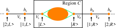
Figure 1: The schematic sketch of the electrode-junction-electrode system with semiperiodic one-dimensional electrodes.

The memory state $|M^{(m)}\rangle$ stems from the the second term on the r.h.s. of Eq. (16) and reads

$$|M^{(0)}\rangle=0,$$ (20)

while for $m\geq 1$ we have

$$|M^{(m)}\rangle = \delta^{2}\sum_{\alpha=L,R}|\alpha\rangle\sum_{k=0}^{m-1}\left[\langle\alpha|\psi_{C}^{(k+1)}\rangle+\langle\alpha|\psi_{C}^{(k)}\rangle\right]$$ (21)

$$\times \left[q_{\alpha}^{(m-k)}+q_{\alpha}^{(m-k-1)}\right].$$

The $q$-coefficients can be computed recursively according to

$$q_{\alpha}^{(0)}=\frac{-(1+i\delta h_{\alpha})+\sqrt{(1+i\delta h_{\alpha})^{2}+(2\delta V_{\alpha})^{2}}}{2\delta^{2}},$$ (22)

$$q_{\alpha}^{(1)}=\frac{1-i\delta h_{\alpha}-2\delta^{2}q_{\alpha}^{(0)}}{1+i\delta h_{\alpha}+2\delta^{2}q_{\alpha}^{(0)}}q_{\alpha}^{(0)},$$ (23)

and for $m\geq 2$

$$q_{\alpha}^{(m)} = \frac{q_{\alpha}^{(1)}q_{\alpha}^{(m-1)}}{q_{\alpha}^{(0)}}-\delta^{2}\frac{q_{\alpha}^{(0)}q_{\alpha}^{(m-2)}}{1+i\delta h_{\alpha}+2\delta^{2}q_{\alpha}^{(0)}}$$ (24)

$$- \delta^{2}\sum_{k=1}^{m-1}\frac{q_{\alpha}^{(k)}+2q_{\alpha}^{(k-1)}+q_{\alpha}^{(k-2)}}{1+i\delta h_{\alpha}+2\delta^{2}q_{\alpha}^{(0)}}q_{\alpha}^{(m-k)},$$

with the convention that $q_{\alpha}^{(m)}=0$ for negative $m$.

The source state $|S^{(m)}\rangle$ stems from the last term on the r.h.s. of Eq. (16) and reads

$$|S^{(m)}\rangle=-2i\delta\sum_{\alpha=L,R}\mbox{\boldmath$H$}_{C\alpha}\frac{({\bf 1}_{\alpha}-i\delta\mbox{\boldmath$H$}_{\alpha\alpha})^{m}}{({\bf 1}_{\alpha}+i\delta\mbox{\boldmath$H$}_{\alpha\alpha})^{m+1}}|\psi_{\alpha}(0)\rangle,$$ (25)

where ${\bf 1}_{\alpha}$ is the unit matrix in region $\alpha$. The source state depends on the initial wavefunction in the reservoirs. As we are interested in propagating eigenstates of $\mbox{\boldmath$H$}(0)$, $|\psi_{\alpha}(0)\rangle$ has the following general expression

$$|\psi_{\alpha}^{(0)}\rangle=A^{(+)}_{\alpha}|+p_{\alpha}\rangle+A^{(-)}_{\alpha}|-p_{\alpha}\rangle,$$ (26)

with

$$|p_{\alpha}\rangle=\sum_{j=1}^{\infty}e^{ip_{\alpha}j}|j;\alpha\rangle,$$ (27)

and the state $|j;\alpha\rangle$ where only the $j$-th site of reservoir $\alpha=L,\;R$ is occupied, see Fig. 1. For extendend states in region $\alpha$ the parameter $p_{\alpha}$ is real. For bound states or fully reflected states in region $\alpha$ the parameter $p_{\alpha}$ is imaginary and the amplitude ($A^{(+)}_{\alpha}$ or $A^{(-)}_{\alpha}$) of the growing exponential is zero. No matter if $p_{\alpha}$ is real or imaginary, one can prove that

$$\mbox{\boldmath$H$}_{C\alpha}\frac{({\bf 1}_{\alpha}-i\delta\mbox{\boldmath$H$}_{\alpha\alpha})^{m}}{({\bf 1}_{\alpha}+i\delta\mbox{\boldmath$H$}_{\alpha\alpha})^{m+1}}|p_{\alpha}\rangle=\zeta_{\alpha}^{(m)}|\alpha\rangle,$$ (28)

with

$$\zeta_{\alpha}^{(m)}=e^{ip_{\alpha}}V_{\alpha}\gamma_{\alpha}^{(m)}+i\delta\sum_{k=0}^{m}\gamma_{\alpha}^{(m-k)}\left[q_{\alpha}^{(k)}+q_{\alpha}^{(k-1)}\right],$$ (29)

and

$$\gamma_{\alpha}^{(m)}=\frac{(1-i\delta h_{\alpha}-2i\delta V_{\alpha}\cos p_{\alpha})^{m}}{(1+i\delta h_{\alpha}+2i\delta V_{\alpha}\cos p_{\alpha})^{m+1}}.$$ (30)

Finally, the effective Hamiltonian is given by

$$\mbox{\boldmath$H$}_{\rm eff}^{(m)}=\mbox{\boldmath$H$}_{CC}^{(m)}-i\delta\sum_{\alpha=L,R}q_{\alpha}^{(0)}|\alpha\rangle\langle\alpha|.$$ (31)

The above algorithm allows us to calculate the time evolution of any initial state whose wavefunction in the reservoirs has the form in Eq. (26). This is the case of both the contacting approach by Caroli and coworkers and the partition-free approach by Cini. In the former approach, the initial one-particle states are eigenstates of the isolated left and right reservoirs, meaning that

$$|\psi_{\alpha}^{(0)}\rangle=2\sum_{j=1}^{\infty}\sin(p_{\alpha}j)|j;\alpha\rangle=\frac{|+p_{\alpha}\rangle-|-p_{\alpha}\rangle}{i},$$ (32)

for $\alpha=L$ (or $\alpha=R$), zero for $\alpha=R$ (or $\alpha=L$), and zero in region $C$. In the latter approach the computation of the initial one-particle states is more involved. Here we have used a recently proposed general scheme based on the diagonalization of the imaginary part of the retarded Green’s function.ksarg.2005 This scheme may also be used for arbitrary, semiperiodic electrodes. In the special case of spatially uniform one-dimensional reservoirs one can, of course, always use the textbook procedure of matching the wavefunction at the interfaces.

Denoting with $|\psi_{s,C}(t)\rangle$ the evolution of the original eigenstate $|\psi_{s}(0)\rangle$ in the central region, we can calculate the time dependent occupation $\rho(j,t)$ of a state $|j\rangle$ in region $C$ according to

$$\rho(j,t)=\sum_{s}f(\varepsilon_{s})\left|\langle j|\psi_{s,C}(t)\rangle\right|^{2},$$ (33)

where $\varepsilon_{s}$ is the eigenvalue of $|\psi_{s}(0)\rangle$ and $f(\varepsilon)$ is the Fermi distribution function. Similarly, the total time-dependent current $I_{\alpha}(t)$ can be calculated from the time-derivative of the total number of particles in electrode $\alpha$ and reads

$$I_{\alpha}(t) = -2\sum_{s}f(\varepsilon_{s})\sum_{j\neq\alpha}$$ (34)

$$\times {\rm Im}\,\langle j|\psi_{s,C}(t)\rangle\langle\psi_{s,C}(t)|\alpha\rangle[\mbox{\boldmath$H$}_{CC}(t)]_{\alpha j},$$

where the sum is over all states $j$ of region $C$ except the state $|\alpha\rangle$.

We wish to conclude this Section with a discussion on the performance of our method and a comparison with Floquet-based approaches.

(i) The computational time $T_{\rm run}$ scales linearly with the number of states $N_{s}$ used to evaluate the sum in Eq. (33) or Eq. (34), and quadratically with the number of time steps $N_{t}$. In most cases transient effects disappear after few femtoseconds (few tens of atomic units). Using a time step of the order of $10^{-2}$ a.u. we can obtain a rather good estimate of $I_{\alpha,\rm dc}$ with $N_{t}\sim 10^{3}$ to $10^{4}$. Given a central regions with hundreds of states the real time algorithm can be of the same speed of or even faster than the Floquet algorithm of Appendix A.

(ii) The real-time algorithm can deal with arbitrary (periodic and non-periodic) drivings, and the computational time is independent of the specific time dependence of $\mbox{\boldmath$H$}_{CC}(t)$. Moreover, the algorithm is easily generalizedksarg.2005 to deal with spatially uniform bias potentials in the electrodes with arbitrary dependence on time such as, e.g., for an ac bias.

(iii) From the time-evolved states $|\psi_{s}(t)\rangle$ we have access to the total current $I_{\alpha}(t)$ at any time $t$, and not only to the long-time limit of the dc component of $I_{\alpha}(t)$. In particular, we can easily investigate transients and the full shape of $I_{\alpha}(t)$ for $t\rightarrow\infty$. In practice, this limit is achieved for a finite time $T_{\rm max}$ after which all transient phenomena have died out.

(iv) Another advantage of our method is the possibility of including electron-electron interactions via time-dependent density functional theory.rg.1984 Indeed, the external potential is local in both space and time provided the initial state is the ground state of the contacted system. Therefore, according to the Runge-Gross theorem,rg.1984 ; vl.1999 the interacting time-dependent density can be reproduced in a fictitious system of non-interacting electrons moving under the influence of an effective Kohn-Sham potential which is local in space and time. We observe that this is not the case in the contacting approach since the switching of the contacts makes the external potential non-local in space and hence the Runge-Gross theorem does not apply.

(v) Finally, we would like to stress that the Hamiltonian $\mbox{\boldmath$H$}_{CC}(t)$ enters in the algorithm only via the effective Hamiltonian $\mbox{\boldmath$H$}_{\rm eff}$ of Eq. (31), and has no restrictions. Thus, besides one-dimensional structures (like those considered in Section III) one can consider other geometries as well, like those of planar molecules, quantum rings, nanotubes, jellium slabs, etc.

III Numerical results

In this Section we illustrate the performance of the proposed scheme by presenting our results for one-dimensional continuos systems described by the time-dependent Hamiltonian

$$H(x,t)=-\frac{\nabla^{2}}{2}+U(x,t).$$ (35)

We discretize $H$ on a equidistant grid and use a three-point discretization for the kinetic term. Within this model we study various model systems highlighting different features in electron pumping.

III.1 Archimedean screw

As a first example of electron pumping we have calculated the time evolution of the density and total current for a single square barrier exposed to a travelling potential wave $U(x,t)=U_{1}\sin(qx-\omega_{0}t)$. The wave is spatially restricted to the explicitly treated device region which in our case also coincides with the static potential barrier. The barrier extends from $x=-8$ to $x=+8$ a.u. and its height is 0.5 a.u., see inset (b) in Fig 2. The system is unbiased, i.e., $U_{L}=U_{R}=0$, and the Fermi energy of the initial (ground) state is $\varepsilon_{\rm F}=0.3$ a.u.. For the numerical implementation we have chosen a lattice spacing $\Delta x=0.08$ a.u., and 200 $k$-points between 0 and $k_{\rm F}=\sqrt{2\varepsilon_{\rm F}}$ which amounts to the propagation of 400 states.

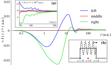
Figure 2: Time-dependent average current at the left and right interface and in the middle of region $C$ for pumping through a single square barrier by a travelling wave. The travelling potential wave is restricted to the propagation window $|x|<8$ a.u. and has the form $U(x,t)=U_{1}\sin(qx-\omega_{0}t)$ with amplitude $U_{1}=0.35$ a.u., wave number $q=1.6$ a.u. and frequency $\omega_{0}=0.2$ a.u.. Inset (a) is a magnification of the long-time behavior. The straight line corresponds to the value $I_{L,\rm dc}=7.63\cdot 10^{-4}$ a.u. of the average current calculated using the Floquet algorithm. Inset (b) displays the static potential barrier (solid line) and the superimposed right-moving travelling wave (dashed line).

In Fig. 2 we plot the time-dependent average current calculated according to

$$\langle I(t)\rangle = \theta(T_{0}-t)\frac{1}{t}\int_{0}^{t}{\rm d}\tau\,I(\tau)$$ (36)

$$+ \theta(t-T_{0})\frac{1}{T_{0}}\int_{t-T_{0}}^{t}{\rm d}\tau\,I(\tau),$$

with the period of the travelling wave $T_{0}=2\pi/\omega_{0}$. For the time propagation we have chosen a time step $2\delta=0.02$ a.u.. As expected $\langle I(t)\rangle$ converges to some steady value $I_{L,\rm dc}$ after a transient time of the order of $50\div 60$ a.u.. We have calculated the average current in three different points of region $C$ and verified that the steady value does not depend on the position. The dc limit $I_{L,\rm dc}$ can also be computed from the Floquet algorithm of Appendix A. Using $m_{\rm max}=15$ and $N_{\omega}=150$ energy points between 0 and $\varepsilon_{\rm F}$, we find $I_{L,\rm dc}=7.63\cdot 10^{-4}$ a.u., in very good agreement with the average current of the time propagated system, see inset (a) of Fig. 2.

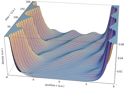
Figure 3: Time-dependent density in region $C$ as a function of position $x$ and time $t$. The range for $\rho(x,t)$ is between 0 and 0.06 a.u. for improved visibility of the pockets of density. All parameters are the same as for Fig. 2.

In Fig. 3 we plot the time-dependent density $\rho(x,t)$ in the device region as a function of both position $x$ and time $t$. The density exhibits local maxima in the potential minima and is transported in pockets by the wave. From Fig. 3 it is also evident that the height of the pockets is not uniform over the system, and reaches its maximum around $x=0$. We also notice that the particle current flows in the same direction as the driving wave. The pumping mechanism in this example resembles pumping of water with the Archimedean screw.

III.2 Pumping through a semiconductor nanostructure

The second example was motivated by a recent experiment on pumping through a carbon nanotube.lbtsajwc.2005 The arrangement has been suggested by Talyanskii et al.tnsl.2001 and is as follows. A semiconducting nanotube lying on a quartz substrate is placed between two metallic contacts. A transducer generates an acoustic wave on the surface of the piezoelectric crystal. The crystal responds by generating an electrostatic potential wave which acts like our travelling wave on the electrons in the nanotube. The direction of the pumping current is found to depend on the applied gate voltage. A pumping current flowing in the direction opposite to the propagation direction of the travelling wave has been interpreted in a stationary picture as a predominant hole tunneling over electron tunneling. To reproduce such an inversion in the current flow we have modelled the nanotube with a periodic static corrugation $U_{0}(x)=U_{C}(1+\cos(kx))$ in region $C$, with $U_{C}=0.5$ a.u. and $k=10\pi/6\sim 5.2$ a.u. (see inset in Fig 4). For a travelling wave $U(x,t)=U_{1}\sin(qx-\omega_{0}t)$, with $U_{1}=0.5$ a.u., $\omega_{0}=0.8$ a.u., and $q=0.6$ a.u., we have found that the minimum current occurs at $\varepsilon_{\rm F}=3.0$ a.u.. All parameters in this example have been chosen to better illustrate and discuss the effect of the current inversion. The present Section is not intended to give a realistic description of some specific experiment.

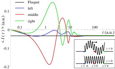
Figure 4: Time-dependent average current at the left and right interface and in the middle of region $C$ for pumping through a device region which extends from $x=-6$ to $x=6$ a.u.. A travelling wave $U(x,t)=U_{1}\sin(qx-\omega_{0}t)$ with $U_{1}=0.5$ a.u., $\omega_{0}=0.8$ a.u., and $q=0.6$ a.u., is superimposed to the static potential $U_{0}(x)=U_{C}(1+\cos(kx))$ with $U_{C}=0.5$ a.u. and $k=10\pi/6\sim 5.2$ a.u., and the all system is unbiased, see inset. The straight line corresponds to the value of the average current as obtained from the Floquet algorithm which yields $I_{L,\rm dc}=3.26\cdot 10^{-2}$ a.u..

In Fig. 4 we plot the time-dependent average current [see Eq. (36)] in three different points of the device region. For the numerical propagation we have used a lattice spacing $\Delta x=0.06$ a.u., a time step $2\delta=0.02$ a.u., and $400$ $k$-points between $0$ and $k_{\rm F}=\sqrt{2\varepsilon_{\rm F}}$. The system responds to a right-moving travelling wave by generating a net current flowing to the left. Again we observe that the transient time is of the order of few tens of atomic units, and that the steady value is independent of the position. As in the previous example, we used the Floquet algorithm of Appendix A for benchmarking our real-time propagation algorithm. Due to the high Fermi energy the calculation was carried out with $m_{\rm max}=15$ and $N_{\omega}=400$ energy points between 0 and $\varepsilon_{\rm F}$. The result $I_{L,\rm dc}=3.26\cdot 10^{-2}$ a.u. is displayed in Fig. 4 with a straight line and is in extremely good agreement with the long-time limit of the average current obtained from direct propagation in time.

To understand how the electron fluid moves when the direction of the current is opposite to that of the driving potential wave, we have studied the dynamical flow pattern of the density. We emphasize that such a study would have been rather complicated in Floquet-based approaches. The latter are often used as “black boxes”, and one needs to resort to limiting cases, like, e.g., the adiabatic picture, the high frequency limit, the theory of linear response, etc., for a qualitative understanding.

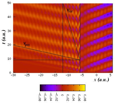
Figure 5: Contour plot of the excess density $\Delta\rho(x,t)$ in the device region ($x$ between -6 and 6 a.u.) and in a portion of the left reservoir ($x$ between -30 and -6 a.u.). Due to the large oscillations of the excess density in the device region, $\Delta\rho(x,t)$ has been scaled down by a factor of 10 for $|x|<6$ a.u.. We also draw straight lines to show a pocket trajectory and the trajectory of a superimposed oscillation. All parameters are the same as for Fig. 4.

In Fig. 5 we display a contour plot of the excess density $\Delta\rho(x,t)=\rho(x,t)-\rho(x,0)$ in an extended region which includes the device region and a portion of the left reservoir. In the device region we clearly see pockets that are dragged by the travelling wave and are moving to the right. However, every pocket with a slightly positive $\Delta\rho$ is followed by a pocket with a noticeably negative $\Delta\rho$, and the net excess density is negative. On the other hand, in the left reservoir only pockets with a positive $\Delta\rho$ exist and they move to the left. We conclude that the driving produces right-moving “bubbles” in the device region and that to each bubble corresponds a more dense region of fluid moving to the left. One can estimate the speed $v_{\rm poc}$ of the travelling pockets from the slope of the patterns at constant density and find $v_{\rm poc}\sim\omega_{0}/q\sim 1.33$ a.u., as expected. We also notice superimposed density oscillations on each pocket. These oscillations have the same spatial period of the static corrugation in the device region, and move in the same direction of the pockets at a constant speed $v_{\rm osc}\sim\omega_{0}/k\sim 0.15$ a.u..

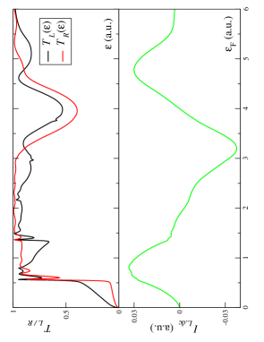
Figure 6: dc component of pump current $I_{L,\rm dc}$ and left/right transmission probabilities $T_{L/R}$ as function of the Fermi energy. The curves have been obtained using the Flocquet algorithm of Appendix A with $m_{\rm max}=15$ and $N_{\omega}=800$ energy points between 0 and $\varepsilon_{\rm F}=6$ a.u..

In Fig. 6 we illustrate how the pumped current in this model depends on the Fermi level. For Fermi energies comparable to the amplitude of the corrugated potential in the device region the pumping current is always positive, i.e., follows the propagation of the perturbed wave. However, there are striking effects that are more or less independent of the strength of the perurbation: the pumping current reaches a maximum positive value at $\varepsilon_{\rm F}\sim\omega_{0}=0.8$ a.u., then decreases with increasing Fermi energy (with the turning point to negative values just below $\varepsilon_{\rm F}=2$ a.u.) and reaches a minimum (negative) value above $\varepsilon_{\rm F}=3$ a.u.. To rationalise this behavior we have calculated the total transmission probabilities $T_{\alpha}=\sum_{m}T_{m,\alpha}$, $\alpha=L,R$, for left- and right-going electrons [see Eqs. (11, 12)]. As one can see from Fig. 6, both $T_{L}$ and $T_{R}$ remain quite small for Fermi energies below $\Delta\sim 0.54$ a.u., which roughly corresponds to the bottom of the lowest band of the periodic structure of the device. In this energy window transport is dominated by tunneling and the pumping current follows the travelling wave ($T_{L}>T_{R}$) similar to the case of the Archimedean screw, see Section III.1. For $\varepsilon_{\rm F}>\Delta$ we enter the region of resonant transport (the energy of the lowest band) and $T_{L}$, $T_{R}$ sharply increase. We observe that for $\varepsilon_{\rm F}<\omega_{0}=0.8$ a.u. both $T_{L}$ and $T_{R}$ have a structure similar to the total transmission function of the static case. For $\omega_{0}<\varepsilon_{\rm F}<\omega_{0}+\Delta$, however, $T_{L}$ decreases significantly while $T_{R}$ remains fairly constant around 1. We interpret this in the following way. The probability of the right-going electrons of emitting a photon of frequency $\omega_{0}$ (and therefore reducing their energy) is larger than for the left-going electrons. Loosing this energy, the transmission $T_{L}$ resembles the static transmission function for energy $\varepsilon_{\rm F}-\omega_{0}$ which has a much lower value. The asymmetry between left- and right-going states can easily be understood by realizing that the pump wave introduces a preferential direction in the problem. As further evidence to support this interpretation we note that for $\varepsilon_{\rm F}=\omega_{0}+\Delta$ the transmission function $T_{L}$ increases rapidly as for $\varepsilon_{\rm F}=\Delta$. This can be viewed as a replica of the static transmission function shifted by one quantum of energy $\omega_{0}$. Throughout the energy window of the lowest band, $T_{L}$ remains lower than $T_{R}$. As a consequence the pumping current decreases monotonically. This behaviour is reversed when the Fermi energy hits the top of the lowest band, around $3.4$ a.u.. In the gap (of about $2U_{C}=1$ a.u.) both $T_{L}$ and $T_{R}$ drop and transport is dominated by tunneling again. In this region $T_{L}>T_{R}$ and the pumping current increases.

The present model gives positive and negative pumping current as a function of the Fermi energy and provides a simple physical interpretation of the effect of current inversion. Our picture, however, is somewhat different from the one given by Leek et al.. lbtsajwc.2005 Indeed, in their explanation the sign of the pumping current is independent of the frequency $\omega_{0}$ of the travelling wave. On the other hand, in our case, if the frequency exceeds the width of the lowest band, the right-going electrons cannot emit a photon and current inversion is not guaranteed anymore.

III.3 Transients effects

As a last example we study electron pumping in quantum wells. We will show the presence of long-lived superimposed oscillations whose frequency is generally not commensurable with the driving frequency. The quantum well is modelled with a static potential $U_{0}(x)=-1.4$ a.u. for $|x|<1.2$ a.u. and zero otherwise. Initially the system is in the ground state with Fermi energy $\varepsilon_{\rm F}=0.1$ a.u.. The unperturbed Hamiltonian has two bound-state eigensolutions with energy $\varepsilon^{0}_{b,1}=-1.035$ a.u. and $\varepsilon^{0}_{b,2}=-0.156$ a.u.. The ground-state Slater determinant contains all extended states with energy between 0 and $\varepsilon_{\rm F}$ and two localized states with negative energy. At positive times a constant bias $U_{R}=0.1$ a.u. is applied on the right lead and a travelling wave $U(x,t)=U_{1}\sin(qx-\omega_{0}t)$, with $q=0.5$ a.u. and $\omega_{0}=0.5$ a.u., is switched on in the quantum well. In the numerical simulations we set the propagation window between $x=-1.2$ and $x=1.2$ a.u. (which coincides with the static potential well) and choose a lattice spacing $\Delta x=0.024$ a.u.. The occupied part of the continuum spectrum is discretized with 100 $k$-points between 0 and $k_{\rm F}=\sqrt{2\varepsilon_{\rm F}}$.

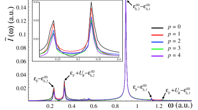
Figure 7: Modulus of the discrete Fourier transform of the current for zero driving and $U_{R}=0.1$ a.u.. The inset shows a magnification of the region with bound-continuum transitions. Different curves correspond to different time intervals.

Let us first consider the biased system with no driving, i.e., $U_{1}=0$. We propagate the (non-interacting) many-body state from $t=0$ to $t=1400$ a.u. using a time step $2\delta=0.05$ a.u., and calculate the current $I(t)$ at the center of the quantum well. As in the examples of Sections III.1 and III.2, one observes a first transient behavior which lasts for few tens of atomic units. However, after this first normal transient a second transient regime sets in. In Fig. 7 we plot the modulus of the discrete Fourier transform of the current

$$\tilde{I}(\omega_{k})=2\delta\sum_{n=n_{p}}^{n_{p}+N_{0}}I(2n\delta)e^{-i\omega_{k}n\delta},\quad\omega_{k}=\frac{2\pi k}{N_{0}\delta}$$ (37)

for $n_{p}=(4+2p)\cdot 10^{3}$, $p=0,1,2,3,4$, and $N_{0}=16\cdot 10^{3}$ (corresponding to the time intervals $t\in(t_{p},t_{p}+T_{0})$ with $t_{p}=(2+p)\times 100$ a.u. and $T_{0}=800$ a.u.). Besides the zero-frequency peak (not shown) due to the non vanishing dc current, the structure of $\tilde{I}(\omega)$ has five more peaks. Below we discuss the physical origin of these extra peaks and show that they are related to different kinds of internal transitions.

We first observe that the biased system has two bound states with energy $\varepsilon_{b,1}^{\infty}=-1.032$ a.u. and $\varepsilon_{b,2}^{\infty}=-0.133$ a.u. (slightly different from the bound-state energies of the unbiased system). The first and the last two peaks occur at the same frequency of the bound-continuum transitions $\varepsilon_{b,i}^{\infty}\rightarrow\varepsilon_{\rm F}$, and $\varepsilon_{b,i}^{\infty}\rightarrow\varepsilon_{\rm F}+U_{R}$, with $i=1,2$. These sharp structures (mathematically stemming from the discontinuity of the zero-temperature Fermi distribution function) give rise to long-lived oscillations of the total current and density. Such an oscillatory transient regime dies off slowly as $1/t$. The power-low behavior can also be seen in the inset of Fig. 7, where a magnification of the region with transitions from the weakly bound electron to the two continua is displayed. Denoting with $R_{p}$ the product between the height of the second peak and the propagation time $t_{p}+T_{0}$ we have found $R_{2}=26.305$ a.u., $R_{3}=26.307$ a.u., and $R_{4}=26.328$ a.u., which is in fairly good agreement with the expected $1/t$ behavior. Therefore, the hight of the peaks decreases with increasing $t_{p}$ and approaches zero in the limit $t_{p}\rightarrow\infty$. On the contrary, the sharp peak at $\omega=\varepsilon_{b,1}^{\infty}-\varepsilon_{b,2}^{\infty}$ (bound-bound transition) remains unchanged with increasing $t_{p}$. The oscillations of the bound-bound transition do not die off, in agreement with the findings of Refs. ds.2006, ; s.2006, . We emphasize that these latter oscillations are an intrinsic property of the biased system and have nothing to do with external drivings.

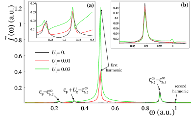
Figure 8: Modulus of the discrete Fourier transform of the current for the biased quantum well ($U_{R}=0.1$ a.u.) perturbed by the travelling wave $U(x,t)=U_{1}\sin(qx-\omega t)$, with $q=0.5$ a.u. and $\omega=0.5$ a.u.. Three different amplitudes $U_{1}=0.00,\,0.01,\,0.03$ a.u. are considered. Inset (a) displays a magnification of the region with bound-continuum transitions. Inset (b) shows a magnification of the region with the bound-bound transition and the second-harmonic peak.

Having discussed the behavior of the system which is biased but not driven, we now study transient regimes in the biased and driven system, i.e., $U_{1}\neq 0$. Using the same numerical parameters as in the previous example we evolve the (non-interacting) many-body state from $t=0$ to $t=1200$ a.u. with a time step $2\delta=0.05$ a.u.. In Fig. 8 we plot the discrete Fourier transform of the current calculated in the middle of the quantum well for different amplitudes of the travelling wave $U_{1}=0.00,\,0.01,\,0.03$ a.u.. The time interval used to evaluate $\tilde{I}(\omega)$ is from $t=200$ a.u. to $t=1200$ a.u.. As expected, $\tilde{I}(\omega)$ has a well pronounced peak at the driving frequency (first harmonic). Increasing the amplitude of the driving field the height of the first-harmonic peak increases and higher-order harmonic peaks become visible (breakdown of linear response theory). This is clearly shown in inset (b) where the second-harmonic peak is visible for $U_{1}=0.03$ a.u. but not for $U_{1}=0.01$ a.u.. The structure of $\tilde{I}(\omega)$ has also other peaks at frequencies which are not commensurable with the driving frequency. Such peaks are due to the presence of bound states in the biased-only system. In inset (a) we show a magnification of the region with bound-continuum transitions. The driving field broadens the peak-structure, thus speeding up the power-law transient regime. The shape of the bound-bound transition is displayed in inset (b). The height of the peak decreases with increasing amplitudes and the transition changes from an infinitely long-lived excitation to an excitation with a finite life time. Let $m_{s}$ be the smallest integer for which $m_{s}\omega_{0}>\max(|\varepsilon_{b,1}^{\infty}|,|\varepsilon_{b,2}^{\infty}|)$; for small amplitudes the life time is proportional to $(1/U_{1}^{2})^{m_{s}}$ according to the following reasoning. The retarded Green’s function in region $C$ can be written in terms of the embedding self-energy of Eq. (4) and the Floquet self-energy $\mbox{\boldmath$\Sigma$}^{\rm R}_{\rm ac}$ of Eq. (55). The Floquet self-energy generates replica of the continuous spectrum which are shifted by multiple integers of $\omega_{0}$ and contributes to the imaginary part of the Green’s function, $\mbox{\boldmath$G$}^{\rm R}$. The leading-order contribution of the $m$-th replica to ${\rm Im}\,\mbox{\boldmath$G$}^{\rm R}$ scales like $(U_{1}^{2})^{m}$. Therefore, bound-state simple poles of $\mbox{\boldmath$G$}^{\rm R}$ get embedded in the continuum spectrum of some of the replica and aquire an imaginary part proportional to $(U_{1}^{2})^{m}$, with $m$ the order of the replica. The leading-order contribution to the life-time of the bound-bound excitation is then proportional to $(1/U_{1}^{2})^{m_{s}}$.

In conclusion, we have shown that the biased and driven quantum well has a very rich transient structure. This is due to the presence of bound states which can substantially delay the development of the Floquet regime.

IV Conclusions and outlooks

Time-dependent gate voltages can be used to generate a net current between unbiased electrodes in nanoscale junctions. Most works focus on periodic drivings for which Floquet-based approaches provide a powerful machinery to investigate the long-time behavior of the system. Combining Floquet theory with nonequilibrium Green’s functions techniques we obtained a general formula for the average current of monochromatically driven systems in terms of inelastic transmission probabilities. The case of polychromatic drivings, which has received scarce attention so far, is analytically more complicated and computationally rather costly.

In this work we proposed an alternative approach which can deal with monochromatic, polychromatic and nonperiodic drivings. The computational cost is independent of the particular time dependence of the driving potential. As an extra bonus we can investigate how the transient behavior depends on the initial state and on the details of the switching process. The basic idea is to calculate the time-dependent density and current from the time-evolved (non-interacting) many-particle state. This amounts to solving a single-particle Schrödinger equation for each occupied eigenstate of the unperturbed system. We have given full implementation details of the time-propagation algorithm and discussed its performance. The generalization to two- or three-dimensional reservoirs can be worked out following the general lines of Ref. ksarg.2005, and its implementation is in progress.

We illustrated our scheme in one-dimensional structures. First we studied pumping through a single barrier, and showed that the electrons are dragged by the travelling wave and move in pockets. Second we studied pumping in semiconducting structures, and investigated the phenomenon of current inversion. In both examples the Floquet algorithm of Appendix A is used for benchmarking the long-time limit of the real-time simulations and we have found an excellent agreement between the two approaches. Finally, we considered pumping through a quantum well connected to biased reservoirs. The aim of this latter example is to show the existence of a long-lived transient regime in rather common physical systems. The transient oscillations are explained in terms of bound-bound transitions and bound-continuum transitions. These oscillations usually have frequencies which are not commensurable with the driving frequency and are therefore not described by the initial Floquet assumption.

The present work opens the path towards systematic studies of nanoscale devices as it is not restricted to linear response theory and can cope with general time-dependent as well as spatial perturbations. Our approach can also be extended in a natural way to describe more complicated physical systems. The effects of electron correlation may be included within the framework of time-dependent density functional theoryksarg.2005 by using present exchange-correlation density functionals as well as orbital dependent ones. Second, the scheme can be upgraded to cope with three-dimensional reservoirs. This is computationally more demanding but clearly will pay back in our understanding of non-equilibrium dynamical phenomena in nanoconstrictions.

Highlighting different physical phenomena, our idea of real-time evolution of open quantum systems may also be used to address questions such as time-dependent spin transport, current fluctuations and shot noise, optimal control of devices for quantum information processing, rcwrg.2006 the role of superconducting leads, heat transport, etc.. In particular, the design of fast, integrated, optoelectronic nanodevices clearly requires the proper description of dynamical effects (relaxation, decoherence, etc.) on a microscopic level. Problems related to current induced heating and electromigration should also be addressed,vsa.2006 ; dvp.2000 ; hbf.2004 ; mrt.2006 and one might need to go beyond the classical treatment of the ionic motion as it fails in describing Joule heating.hbftm.2004 ; hbfts.2004 ; bhst.2005 The present work is a small step towards those ambitious goals, adding the physics of time-dependent phenomena to the world of steady-state effects in quantum transport.

Appendix A Current formula

The dc kernel $\mbox{\boldmath$Q$}_{\alpha,\rm dc}$ in Eq. (7) is given by the sum of two terms, both containing an integral over energy $\omega$. Consequently, also the total dc current can be expressed as the sum of two terms. From Eq. (2) it is straightforward to obtain

$$I_{\alpha,\rm dc}=I_{\alpha}^{(1)}+I_{\alpha}^{(2)},$$ (38)

with

$$I_{\alpha}^{(1)}=-2\int\frac{{\rm d}\omega}{2\pi}f_{\alpha}(\omega)\,{\rm Im}\,{\rm Tr}\left[\mbox{\boldmath$\Gamma$}_{\alpha}(\omega)\mbox{\boldmath$G$}_{0}(\omega)\right],$$ (39)

and

$$I_{\alpha}^{(2)}=-\int\frac{{\rm d}\omega}{2\pi}\sum_{\beta}f_{\beta}(\omega)\sum_{m}\quad\quad\quad\quad\quad\quad\quad\;\,$$

$$\times{\rm Tr}\left[\mbox{\boldmath$G$}_{m}(\omega)\mbox{\boldmath$\Gamma$}_{\beta}(\omega)\mbox{\boldmath$G$}^{{\dagger}}_{m}(\omega)\mbox{\boldmath$\Gamma$}_{\alpha}(\omega-m\omega_{0})\right].$$ (40)

Let us focus on the coeffiecients $\mbox{\boldmath$G$}_{m}$ and derive a recursive scheme to calculate them. We write the Hamiltonian $\mbox{\boldmath$H$}_{CC}(t)$ as the sum of a static, $\mbox{\boldmath$H$}_{CC}^{0}$, and periodic, $\mbox{\boldmath$U$}_{CC}(t)$, term and expand the latter in Fourier modes

$$\mbox{\boldmath$U$}_{CC}(t)=\sum_{n}\mbox{\boldmath$U$}_{n}e^{in\omega_{0}t},\quad\quad\mbox{\boldmath$U$}_{n}=\mbox{\boldmath$U$}^{{\dagger}}_{-n}.$$ (41)

We also define the Green’s function $g$ as the projection onto region $C$ of the Green’s function of the system which is biased but not driven, i.e., $\mbox{\boldmath$U$}_{CC}(t)=0$. The Green’s function $g$ depends only on the difference between its time arguments and can be expanded as follows

$$\mbox{\boldmath$g$}^{\rm R}(t;t^{\prime})=\sum_{m}\int\frac{{\rm d}\omega}{2\pi}\mbox{\boldmath$g$}^{\rm R}_{m}(\omega)e^{-i\omega(t-t^{\prime})+im\omega_{0}t^{\prime}},$$ (42)

where the only non-vanishing coefficient of the expansion is $\mbox{\boldmath$g$}^{\rm R}_{0}(\omega)$ and reads

$$\mbox{\boldmath$g$}^{\rm R}_{0}(\omega)=\frac{1}{\omega{\bf 1}_{C}-\mbox{\boldmath$H$}_{CC}^{0}-\mbox{\boldmath$\Sigma$}^{\rm R}(\omega)},$$ (43)

with ${\bf 1}_{C}$ the unit matrix in region $C$ and $\mbox{\boldmath$\Sigma$}^{\rm R}$ the retarded embedding self-energy of Eq. (4). Inserting the above expansions into the Dyson equation

$$\mbox{\boldmath$G$}^{\rm R}(t;t^{\prime})=\mbox{\boldmath$g$}^{\rm R}(t;t^{\prime})+\int{\rm d}\bar{t}\;\mbox{\boldmath$g$}^{\rm R}(t;\bar{t})\mbox{\boldmath$U$}_{CC}(\bar{t})\mbox{\boldmath$G$}^{\rm R}(\bar{t};t),$$ (44)

we find a set of linear equations for the coefficients $\mbox{\boldmath$G$}_{m}$

$$\mbox{\boldmath$G$}_{m}(\omega)=\delta_{m,0}\mbox{\boldmath$g$}_{m}(\omega)+\mbox{\boldmath$g$}_{m}(\omega)\sum_{n}\mbox{\boldmath$U$}_{n}\mbox{\boldmath$G$}_{m-n}(\omega),$$ (45)

where we have used the short-hand notation $\mbox{\boldmath$g$}_{m}(\omega)=\mbox{\boldmath$g$}^{\rm R}_{0}(\omega-m\omega_{0})$ (the $\mbox{\boldmath$g$}_{m}$ should not to be confused with the expansion coefficient $\mbox{\boldmath$g$}_{m}^{\rm R}$ of Eq. (42); the latter is zero for all $m\neq 0$). For arbitrary periodic drivings the solution of Eq. (45) is computationally very hard. In the following we specialize to the monochromatic case and describe a feasible numerical scheme to calculate the $\mbox{\boldmath$G$}_{m}$’s.

For monochromatic drivings, $\mbox{\boldmath$U$}_{n}=\delta_{n,1}\mbox{\boldmath$U$}_{+}+\delta_{n,-1}\mbox{\boldmath$U$}_{-}$, the algebraic system in Eq. (45) simplifies to (understanding the quantities as function of $\omega$)

$$\mbox{\boldmath$G$}_{m}=\mbox{\boldmath$g$}_{m}\left[\delta_{m,0}+\mbox{\boldmath$U$}_{+}\mbox{\boldmath$G$}_{m-1}+\mbox{\boldmath$U$}_{-}\mbox{\boldmath$G$}_{m+1}\right],$$ (46)

which is a tridiagonal system. In matrix form Eq. (46) reads

$$\left[\begin{array}[]{cccc|c|cccc}&&&&\vdots&&&&\\ &&\underline{\mbox{\boldmath$M$}}^{(-)}&&0&&\underline{{\bf 0}}&&\\ &&&&0&&&&\\ &&&&-\mbox{\boldmath$g$}_{-1}\mbox{\boldmath$U$}_{-}&&&&\\ \hline\cr\ldots&0&0&-\mbox{\boldmath$g$}_{0}\mbox{\boldmath$U$}_{+}&{\bf 1}_{C}&-\mbox{\boldmath$g$}_{0}\mbox{\boldmath$U$}_{-}&0&0&\ldots\\ \hline\cr&&&&-\mbox{\boldmath$g$}_{1}\mbox{\boldmath$U$}_{+}&&&&\\ &&&&0&&&&\\ &&\underline{{\bf 0}}&&0&&\underline{\mbox{\boldmath$M$}}^{(+)}&&\\ &&&&\vdots&&&&\\ \end{array}\right]\left[\begin{array}[]{c}\vdots\\ \mbox{\boldmath$G$}_{-3}\\ \mbox{\boldmath$G$}_{-2}\\ \mbox{\boldmath$G$}_{-1}\\ \hline\cr\mbox{\boldmath$G$}_{0}\\ \hline\cr\mbox{\boldmath$G$}_{1}\\ \mbox{\boldmath$G$}_{2}\\ \mbox{\boldmath$G$}_{3}\\ \vdots\end{array}\right]=\left[\begin{array}[]{c}\vdots\\ 0\\ 0\\ 0\\ \hline\cr\mbox{\boldmath$g$}_{0}\\ \hline\cr 0\\ 0\\ 0\\ \vdots\end{array}\right]$$ (47)

where $\underline{{\bf 0}}$ is the null matrix and the matrices $\mbox{\boldmath$M$}^{(\pm)}$ read

$$\underline{\mbox{\boldmath$M$}}^{(-)}=\left[\begin{array}[]{ccccc}&\ddots&\ddots&0&0\\ \ldots&-\mbox{\boldmath$g$}_{-3}\mbox{\boldmath$U$}_{+}&{\bf 1}_{C}&-\mbox{\boldmath$g$}_{-3}\mbox{\boldmath$U$}_{-}&0\\ \ldots&0&-\mbox{\boldmath$g$}_{-2}\mbox{\boldmath$U$}_{+}&{\bf 1}_{C}&-\mbox{\boldmath$g$}_{-2}\mbox{\boldmath$U$}_{-}\\ \ldots&0&0&-\mbox{\boldmath$g$}_{-1}\mbox{\boldmath$U$}_{+}&{\bf 1}_{C}\end{array}\right],$$ (48)

$$\underline{\mbox{\boldmath$M$}}^{(+)}=\left[\begin{array}[]{ccccc}{\bf 1}_{C}&-\mbox{\boldmath$g$}_{1}\mbox{\boldmath$U$}_{-}&0&0&\ldots\\ -\mbox{\boldmath$g$}_{2}\mbox{\boldmath$U$}_{+}&{\bf 1}_{C}&-\mbox{\boldmath$g$}_{2}\mbox{\boldmath$U$}_{-}&0&\ldots\\ 0&-\mbox{\boldmath$g$}_{3}\mbox{\boldmath$U$}_{+}&{\bf 1}_{C}&-\mbox{\boldmath$g$}_{3}\mbox{\boldmath$U$}_{-}&\ldots\\ 0&0&\quad\quad\quad\ddots&\quad\quad\quad\quad\ddots&\end{array}\right].$$ (49)

Let $\mbox{\boldmath$M$}^{-1}_{-}$, $\mbox{\boldmath$M$}^{-1}_{+}$ be the bottom-right block of the inverse of $\underline{\mbox{\boldmath$M$}}^{(-)}$ and the top-left block of the inverse of $\underline{\mbox{\boldmath$M$}}^{(+)}$ respectively. The coefficient $\mbox{\boldmath$G$}_{\pm 1}$ can be expressed in terms of $\mbox{\boldmath$M$}^{-1}_{\pm}$ according to

$$\mbox{\boldmath$G$}_{\pm 1}=\mbox{\boldmath$M$}^{-1}_{\pm}\mbox{\boldmath$g$}_{\pm 1}\mbox{\boldmath$U$}_{\pm}\mbox{\boldmath$G$}_{0}.$$ (50)

Substituting this result into Eq. (46) with $m=0$, one obtains a closed equation for $\mbox{\boldmath$G$}_{0}$

$$\mbox{\boldmath$G$}_{0}=\mbox{\boldmath$g$}_{0}+\mbox{\boldmath$g$}_{0}\sum_{\pm}\mbox{\boldmath$U$}_{\mp}\mbox{\boldmath$M$}^{-1}_{\pm}\mbox{\boldmath$g$}_{\pm 1}\mbox{\boldmath$U$}_{\pm}\mbox{\boldmath$G$}_{0}.$$ (51)

Exploiting the tridiagonal block-structure of $\underline{\mbox{\boldmath$M$}}^{(\pm)}$ we can express the matrices $\mbox{\boldmath$M$}^{-1}_{\pm}$ as a continued matrix fraction

$$\mbox{\boldmath$M$}^{-1}_{\pm}=\frac{{\bf 1}_{C}}{{\bf 1}_{C}-\mbox{\boldmath$g$}_{\pm 1}\mbox{\boldmath$U$}_{\mp}\frac{\mbox{${\bf 1}_{C}$}}{\mbox{${\bf 1}_{C}-\mbox{\boldmath$g$}_{\pm 2}\mbox{\boldmath$U$}_{\mp}$}\frac{\mbox{${\bf 1}_{C}$}}{\quad\ddots}\mbox{$\mbox{\boldmath$g$}_{\pm 3}\mbox{\boldmath$U$}_{\pm}$}}\mbox{\boldmath$g$}_{\pm 2}\mbox{\boldmath$U$}_{\pm}}=\frac{{\bf 1}_{C}}{\mbox{\boldmath$g$}_{\pm 1}^{-1}-\mbox{\boldmath$U$}_{\mp}\frac{\mbox{${\bf 1}_{C}$}}{\mbox{$\mbox{\boldmath$g$}_{\pm 2}^{-1}-\mbox{\boldmath$U$}_{\mp}$}\frac{\mbox{${\bf 1}_{C}$}}{\quad\ddots}\mbox{$\mbox{\boldmath$U$}_{\pm}$}}\mbox{\boldmath$U$}_{\pm}}\mbox{\boldmath$g$}_{\pm 1}^{-1},$$ (52)

which is equivalent to solving the following recursive relations (remaking explicit the dependence on $\omega$)

$$\mbox{\boldmath$M$}_{\pm}^{-1}(\omega)=\mbox{\boldmath$H$}_{\pm,1}^{-1}(\omega)\mbox{\boldmath$g$}_{\pm 1}^{-1}(\omega).$$ (53)

and

$$\mbox{\boldmath$H$}_{\pm,m}^{-1}(\omega)=\frac{{\bf 1}_{C}}{\mbox{\boldmath$g$}^{-1}_{\pm m}(\omega)-\mbox{\boldmath$U$}_{\mp}\,\mbox{\boldmath$H$}^{-1}_{\pm,m+1}(\omega)\,\mbox{\boldmath$U$}_{\pm}}=\frac{{\bf 1}_{C}}{\left(\omega\mp m\omega_{0}\right){\bf 1}_{C}-\mbox{\boldmath$H$}^{0}_{CC}-\mbox{\boldmath$\Sigma$}^{\rm R}(\omega\mp m\omega_{0})-\mbox{\boldmath$U$}_{\mp}\,\mbox{\boldmath$H$}^{-1}_{\pm,m+1}(\omega)\,\mbox{\boldmath$U$}_{\pm}}.$$ (54)

Introducing the ac self-energy,

$$\mbox{\boldmath$\Sigma$}^{\rm R}_{\rm ac}(\omega)=\sum_{\pm}\mbox{\boldmath$U$}_{\mp}\,\mbox{\boldmath$H$}^{-1}_{\pm,1}(\omega)\,\mbox{\boldmath$U$}_{\pm},$$ (55)

which accounts for the interaction between the electrons and the ac driving field, we can rewrite the solution for $\mbox{\boldmath$G$}_{0}$ in Eq. (51) as

$$\mbox{\boldmath$G$}_{0}^{-1}(\omega)=\mbox{\boldmath$g$}_{0}^{-1}(\omega)-\mbox{\boldmath$\Sigma$}^{\rm R}_{\rm ac}(\omega)=\omega{\bf 1}_{C}-\mbox{\boldmath$H$}_{CC}^{0}-\mbox{\boldmath$\Sigma$}^{\rm R}(\omega)-\mbox{\boldmath$\Sigma$}^{\rm R}_{\rm ac}(\omega).$$ (56)

In our implementation we have solved the above recursive relations by truncating the hierarchy. For some $m=m_{\rm max}$ we set $\mbox{\boldmath$H$}_{\pm,m_{\rm max}}(\omega)=\mbox{\boldmath$g$}^{-1}_{\pm m_{\rm max}}(\omega)$, and calculate all the $\mbox{\boldmath$H$}_{\pm,m}(\omega)$ with $m<m_{\rm max}$ according to Eq. (54). The convergence of the result can be tested by increasing $m_{\rm max}$. Typically, the smaller $\omega_{0}$ the larger one has to choose $m_{\rm max}$ to achieve convergence. Once the matrix $\mbox{\boldmath$G$}_{0}$ has been calculated, the matrices $\mbox{\boldmath$G$}_{m}$ with $m\neq 0$ are easily obtained from

$$\mbox{\boldmath$G$}_{\pm m}(\omega)=\mbox{\boldmath$H$}^{-1}_{\pm,m}(\omega)\mbox{\boldmath$U$}_{\pm}\mbox{\boldmath$G$}_{\pm(m-1)}(\omega),\quad m>0.$$ (57)

Having explicit equations for the $\mbox{\boldmath$G$}_{m}$’s, we now show how to express the total dc current in terms of inelastic transmission probabilities. To calculate the contribution $I_{\alpha}^{(1)}$ in Eq. (39) we need to evaluate the imaginary part of ${\rm Tr}\left[\mbox{\boldmath$\Gamma$}_{\alpha}\mbox{\boldmath$G$}_{0}\right]$. Using the identity

$$\mbox{\boldmath$G$}_{0}-\mbox{\boldmath$G$}_{0}^{{\dagger}}=\mbox{\boldmath$G$}_{0}^{{\dagger}}\left(\mbox{\boldmath$\Sigma$}^{\rm R}-[\mbox{\boldmath$\Sigma$}^{\rm R}]^{{\dagger}}+\mbox{\boldmath$\Sigma$}^{\rm R}_{\rm ac}-[\mbox{\boldmath$\Sigma$}^{\rm R}_{\rm ac}]^{{\dagger}}\right)\mbox{\boldmath$G$}_{0},$$ (58)

we find

$${\rm Im}\,{\rm Tr}\left[\mbox{\boldmath$\Gamma$}_{\alpha}\mbox{\boldmath$G$}_{0}\right]=\frac{1}{2i}{\rm Tr}\left[\mbox{\boldmath$\Gamma$}_{\alpha}\left(\mbox{\boldmath$G$}_{0}-\mbox{\boldmath$G$}_{0}^{{\dagger}}\right)\right]=-\frac{1}{2}{\rm Tr}\left[\mbox{\boldmath$\Gamma$}_{\alpha}\mbox{\boldmath$G$}_{0}^{{\dagger}}\left(\mbox{\boldmath$\Gamma$}+\mbox{\boldmath$\Gamma$}_{\rm ac}\right)\mbox{\boldmath$G$}_{0}\right],$$ (59)

where we have defined $\mbox{\boldmath$\Gamma$}=\mbox{\boldmath$\Gamma$}_{L}+\mbox{\boldmath$\Gamma$}_{R}=i\left(\mbox{\boldmath$\Sigma$}^{\rm R}-[\mbox{\boldmath$\Sigma$}^{\rm R}]^{{\dagger}}\right)$ and $\mbox{\boldmath$\Gamma$}_{\rm ac}=i\left(\mbox{\boldmath$\Sigma$}^{\rm R}_{\rm ac}-[\mbox{\boldmath$\Sigma$}^{\rm R}_{\rm ac}]^{{\dagger}}\right)$. From the recursive relation (57) and the definition of $\mbox{\boldmath$\Sigma$}^{\rm R}_{\rm ac}$ in Eq. (55) we have

$$\mbox{\boldmath$G$}_{0}^{{\dagger}}\mbox{\boldmath$\Sigma$}^{\rm R}_{\rm ac}\mbox{\boldmath$G$}_{0}=\sum_{\pm}\mbox{\boldmath$G$}_{0}^{{\dagger}}\mbox{\boldmath$U$}_{\mp}\mbox{\boldmath$H$}^{-1}_{\pm,1}\mbox{\boldmath$U$}_{\pm}\mbox{\boldmath$G$}_{0}=\sum_{\pm}\mbox{\boldmath$G$}_{\pm 1}^{{\dagger}}\mbox{\boldmath$H$}^{{\dagger}}_{\pm,1}\mbox{\boldmath$G$}_{\pm 1},$$ (60)

and hence

$$\mbox{\boldmath$G$}_{0}^{{\dagger}}\mbox{\boldmath$\Gamma$}_{\rm ac}\mbox{\boldmath$G$}_{0}=i\sum_{\pm}\mbox{\boldmath$G$}_{\pm 1}^{{\dagger}}\left(\mbox{\boldmath$H$}^{{\dagger}}_{\pm,1}-\mbox{\boldmath$H$}_{\pm,1}\right)\mbox{\boldmath$G$}_{\pm 1}.$$ (61)

Next, we use the recursive relations (54) and find

$$\mbox{\boldmath$H$}^{{\dagger}}_{\pm,1}(\omega)-\mbox{\boldmath$H$}_{\pm,1}(\omega)=-i\mbox{\boldmath$\Gamma$}(\omega\mp\omega_{0})+\mbox{\boldmath$U$}_{\mp}\left(\mbox{\boldmath$H$}^{-1}_{\pm,2}(\omega)-[\mbox{\boldmath$H$}_{\pm,2}^{-1}(\omega)]^{{\dagger}}\right)\mbox{\boldmath$U$}_{\pm}.$$ (62)

Inserting this result into Eq. (61) yields

$$\mbox{\boldmath$G$}_{0}^{{\dagger}}(\omega)\mbox{\boldmath$\Gamma$}_{\rm ac}(\omega)\mbox{\boldmath$G$}_{0}(\omega)=\sum_{\pm}\mbox{\boldmath$G$}_{\pm 1}^{{\dagger}}(\omega)\mbox{\boldmath$\Gamma$}(\omega\mp\omega_{0})\mbox{\boldmath$G$}_{\pm 1}(\omega)+i\sum_{\pm}\mbox{\boldmath$G$}_{\pm 1}^{{\dagger}}(\omega)\mbox{\boldmath$U$}_{\mp}\left([\mbox{\boldmath$H$}_{\pm,2}^{-1}(\omega)]^{{\dagger}}-\mbox{\boldmath$H$}^{-1}_{\pm,2}(\omega)\right)\mbox{\boldmath$U$}_{\pm}\mbox{\boldmath$G$}_{\pm 1}(\omega).$$ (63)

The second term on the r.h.s. can be expressed in terms of $\mbox{\boldmath$G$}_{\pm 2}$ with the help of Eq. (57). In doing so we obtain a first term given by $\sum_{\pm}\mbox{\boldmath$G$}_{\pm 2}^{{\dagger}}(\omega)\mbox{\boldmath$\Gamma$}(\omega\mp 2\omega_{0})\mbox{\boldmath$G$}_{\pm 2}(\omega)$, and a second term that can be expressed in terms of $\mbox{\boldmath$G$}_{\pm 3}$. Iterating ad infinitum we end up with the following expression

$$\mbox{\boldmath$G$}_{0}^{{\dagger}}(\omega)\mbox{\boldmath$\Gamma$}_{\rm ac}(\omega)\mbox{\boldmath$G$}_{0}(\omega)=\sum_{m>0}\sum_{\pm}\mbox{\boldmath$G$}_{\pm m}^{{\dagger}}(\omega)\mbox{\boldmath$\Gamma$}(\omega\mp m\omega_{0})\mbox{\boldmath$G$}_{\pm m}(\omega),$$ (64)

and therefore

$${\rm Im}\,{\rm Tr}\left[\mbox{\boldmath$\Gamma$}_{\alpha}(\omega)\mbox{\boldmath$G$}_{0}(\omega)\right]=-\frac{1}{2}\sum_{m}{\rm Tr}\left[\mbox{\boldmath$\Gamma$}_{\alpha}(\omega)\mbox{\boldmath$G$}_{m}^{{\dagger}}(\omega)\mbox{\boldmath$\Gamma$}(\omega-m\omega_{0})\mbox{\boldmath$G$}_{m}(\omega)\right].$$ (65)

Substituting this result back into Eq. (39) and performing the sum $I_{\alpha}^{(1)}+I_{\alpha}^{(2)}$, with $I_{\alpha}^{(2)}$ from Eq. (40), we obtain the total dc current in terms of inelastic transmission probabilities [see Eq. (10)]. The above derivation is based on nonequilibrium Green’s functions, and generalizes a previous derivationa.2005 to central regions of dimension larger than one.

References

- (1) A collection of recent articles on this field can be found in Molecular Electronics, G. Cuniberti, G. Fagas, and K. Richter (Eds.), Springer, Berlin (2005)
- (2) M. Switkes, C. M. Marcus, K. Campman, and A. C. Gossard, Science 283, 1905 (1999).
- (3) P. J. Leek, M. R. Buitelaar, V. I. Talyanskii, C. G. Smith, D. Anderson, G. A. C. Jones, J. Wei and D. H. Cobden, Phys. Rev. Lett. 95, 256802 (2005).
- (4) B. L. Altshuler, and L. I. Glazman, Science 283, 1864 (1999).
- (5) P. W. Brouwer, Phys. Rev. B 58, R10135 (1998).
- (6) F. Zhou, B. Spivak, and B. Altshuler, Phys. Rev. Lett. 82, 608 (1999).
- (7) S. Camalet, J. Lehmann, S. Kohler, and P. Hänggi, Phys. Rev. Lett. 90, 210602 (2003).
- (8) C. A. Stafford and N. S. Wingreen, Phys. Rev. Lett. 76, 1916 (1996).
- (9) L. Arrachea, Phys. Rev. B 72, 125349 (2005).
- (10) H. Appel, S. Kurth, G. Stefanucci, A. Rubio and E. K. U. Gross (work in progress).
- (11) C. Caroli, R. Combescot, P. Nozìeres, and D. Saint-James, J. Phys. C 4, 916 (1971).
- (12) M. Cini, Phys. Rev. B 22, 5887 (1980).
- (13) G. Stefanucci and C.-O. Almbladh, Phys. Rev. B 69, 195318 (2004).
- (14) G. Stefanucci and C.-O. Almbladh, Europhys. Lett. 67, 14 (2004).
- (15) A.-P. Jauho, N. S. Wingreen, and Y. Meir, Phys. Rev. B 50, 5528 (1994).
- (16) D. W. Hone, R. Ketzmerick, amd W. Kohn, Phys. Rev. B 56, 4045 (1997).
- (17) D. S. Fisher, and P. A. Lee, Phys. Rev. B 23, 6851 (1981).
- (18) For a recent review see, S. Kohler, J. Lehmann, and P. Hänggi, Phys. Rep. 406, 379 (2005), and reference therein.
- (19) See, for instance, X. Oriols, A. Alarcón, and E. Fernàndez-Díaz, Phys. Rev. B 71, 245322 (2005), and references therein.
- (20) V. Spicka, , B. Velický, A. Kalvová, Physica E 29, 196 (2005).
- (21) S. Kurth, G. Stefanucci, C.-O. Almbladh, A. Rubio and E. K. U. Gross, Phys. Rev. B 72, 035308 (2005).
- (22) C. Verdozzi, G. Stefanucci and C.-O. Almbladh, Phys. Rev. Lett. 97, 046603 (2006).
- (23) C. G. Sánchez, M. Stamenova, S. Sanvito, D. R. Bowler, A. P. Horsfield, T. N. Todorov, J. Chem. Phys. 124, 214708 (2006).
- (24) J. Maciejko, J. Wang, and H. Guo, Phys. Rev. B 74, 085324 (2006).
- (25) N. Bushong, N. Sai, and M. Di Ventra, NanoLett. 5, 2569 (2005).
- (26) A. Dhar and D. Sen, Phys. Rev. B 73, 085119 (2006).
- (27) G. Stefanucci, cond-mat/0608401.
- (28) J. R. Hellums and W. R. Frensley, Phys. Rev. B 49, 2904 (1994).
- (29) E. Runge and E. K. U. Gross, Phys. Rev. Lett. 52, 997 (1984).
- (30) R. van Leeuwen, Phys. Rev. Lett. 82, 3863 (1999).
- (31) V. I. Talyanskii, D. S. Novikov, B. D. Simons, and L. S. Levitov, Phys. Rev. Lett. 87, 276802 (2001).
- (32) A step in this direction was done by E. Rasanen, A. Castro, J. Werschnik, A. Rubio, E. K. U. Gross, cond-mat/0611634, where it has been shown that a full control of the current in a quantum-ring can be achieved (qubit) using short shaped-laser pulses combining optimal-control theory and time-propagation schemes.
- (33) M. Di Ventra and S. T. Pantelides, Phys. Rev. B 61, 16207 (2000).
- (34) A. P. Horsfield, D. R. Bowler, A. J. Fisher, J. Phys. Condens. Matter 16, L65 (2004).
- (35) Y. Miyamoto, A. Rubio, and D. Tomnek Phys. Rev. Lett. 97, 126104 (2006).
- (36) A. P. Horsfield, D. R. Bowler, A. J. Fisher, T. N. Todorov, and M. J. Montgomery J. Phys.: Condens. Matter 16, 3609 (2004).
- (37) A. P. Horsfield, D. R. Bowler, A. J. Fisher, T. N. Todorov, and C. G. Sanchez, J. Phys.: Condens. Matter 16, 8251 (2004).
- (38) D. R. Bowler, A. P. Horsfield, C. G. Sanchez, and T. N. Todorov, J. Phys.: Condens. Matter 17, 3985 (2005).