Charge and momentum transfer in supercooled melts:
Why should their relaxation times differ?

Abstract

The steady state values of the viscosity and the intrinsic ionic-conductivity of quenched melts are computed, in terms of independently measurable quantities. The frequency dependence of the ac dielectric response is estimated. The discrepancy between the corresponding characteristic relaxation times is only apparent; it does not imply distinct mechanisms, but stems from the intrinsic barrier distribution for $\alpha$-relaxation in supercooled fluids and glasses. This type of intrinsic “decoupling” is argued not to exceed four orders in magnitude, for known glassformers. We explain the origin of the discrepancy between the stretching exponent $\beta$, as extracted from $\epsilon(\omega)$ and the dielectric modulus data. The actual width of the barrier distribution always grows with lowering the temperature. The contrary is an artifact of the large contribution of the dc-conductivity component to the modulus data. The methodology allows one to single out other contributions to the conductivity, as in “superionic” liquids or when charge carriers are delocalized, implying that in those systems, charge transfer does not require structural reconfiguration.

I Introduction

Molecular motions in deeply supercooled melts and glasses are cooperative so that transporting a single molecule requires concurrent rearrangement of up to several hundreds of surrounding molecules. Such high degree of cooperativity results in high barriers even for the smallest scale molecular translations. These high barriers underly the slow, activated dynamics in deeply supercooled melts and the emergence of a mechanically stable aperiodic lattice, if a melt is quenched sufficiently rapidly. The Random First Order Transition (RFOT) methodology, developed by Wolynes and coworkers, provides a constructive microscopic picture of the structural rearrangements in supercooled melts and quenched glasses. The RFOT has quantitatively explained or predicted the signature phenomena accompanying the glass transition, including the connection between the thermodynamic and kinetic anomalies Kirkpatrick et al. (1989); Xia and Wolynes (2000, 2001a), the length scale of the cooperative rearrangements Xia and Wolynes (2000), deviations from Stokes-Einstein hydrodynamics Xia and Wolynes (2001b), aging Lubchenko and Wolynes (2004a), the low temperature anomalies Lubchenko and Wolynes (2001, 2003a, 2004b), and more. (See Lubchenko and Wolynes (2006) for a recent review.)

Perhaps the most dramatic experimental signature of the glass transition is the rapid super-Arrhenius growth of the relaxation times with lowering the temperature, from about a picosecond, near the melting point $T_{m}$, to as long as hours, at the glass transition temperature $T_{g}$. These relaxation times are deduced via several distinct experimental methodologies and all display an extraordinarily broad dynamical range. Nevertheless, making detailed comparisons between those distinct methodologies has required additional phenomenological assumptions. Mysteriously, these comparisons show a significant degree of mismatch, sometimes by several orders of magnitude. For example, the phenomenological “conductivity relaxation time” $\tau_{\sigma}$ Macedo et al. (1972), is consistently shorter than the mechanical relaxation time $\tau_{s}$, especially at lower temperatures. The apparent time scale separation varies wildly from system to system: For instance in molten nitrates, it is about four orders of magnitude at $T_{g}$ Howell et al. (1974), while in silver containing superionic melts, the $\tau_{s}/\tau_{\sigma}$ ratio becomes as large as $10^{11}$ McLin and Angell (1988), i.e. almost as much as the whole dynamical range accessible to the melt! This disparity suggested that the mechanical relaxation and the electrical conductivity in these systems were in fact due to distinct mechanisms: At higher temperatures, the time scale separation is small so that the two processes strongly affect each other, or “mix”, while at lower temperatures, the processes become increasingly “decoupled” Angell (1990). At such low temperatures, the mechanical relaxation occurs via the aforementioned, activated concerted events, also called the primary, or $\alpha$-relaxation. Other processes that seem to decouple from the mechanical relaxation include nuclear spin relaxation, rotational diffusion, and the diffusion of small probes. (For reviews, see Angell (1990); Ngai (2000); Cicerone and Ediger (1996))

Here we focus on two specific transport phenomena: low-frequency momentum transfer, i.e. the viscous response, and the ionic conduction in supercooled melts. Notwithstanding the complications needed to analyze the electrical modulus data Elliott (1994); Roling (1998); Cole and Tombari (1991); Sidebotom et al. (1995); Moynihan (1994); Dyre (1991); Doi (1988), the mismatch between the typical relaxation times, corresponding to the two types of transport, is clearly present. Furthermore, in the case of superionic compounds, one may show (see below) that conduction occurs without distorting the liquid’s structure beyond the typical vibrational displacements. This is much less obvious for compounds where the ionic motions are “decoupled” from the bulk structural relaxation by four orders of magnitude or less, the latter dynamic range comparable to the breadth of the $\alpha$-peaks in dielectric dispersion in insulating melts near $T_{g}$ (see e.g. Lunkenheimer et al. (2000)). Accounting for the distribution width is essential here because the viscosity and conductivity are distinct, in fact exactly reciprocal types of response: In momentum transfer, the velocity gradient is the source, and the passed-on rate-of-force is the response. In charge transfer, the force on the ion is the source, while the arising velocity field is the response. Consistent with this general notion, in computing the viscosity, we will average the relaxation time, with respect to local inhomogeneities, while the intrinsic ionic conductivity will be determined by the average rate of $\alpha$-relaxation. Because of the mentioned, extremely broad distribution of structural relaxation times $\tau$, the quantity $\left\langle\tau\right\rangle\left\langle\tau^{-1}\right\rangle$ may reach several orders of magnitude, and so an apparent decoupling is indeed expected; no additional microscopic mechanisms need to be invoked.

The microscopic calculation and comparison, of the viscosity and the ionic conductivity, are thus the main focus of this article. The two quantities are computed, in terms of the barrier distribution and other measurable material properties, in Sections II and III respectively. To perform comparisons with experiment and assess the upper limit on the “inherent decoupling” between the two phenomena, we will discuss the barrier distribution in some detail, in Section IV. We will find that indeed, the degree of decoupling should increase with the width of the barrier distribution, and hence at lower temperatures, as demonstrated by the RFOT methodology Xia and Wolynes (2001a). We will assess the deviation between $\alpha$-relaxation times, as deduced from viscosity, ionic conductance, and the maximum in $\epsilon^{\prime\prime}(\omega)$. Further, we will exemplify potential ambiguities in using the dielectric modulus formalism in estimating the relaxation time distribution. The latter techique has suggested that for some substances, the distribution width in fact decreases with lowering the temperature, in conflict with the present results and the correlation between the stretching exponent $\beta$ and temperature, predicted earlier by the RFOT theory Xia and Wolynes (2001a). We will see that the conflict is artificial and results from the large contribution of the ac-component to the modulus data, consistent with earlier, phenomenological arguments Johari and Pathmanathan (1988); Roling (1998).

II Viscosity

The key microscopic notion behind the RFOT methodology is that, regardless of the detailed interparticle potentials, local aperiodic arrangements in classical condensates become metastable below a certain temperature $T_{A}$ (or above a certain density) Singh et al. (1985); Stoessel and Wolynes (1984). Chemical detail and molecular structure affect the value of $T_{A}$, and the viscosity of the fluid. If the viscosity is high enough, one may cool the liquid so that it becomes locally trapped in metastable minima, while avoiding the nucleation of a periodic crystal, which would have been the lowest free energy state. Another system-dependent quantity is the size $a$ of the elemental structural unit in the metastable liquid, or “bead”: the length $a$ plays the role of the lattice spacing in the aperiodic structure, and is indeed quite analogous to the size of the unit cell in an oxide crystal, or it may correspond to the size of a rigid monomer or side chain in a polymer. The size $a$ characterizes the range of the local chemical order that sets in during a crossover, at a temperature $T_{\mbox{\scriptsize cr}}$, from collision dominated transport to activated dynamics Lubchenko and Wolynes (2003b). The temperature $T_{\mbox{\scriptsize cr}}$ is related to the meanfield temperature $T_{A}$ but is always smaller. The bead size $a$ may be unambiguously determined from the fusion entropy of the corresponding crystal, when the latter entropy is known Lubchenko and Wolynes (2003b), or else can be computed from the fragility $D$ using the universal relationship between the latter and the heat capacity jump at $T_{g}$: $D=32/\Delta c_{p}$, as derived in RFOT Xia and Wolynes (2000); Stevenson and Wolynes (2005). Alternatively, if the configuration entropy can be reliably estimated, one may use the RFOT-derived relation for the configurational entropy per bead $s_{c}\sim.8k_{B}$ Xia and Wolynes (2000), which is somewhat sensitive to the barrier-softening effects though Lubchenko and Wolynes (2003b).

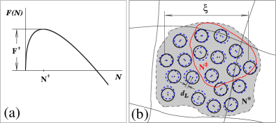
Figure 1: (a): Typical nucleation profile of one aperiodic lattice, within another, in deeply supercooled liquids. $N\equiv(4\pi/3)(r/a)^{3}$, $N^{\ddagger}$ is the typical transition state size: $(dF/dN)_{N^{\ddagger}}=0$. $\xi$ is the volumetrically defined cooperative length: $N^{*}\equiv(\xi/a)^{3}$, where $F(N^{*})=0$. (b): Cartoon of a structural rearrangement. The shown magnitude of $\xi$ corresponds to a temperature near $T_{g}$ on 1 hour scale. The two sets of circles - solid and dashed ones - denote two alternative structural states. $d_{L}\simeq a/10$, or the “Lindemann length”, is the typical bead displacement during a transition.

Once locally metastable, the liquid may reconfigure but in an activated fashion, i.e. by nucleating a new aperiodic structure within the present one. Such activated events occur, on average, once per typical $\alpha$-relaxation time $\tau$, per region of size $\xi$. The nucleus grows in a sequence of individual, nearly-barrierless bead moves of length $d_{L}\simeq a/10$ Singh et al. (1985); Lubchenko (2006) and time $\tau_{\mbox{\scriptsize micro}}\simeq 1$ ps Lubchenko (2006). The overall sequence of elemental moves typically corresponds to the following activation profile, see Fig.1(a):

$$F(N)=\gamma\sqrt{N}-Ts_{c}N,$$ (1)

where $N$ is the size of a reconfigured region. The “surface term” $\gamma\sqrt{N}$ is the mismatch penalty for creating one aperiodic structure within another. $s_{c}$ is the excess, “configurational” entropy of the liquid per bead, hence the entropic, bulk term $(-Ts_{c}N)$, which drives the transition and reflects the multiplicity of possible aperiodic arrangements in a region of size $N$. The maximum of the profile:

$$F^{\ddagger}=\mbox{max}\{F(N)\}=\frac{\gamma^{2}}{4s_{c}T}$$ (2)

is achieved at $N^{\ddagger}=N^{*}/4$, where $F(N^{*})=0$, so that the typical relaxation time is

$$\tau=\tau_{\mbox{\scriptsize micro}}e^{F^{\ddagger}/k_{B}T}\equiv\tau_{\mbox{\scriptsize micro}}e^{DT_{K}/(T-T_{K})}.$$ (3)

This formula works well at $\tau>1$ nsec or so. The form on the r.h.s. is the Vogel-Fulcher law, derived in the RFOT.

The end result of a cooperative, activated event is a reconfigured region of size $\xi$, where each of the $N^{*}\equiv(\xi/a)^{3}$ beads has moved the Lindemann length $d_{L}$, or so, see Fig.1(b). Both $\xi$ and the nucleation critical size, $r^{\ddagger}=\xi/4^{1/3}$, increase with lowering the temperature, roughly as $r^{\ddagger}\propto\xi\propto 1/(T-T_{K})^{2/3}$ Kirkpatrick et al. (1989); Xia and Wolynes (2000); Lubchenko and Wolynes (2003b). Here, $T_{K}$ is the so called ideal glass transition temperature, where the excess liquid entropy $s_{c}$, extrapolated below $T_{g}$, would vanish Kauzmann (1948). At $T_{g}$, $\xi$ is still quite modest, only about six beads across Xia and Wolynes (2000); Lubchenko and Wolynes (2001). Activated transport becomes dominant below the temperature $T_{\mbox{\scriptsize cr}}$, such that $r^{\ddagger}(T_{\mbox{\scriptsize cr}})=a$, which corresponds, apparently universally, to $\tau/\tau_{\mbox{\scriptsize micro}}\simeq 10^{3}$, or viscosities on the order of 10 Ps Lubchenko and Wolynes (2003b). At times shorter than $10^{3}\tau_{\mbox{\scriptsize micro}}$, one may then speak of a local aperiodic lattice on length scales of the cooperativity size $\xi$, since the slow structural reconfigurations have now time-scale separated from the vibrations Lubchenko and Wolynes (2003b). Because of the local nature of structural relaxations, one speaks of dynamic heterogeneity, or a “mosaic” of cooperative rearrangments Xia and Wolynes (2000). The heterogeneity is two-fold: On the one hand, a local rearrangment implies that the surrounding structure is static during the transition, up to vibrations. On the other hand, because of the spatial and temporal variation in the local density of states (and hence variations in $s_{c}$), local reconfigurations are generally subject to somewhat different barriers in different regions Xia and Wolynes (2000) (see Eq.(2) and also Section IV).

Computation of the viscosity in such a dynamically heterogeneous environment may be done in two steps: First compute the viscosity in a medium with a homogeneous relaxation time, call it $\tau^{\prime}$, and then average out with respect to the true distribution of the relaxation times. This procedure is valid in view of the equivalence of time and ensemble average. When the relaxation rate is strictly spatially homogeneous, one may formally define a diffusion constant for an individual bead: $D^{\prime}=d_{L}^{2}/6\tau^{\prime}$, since a bead moves the Lindemann length, once per time $\tau^{\prime}$, on average. Note that since a bead’s movements, as embodied in $d_{L}$ and $\tau^{\prime}$, are dictated by its cage, this is an example of “slaved” motion, to borrow Frauenfelder’s adjective for conformational changes of a protein encased in a stiff solvent Fenimore et al. (2002); Lubchenko et al. (2005). One may associate, by detailed balance, a low-frequency drag coefficient to that diffusion constant: $\zeta^{\prime}=k_{B}T/D^{\prime}$. Such dissipative response implies irreversible momentum exchange between a chosen particle and its homogeneous (!) surrounding, hence a Stokes’ viscosity $\eta^{\prime}=\zeta^{\prime}/(6\pi a/2)$, where $a/2$ is used for the radius of the region carved out in the liquid by a single bead. Averaging with respect to $\tau^{\prime}$ yields for the steady state viscosity of the actual heterogeneous liquid:

$$\eta=\frac{2k_{B}T}{\pi ad_{L}^{2}}\left\langle\tau\right\rangle,$$ (4)

where we have removed the prime at $\tau$, implying averaging with respect to the actual barrier distribution. The equation above can be rewritten as

$$\eta=(a/d_{L})^{2}\frac{2k_{B}T}{\pi a^{3}}\left\langle\tau\right\rangle\simeq 60\>\frac{k_{B}T_{g}}{a^{3}}\left\langle\tau\right\rangle,$$ (5)

since the Lindemann ratio, $d_{L}/a\simeq 0.1$ has been argued to change at most by 10% between $T_{m}$ and $T_{g}$ Lubchenko (2006).

Another instructive way to present Eq.(4) is to note that the Lindemann length is nearly equal to the typical amplitude of high-frequency vibrations: $d_{L}\simeq d_{\mbox{\scriptsize vibr}}$, within 5% or so, see Fig.3 of Ref.Lubchenko (2006). The vibrational amplitude is fixed by the equipartition theorem, since per bead: $K_{\infty}a^{3}(d_{\mbox{\scriptsize vibr}}/a)^{2}=k_{B}T$, where $K_{\infty}$ is the high-frequency elastic constant of the aperiodic lattice. One gets, as a result, a Maxwell-type expression:

$$\eta\sim K_{\infty}\left\langle\tau\right\rangle.$$ (6)

The last equation provides an easy way to see that the estimates in Eqs.(4)-(6) agree well with the experiment: Judging from the sound speed in glasses Freeman and Anderson (1986); Berret and Meissner (1988), the typical high frequency elastic modulus is about $10^{9}-10^{10}$ Pa, i.e. comparable but somewhat less than those of crystals. The range of relaxation times $10^{-12}-10^{4}$ sec, implies $10^{-3}-10^{13}$ Pa$\cdot$sec for the viscosity, as is indeed observed. Alternatively, one may obtain these figures by substituting a typical $a\sim 3$Å (see Lubchenko and Wolynes (2003b); Stevenson and Wolynes (2005) for specific estimates of bead sizes/densities).

Finally, the exploited equivalence between the time and ensemble averages implies that crystallization has not begun during the experiment, of course. The latter possibility adds uncertainty into viscosity measurements, as the presence of crystallites would greatly broaden the dynamic range of local relaxations owing to relatively slow crystal nucleation events and the slow hydrodynamics near the crystallites. Similarly, long chain motions in polymeric melts would also introduce additional long time scales into the problem. Our derivation does not apply to those situations. We note that optical transparency, which is often used as an indicator of no-crystallinity, does not ensure that crystallites - hundreds of nanometers across or smaller - are absent. Therefore a rigorous experimental study should, in the least, check whether performing viscoelastic measurements has enhanced the crystallization of the sample. Ideally, X-ray diffraction should be monitored in the course of viscosity measurements.

III Ionic Conductivity

In any supercooled melt, whether regarded ionic or not, the beads carry an additional charge, relative to the corresponding crystal, because of the lack of crystalline symmetry. As a result, each structural reconfiguration is characterized by a transition-induced electric dipole, see Fig.2.

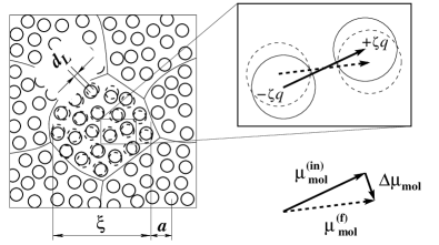
Figure 2: Shown on the left is a fragment of the mosaic of cooperatively reconfiguring regions in the supercooled liquid. Expanded portion shows how rotation of a bond leads to generating an elemental dipole change during a transition, where the partial charges on the two beads are $\pm\zeta q$.

The latter was estimated to be about a Debye or so, for most molecular substances Lubchenko et al. (2006). This value comes about as we may break up the whole domain into $N^{*}/2$ pairs, where is pair has an elemental dipole $\bm{\mu}_{i}$, $i=1\ldots N^{*}/2$: $\left\langle|\bm{\mu}_{i}|\right\rangle=\zeta eq$. Here $q$ is the elementary charge: $q=10^{0}e$, and $\zeta<1$ characterizes the excess charge. This quantity $\zeta$ is usually small reflecting small deviations from the crystalline symmetry, in the case of molecular crystals, or reflecting the weak interaction in Van der Waals systems. Alternatively, the overall density of charged/polar beads may be low. Ionic melts, by the very meaning of the term, are distinct from molecular/Van der Waals systems in that nearly all beads are strongly charged, implying $\zeta\sim 1$. To be more specific, the conclusions of this article will be exemplified with an often studied mixture of 40% Ca(NO₃)₂-60%KNO₃ (“CKN”), $T_{g}\simeq 330$K.

During a transition, each dipole turns by an angle $(d_{L}/a)$. The total transition dipole:

$$\bm{\mu}_{T}=\sum_{j}^{N^{*}/2}\left[\bm{\mu}_{j}^{(f)}-\bm{\mu}_{j}^{(in)}\right]$$ (7)

scales as $\sqrt{N^{*}}$ because of the random orientation of the elemental dipoles Lubchenko et al. (2006):

$$\mu_{T}\simeq\zeta(qa)[(\xi/a)^{3}/2]^{1/2}(d_{L}/a).$$ (8)

When the dipole density is uniform, every transition results in a local arrangement equally representative of the liquid structure. In other words, structural transitions do not modify the overall pattern of the immediate coordination shell. Transitions lead to a local ionic currents: $\bm{i}^{\prime}=\bm{\mu}_{T}^{\prime}/\tau^{\prime}$, per region of volume $\xi^{3}$. In the presence of an electric field, the net current density:

$$\bm{j}=\left\langle\bm{j}^{\prime}\right\rangle=\frac{1}{\xi^{3}}\left\langle\frac{\bm{\mu}_{T}}{\tau}\right\rangle,$$ (9)

is non-zero because the dipole moment at the transition state is correlated with the overall transition dipole moment. The latter can be shown using Wolynes’ library construction of liquid states Lubchenko and Wolynes (2004a). Repeating that argument, but in the presence of electric field $\bm{E}$, yields for the typical free energy profile for structural reconfiguration in steady state:

$$F(N)=\gamma\sqrt{N}-\bm{\mu}_{T}(N)\bm{E}_{c}-Ts_{c}N,$$ (10)

where $N$ is the size of the rearranged region and

$$\bm{\mu}_{T}(N)=\sum_{j}^{N/2}\left[\mu_{j}^{(f)}-\mu_{j}^{(in)}\right]$$ (11)

is the overall dipole change in that region. The subscript “$c$” in $\bm{E}_{c}$ signifies that the latter is a cavity field. The field dependent term $|\bm{\mu}_{T}(N)\bm{E}_{c}|\ll k_{B}T$ is overwhelmingly smaller than the other terms in Eq.(10). As a result, the transition state dipole moment is not field-induced, but, again, is “slaved” to the lattice. More formally, one may use the argument from Ref.Lubchenko and Wolynes (2001) showing that the density of structural states at the reconfiguration bottle-neck is of the order $1/T_{g}$, implying the field will not affect the specific sequence of elemental moves, but will affect the dynamics merely by shifting the energies along structurally dictated sequences of moves. Thus in the lowest order in $\bm{E}_{c}$, $\tau^{-1}(\bm{E}_{c})=\tau^{-1}(\bm{E}_{c}=0)(1+\bm{\mu}_{T}^{\ddagger}\bm{E}_{c}/k_{B}T)$, yielding

$$\bm{j}=\left\langle\frac{\bm{\mu}_{T}(\bm{\mu}_{T}^{\ddagger}\bm{E}_{c})}{\tau}\right\rangle\frac{1}{k_{B}T},$$ (12)

where $\bm{\mu}_{T}^{\ddagger}\equiv\bm{\mu}_{T}(N^{\ddagger})$ is the transition dipole moment at the zero-field transition state. The cavity field, see e.g. Titulaer and Deutch (1974), is related to the external field $E^{(\infty)}$ by

$$E_{c}(\omega)=E^{(\infty)}(\omega)\frac{3\epsilon_{b}(\omega)}{2\epsilon_{b}(\omega)+1},$$ (13)

where $\epsilon_{b}(\omega)$ is the dielectric constant of the surrounding bulk. Since a steady current is implied in the derivation, (the imaginary part of) $\epsilon_{b}(\omega)$ diverges at zero frequency, implying $E_{c}=E^{(\infty)}(3/2)$. One thus obtains for the ionic conductivity tensor:

$$\sigma_{ij}=\left\langle\frac{(\bm{\mu}_{T})_{i}(\bm{\mu}_{T}^{\ddagger})_{j}}{\tau}\right\rangle\frac{3}{2k_{B}T\xi^{3}}.$$ (14)

Bearing in mind that $N^{\ddagger}=N^{*}/4=(\xi/a)^{3}/4$, and that the liquid is isotropic, on average: $\left\langle(\Delta\bm{\mu})_{i}(\Delta\bm{\mu})_{j}\right\rangle=\delta_{ij}(\Delta\mu)^{2}/3$, one finally has:

$$\sigma_{ij}=\delta_{ij}\,\frac{\Delta\mu_{\mbox{\scriptsize mol}}^{2}}{8\,a^{3}k_{B}T}\left\langle\frac{1}{\tau}\right\rangle,$$ (15)

where

$$\Delta\mu_{\mbox{\scriptsize mol}}^{2}\equiv\left\langle\left[\mu_{j}^{(f)}-\mu_{j}^{(in)}\right]^{2}\right\rangle$$ (16)

is the average elemental dipole change squared. Finally note that in covalently networked materials, where dipole assignment may be ambiguous, one may still estimate local dipole changes using the known piezoelectric properties of the corresponding crystal, see Lubchenko et al. (2006) for details.

The derivation above does not apply to systems where the dipole density is significatly non-uniform. For instance, glycerol has one polar, OH group per non-polar, aliphatic group, implying the liquid is non-homogeneous, dipole moment wise, on the $\alpha$-relaxation time scale. In such systems, the premise that structural rearrangements result in equally representative configurations of the liquid does not hold. In the glycerol example, ionic conduction would imply breaking OH or CH bonds. In CKN, on the other hand, the overall bond pattern, around any atom, does not change significantly during a transition, even though individual bonds distort by the Lindemann length, as mentioned. Eq.(15) thus places the absolute upper limit on the intrinsic ionic conductivity of a melt. By “intrinsic” we mean that the computed currents are always present in the fluid and result from the intrinsic activated transport: Local bond pattern does not change significantly in the course of an individual activated event, but only in the course of many consecutive events, since during an individual event, the molecular displacements barely exceed typical vibrational displacements. Conversely, if a system displays a higher conductivity than prescribed by Eq.(15), one may conclude that the ion motion does not require structural reconfiguration. Here, the bond pattern actually changes, however these are not scaffold bonds of the aperiodic lattice comprising the fluid (or glass). (More on this below.)

To simplify comparison of Eq.(15) with experiment, let us express the combination of the bead charge $\zeta q$ and size $a$, in Eq.(15), through the finite frequency dielectric response, a measurable quantity in principle (see below). The latter is the response of a rearranging region in the absence of bulk current, i.e. with a fixed environment, up to vibrations. It is convenient to choose such regions at volume $\xi^{3}$, so that each region has two structural states available, within thermal reach from each other, separated by a barrier sampled from the actual barrier distribution in the liquid. If the two states, “1” and “2” are characterized by dipole moments $\bm{\mu}_{1}$ and $\bm{\mu}_{2}$ respectively, the expectation value of the dipole moment of the region is $\mu=(\bm{\mu}_{1}+\bm{\mu}_{2})/2+\Delta\bm{\mu}(p_{2}-p_{1})/2$, where $\Delta\bm{\mu}\equiv(\bm{\mu}_{2}-\bm{\mu}_{1})$; $p_{1}$ and $p_{2}=(1-p_{1})$ are the probabities to occupy state 1 and 2 respectively. The relative population $(p_{2}-p_{1})$ depends on the field via $\delta\ln(p_{2}/p_{1})=\Delta\bm{\mu}\bm{E}_{c}/k_{B}T$. At realistic field strengths, i.e. $|\Delta\bm{\mu}\bm{E}_{c}/k_{B}T|\ll 1$, one has for the field-induced shift of the relative population: $\delta(p_{2}-p_{1})\simeq 2p_{1}p_{2}(\Delta\bm{\mu}\bm{E}_{c})$. Similarly to the preceding argument, $\left\langle(\Delta\bm{\mu})_{i}(\Delta\bm{\mu})_{j}\right\rangle=(N^{*}/2)\delta_{ij}(\Delta\mu_{\mbox{\scriptsize mol}})^{2}/3$. Further, since we have frozen the structural transitions in the surrounding region, in estimating the cavity field, one must use $\epsilon(\omega)$ with the $\alpha$-relaxation contribution subtracted. This does not introduce much ambiguity because in most ionic substances, the dielectric constant even at very high frequences is significantly larger than unity. In CKN, for instance, $\epsilon^{\prime}(\infty)\simeq 7$ Howell et al. (1974), allowing us to write as before: $E_{c}\simeq E^{(\infty)}(3/2)$. One thus obtains, in a standard fashion, for the frequency dependent dielectric constant in the absence of macroscopic current:

$$\epsilon_{\mbox{\scriptsize ins}}(\omega)-\epsilon_{\infty}=4\pi\left\langle p_{1}p_{2}\right\rangle\frac{\Delta\mu_{\mbox{\scriptsize mol}}^{2}}{4\,a^{3}k_{B}T}\left\langle\frac{1}{1-i\omega\tau}\right\rangle,$$ (17)

where the label “ins” signifies the absence of dc conductivity.

In the presence of steady current, the full response per domain is the sum of the steady current from Eq.(15) and the ac current from Eq.(17). The addition of the dc contribution, $i\sigma/\omega$, to the full dielectric response will increase the absolute value of $\epsilon_{b}(\omega)$. This means that Eq.(17) should work even better. One thus gets for the full dielectric response of a conducting substance:

$$\epsilon(\omega)-\epsilon_{\infty}=4\pi\left\langle p_{1}p_{2}\right\rangle\frac{\Delta\mu_{\mbox{\scriptsize mol}}^{2}}{4\,a^{3}k_{B}T}\left\langle\frac{1}{1-i\omega\tau}\right\rangle+i\frac{\sigma}{\omega},$$ (18)

where $\sigma$ is the dc conductivity from Eq.(15).

One needs to know the distribution of the transition energies $E$ to estimate the quantity $\left\langle p_{1}p_{2}\right\rangle\equiv\left\langle 1/4\cosh^{2}(E/2k_{B}T)\right\rangle$. Since $\xi$ is the smallest possible size of a rearranging unit, these rearrangments correspond to the elementary excitations in the system. We thus conclude, based on equipartition, that the typical value of $E$ is roughly $k_{B}T$, implying that $\left\langle p_{1}p_{2}\right\rangle$ is close to its maximum value of one quarter but is likely smaller by another factor of two or so. Assuming then, for the sake of argument that $\left\langle p_{1}p_{2}\right\rangle=1/8$, one gets $\frac{\Delta\mu_{\mbox{\scriptsize mol}}^{2}}{a^{3}k_{B}T}\simeq 2(\epsilon^{\prime}_{0}-\epsilon_{\infty})$, within an order of magnitude. By Eq.(15), this implies a Maxwell-like relation between the dc conductivity and the real part of the dielectric response:

$$\sigma\sim(\epsilon^{\prime}_{0}-\epsilon_{\infty})\left\langle\frac{1}{\tau}\right\rangle,$$ (19)

with an important distinction, though, that here one averages the inverse relaxation time. The $(\epsilon^{\prime}_{0}-\epsilon_{\infty})$ difference in CKN, to be concrete, is about $(20-7)=13$ Pimenov et al. (1995); Howell et al. (1974). This implies, by Eq.(17) and CKN’s $T_{g}\simeq 330$K Pimenov et al. (1995), that $\zeta q\simeq 3e$, at $a=3$Å, a reasonable value for the bead charge. Note that $a=3$Å is consistent with CKN’s $\Delta c_{p}\simeq.12$ cal/g K Angell and Torell (1983) and the mentioned $D=32/\Delta c_{p}$ Xia and Wolynes (2000).

Now, substituting CKN’s $(\epsilon^{\prime}_{0}-\epsilon_{\infty})$ into Eq.(15) yields for the conductivity $\sigma\simeq 3\cdot 10^{-10}\left\langle\tau^{-1}\right\rangle$ (Ohm m)^-1sec. Naively replacing $\left\langle\tau^{-1}\right\rangle$ with $1/\left\langle\tau\right\rangle$ would imply, at the glass transition, where $\left\langle\tau\right\rangle\sim 10^{2}-10^{3}$ sec, a conductivity of the order $10^{-13}-10^{-14}$ (Ohm cm)^-1, which is three to four orders of magnitude below the observed value Pimenov et al. (1995); Howell et al. (1974). Note that the value $\left\langle\tau^{-1}\right\rangle\left\langle\tau\right\rangle=10^{3}-10^{4}$ is just the magnitude of decoupling observed in CKN near $T_{g}$ Howell et al. (1974); Angell (1990), and is in fact expected for a fragile substance such as CKN is, as we will argue in the following.

IV Barrier distribution and the Decoupling

Relaxation barriers in supercooled liquids are distributed because the local density of states is non-uniform, leading to variations in the local value of the configurational entropy and hence the RFOT-derived barrier from Eq.(2). In the simplest argument, the gaussian fluctuations of the entropy translate into gaussian fluctuations in the barrier, where the relative deviations of the two quantities, from the most probable value, are given by Xia and Wolynes (2001a):

$$\delta\widetilde{F}\equiv\frac{\delta F}{F_{\mbox{\scriptsize mp}}}=\frac{\delta s_{c}}{s_{c}}=\frac{1}{2\sqrt{D}},$$ (20)

where $D$ is the liquid’s fragility from Eq.(3). The quantity $1/2\sqrt{D}$ varies between 0.05 and 0.25 or so, for known glassformers, the low and high limits corresponding to strong and fragile substances respectively.

Xia and Wolynes (XW) further argued that the real barrier distribution should be cut-off at the most probable value because a liquid region with relatively low density of states is likely neighbors with a relatively fast region Xia and Wolynes (2001a). In addition we may recall that in the library construction, the most likely liquid state is the one where the liquid is guaranteed to have an escape trajectory Lubchenko and Wolynes (2004a). This means that the most probable barrier is also the maximum barrier. One may conclude then that the naive Gaussian distribution is adequate at small barriers, but significantly overestimates the probability of barriers larger than the typical barrier. Put another way, the trajectories corresponding to higher than most probable barrier in the naive Gaussian, all contribute to the $F\leq F_{\mbox{\scriptsize mp}}$ range. XW have implemented this notion by replacing the r.h.s. of the simplest Gaussian distribution by a delta-function centered at $F_{\mbox{\scriptsize mp}}$ Xia and Wolynes (2001a):

$$p_{1}(\widetilde{F})=\frac{e^{-(1/\widetilde{F}-1)^{2}/2\delta\widetilde{F}^{2}}}{\sqrt{2\pi(\delta\widetilde{F})^{2}}\widetilde{F}^{2}}+\frac{1}{2}\delta(\widetilde{F}-1),$$ (21)

where $\widetilde{F}\equiv F/F_{\mbox{\scriptsize mp}}<1^{+}$, and we took advantage of the temperature-independence of the relative width in Eq.(20). This approximate form does not use adjustable parameters and quantitatively accounts for the correlation between the fragility and the stretching exponent $\beta$ Xia and Wolynes (2001a), and the deviations from the Stokes-Einstein relation. The distribution in Eq.(21) is shown in Fig.3. The only difference of Eq.(21) with the XW’s form is that they used a purely gaussian form for $\widetilde{F}<1$, whereas we follow their own suggestion and employ the more accurate $F\propto 1/s_{c}$ (where $s_{c}$ is gaussianly distsributed of course). The accurate evaluation of the left wing of the distribution is imperative in estimating the average rate $\tau_{\mbox{\scriptsize micro}}^{-1}e^{-F/k_{B}T}$, because the latter is a rapidly varying function of $F$. ($k_{B}T$ is significantly less that $\delta F$ at low temperatures.) Note that because of the rapid decay of the exponential at small $\widetilde{F}$ in Eq.(21), accounting for the lowest order, quadratic fluctuations of entropy suffices. The quantity $\left\langle\tau\right\rangle\left\langle\tau^{-1}\right\rangle$, that characterizes the apparent decoupling, computed with the XW’s distribution, is shown with the dashed line in Fig.4, at $T_{g}$, as a function of the relative distribution width $\delta\widetilde{F}$.

How robust is the prediction based on the simple functional form for the barrier distribution from Eq.(21)? In spite of its quantitative successes, one may argue that the true barrier distribution should be a smoother function, near $\widetilde{F}=1$. One way to see this is to computing $\epsilon^{\prime\prime}(\omega)$ from Eq.(17) via the distribution in Eq.(21): The obtained curves are a sum of two peaks, one of which is broader, one the other is narrower than the experimental $\epsilon^{\prime\prime}(\omega)$. The two peaks correspond to the half-Gaussian and the delta-function in Eq.(21) respectively. Let us see that knowing the precise form of the barrier distribution however is not essential in quantitative estimates of the decoupling so long as we account correctly for the overall width of the distribution and its decay at the low barrier side.

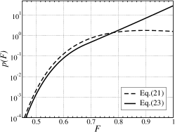
Figure 3: The barrier distributions from Eqs.(21) and (23). The $\delta$-function portion of the distribution from Eq.(21) is not shown. $\delta\widetilde{F}=0.25$.

It is straightforward to show that there exists a distribution that (a) satisfies these requirements without introducing adjustable constants, (b) reproduces the experimental $\epsilon(\omega)$ and does as well as the XW form for the $\beta$ vs. $D$ correlation. As we have already discussed, the low barrier wing of the distribution in Eq.(21) is adequate. On the other hand, the high barrer wing should include the contributions from both sides of the original Gaussian peak, which are both of width $\delta F/2$. “Stacking” these two on top of each other, to the left of $F_{\mbox{\scriptsize mp}}$, results in a distribution of width $\delta F/4$ (see aslo Appendix). Further, based on the known $\epsilon(\omega)$ data, the barrier distribution should be well approximated by an exponential, suggesting we use $p(F)\propto e^{F/(\delta F/4)}$ near $F_{\mbox{\scriptsize mp}}$. Indeed, this implies $p(\tau)\propto\tau^{(4k_{B}T/\delta F)-1}$. At frequencies not too close to the maximum of $\epsilon^{\prime\prime}(\omega)$ and the rapid drop-off at small $\widetilde{F}$, one has an approximate power law:

$$\epsilon^{\prime\prime}(\omega)\simeq\int_{0}^{\infty}d\tau\,\tau^{(4k_{B}T/\delta F)-1}\frac{\omega\tau}{1+(\omega\tau)^{2}}\propto\omega^{-4k_{B}T/\delta F}.$$ (22)

We thus arrive at the following form:

$$p(\widetilde{F})=\left\{\begin{array}[]{ll}\frac{c_{1}}{\widetilde{F}^{2}}e^{-(1/\widetilde{F}-1)^{2}/2\delta\widetilde{F}^{2}},&\widetilde{F}\leq\widetilde{F}_{e}\\ \frac{c_{2}}{\widetilde{F}^{2}}e^{\widetilde{F}/(\delta\widetilde{F}/4)},&\widetilde{F}_{e}<\widetilde{F}\leq 1,\end{array}\right.$$ (23)

where $F_{e}$ and the normalization constants $c_{1}$ and $c_{2}$ are chosen so that the distribution is normalized, continuous, and its first derivative is continuous too. The distribution from Eq.(23) is plotted in Fig.3. The decoupling strength $\left\langle\tau\right\rangle\left\langle\tau^{-1}\right\rangle$, computed for the composite distribution from Eq.(23), is shown in Fig.4, as a function of the relative distribution width $\delta\widetilde{F}$, at $T_{g}$. We therefore observe that in fragile liquids, the apparent time-scale separation may reach as much as four orders of magnitude near the glass transition - even though only one process is present! - because the inrinsic ionic conductivity is dominated by the fastest relaxing regions.

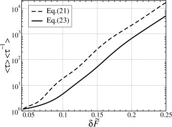
Figure 4: The decoupling between the viscosity and the intrinsic ionic conductivity, as a function of the relative barrier width $\delta\widetilde{F}$ from Eq.(20), at $T_{g}$. The dashed and solid line pertain to the specific barrier distributions from Eq.(21) and (23) respectively.

Conversely, when the apparent decoupling exceeds the intrinsic value prescribed by Fig.4, we may conclude that ionic conduction does not in fact require structural relaxation. This notion is of significance for the mechanisms of electrical conductance in glasses and will be discussed in detail in the Conclusions.

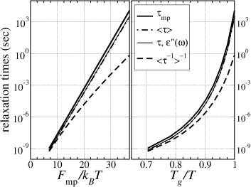
Figure 5: Different relaxation times derived from the barrier distribution in Eq.(23), as functions of the most probable barrier (left) and the corresponding temperature (right). $\delta\widetilde{F}=0.25$, corresponding to fragility $D=4$.

One may also illustrate the effects of apparent decoupling for a specific value of fragility, by plotting several varieties of relaxation times, as functions of the most probable barrier, or the corresponding temperature, see Fig.5. (Given the time scale at the glass transition, say $DT_{K}/(T_{g}-T_{K})=\ln(10^{16})\simeq 37$ (see Eq.(3)), there is a one-to-one correspondence between the fragility $D$ and the $T_{g}/T_{K}$ ratio.) We observe that the average relaxation time and the one derived from the inverse of the maximum position of $\epsilon^{\prime\prime}(\omega)$ are close, and are near the most probable value of the relaxation time. (The $\epsilon^{\prime\prime}(\omega)$ was computed using Eqs.(18) and (23), see below.) The apparent conductivity relaxation time is strongly decoupled, consistent with data of Howell at el. Howell et al. (1974) for CKN. Note that the value of fragility used in Fig.5, $D=2$, is probably smaller than in CKN. In addition, we have ignored here, for clarity, the effects of barrier softening Lubchenko and Wolynes (2003b), that would require introducing a system-specific adjustable constant $T_{A}$. The latter effects would change the slopes of the curves somewhat, without affecting their vertical separations.

To test the predictions from Figs.4 and 5, one needs to know the width of the barrier distribution for $\alpha$-relaxation. As already mentioned, the gross features of this distribution have been predicted by the RFOT theory, and have lead to quantitative predictions of the correlation between the stretching exponent $\beta$ and the fragility $D$, and the deviations from the Stokes-Einstein relation. The corresponding trends are as follows: more fragile liquids are predicted to have broader barrier distribution leading to a smaller value of $\beta$, and vice versa for stronger substances Xia and Wolynes (2001a). A correlation with the fragility comes about by virtue of Eq.(20). Several à priori ways to determine $\beta$ and $D$ have been employed, by experimenters, that sometimes produce conflicting results. For example, the fragility extracted from $\tau_{\sigma}$ will be consistently lower than that extracted from the mechanical relaxation time $\tau_{s}$, because $\tau_{\sigma}<\tau_{s}$. The exponent $\beta$ from the stretched exponential is extracted from fits of various relaxation processes to a stretched exponential profile $e^{-(t/\tau)^{\beta}}$. Alternatively, one may choose to fit the Fourier transform of the stretch exponential, or the Cole-Davidson form, to the imaginary part of $\epsilon(\omega)$ in insulators Lindsey and Patterson (1980). These usually produce comparable results for the corresponding exponent $\beta$, with a notable exception of ionic conductors, which happen to be the main focus of this paper. In ionically conducting systems, the dc component of the full dielectric response from Eq.(18) largely “swamps” the ac part so that reliable determinations of the latter are complicated. The reader is reminded that dielectric measurements on ion melts are difficult because electrodes generally block ionic current. The effects of build-up charge are often treated phenomenologically, by means of equivalent circuits Macdonald (1987); Pimenov et al. (1995). Given these complications, many have chosen to plot the reciprocal of $\epsilon(\omega)$, i.e. the dielectric modulus Howell et al. (1974); Macdonald (1987):

$$M(\omega)\equiv 1/\epsilon(\omega).$$ (24)

$M(\omega)$ is well behaved and even shows a peak in the imaginary component, similarly to $\epsilon(\omega)$ of a near insulator. In the absence of an à priori microscopic picture and by analogy with $\epsilon(\omega)$, one might interpret this peak as as the response of the electric field $\bm{E}$ to the dielectric displacement $\bm{D}$. This in fact would be appropriate in a layered dielectric Howell et al. (1974). See also the discussions in Refs.Elliott (1994); Roling (1998); Cole and Tombari (1991); Sidebotom et al. (1995); Moynihan (1994); Dyre (1991); Doi (1988). Yet the resulting values of the most probable relaxation time and the stretching exponent deviate from those obtained with other methods Angell (1990); Sidebotom et al. (1995); Pimenov et al. (1995). In fact, the modulus-derived $\beta_{M}$ increases, while the width of the $M^{\prime\prime}(\omega)$ peak decreases with lowering the temperature, in conflict with the general trends for poor conductors, and the conclusions of the RFOT theory.

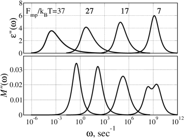
Figure 6: The top panel shows the imaginary part of the non-conductive part of the dielectric response, $\epsilon(\omega)$, Eq.(17), for four values of the most probable $\alpha$-relaxation barrier: $F_{\mbox{\scriptsize mp}}/k_{B}T=\ln(\tau/\tau_{\mbox{\scriptsize micro}})$, as indicated on the graph. ($\delta\widetilde{F}=0.25$, $\tau_{\mbox{\scriptsize micro}}=1$ ps.) These barrier values were chosen because for $\tau/\tau_{\mbox{\scriptsize micro}}>e^{7}\simeq 10^{3}$, the RFOT approach is quantitatively accurate, while $\tau/\tau_{\mbox{\scriptsize micro}}\simeq e^{37}\simeq 10^{16}$ is at the upper limit of the dynamical range routinely accessible in the lab. The bottom panel show the corresponding modulus, from Eq.(24), that includs the dc-part, due to the intrinsic ionic current. The same four values of the barrier are used. We have used the CKN’s values for $\epsilon_{0}$ and $\epsilon_{\infty}$, and assumed that $\frac{\Delta\mu_{\mbox{\scriptsize mol}}^{2}}{a^{3}k_{B}T}\simeq 2(\epsilon^{\prime}_{0}-\epsilon_{\infty})$, see the discussion preceeding Eq.(19).

The RFOT theory and the present results allow one to address these difficulties, to which we devote the rest of this Section. One first notes that structural reconfigurations are compact, and so the layered-dielectric view of supercoold melts is not microscopically justified. We next plot, in the top panel of Fig.6, the non-conductive $\epsilon_{\mbox{\scriptsize ins}}^{\prime\prime}(\omega)$, from Eq.(17) averaged with respect to the barrier distribution from Eq.(23). We have used CKN’s values for $\epsilon_{0}$ and $\epsilon_{\infty}$, as before. For the sake of argument, we use $\delta\widetilde{F}=0.25$, corresponding to $\beta\simeq 0.4$ at $T_{g}$. In Fig.6, bottom, we show the imaginary part $M^{\prime\prime}(\omega)$, of the full modulus. Clearly the two functions exhibit qualitatively different behaviors. Note that the effect of the dc component on the apparent relaxation profile has been discussed previously Johari and Pathmanathan (1988); Roling (1998), including the possibility of a double peak Johari and Pathmanathan (1988). The latter has been observed by Funke at el. Funke et al. (1988), but has not been reproduced by Pimenov at el. Pimenov et al. (1995). Nevertheless, the dielectric modulus obtained here is qualitatively consistent with CKN’s data from Ref.Pimenov et al. (1995). Finally note that for smaller dc-conductivities, the modulus data would become more similar to $\epsilon^{\prime\prime}(\omega)$.

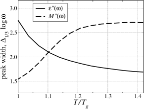
Figure 7: The widths of the peaks in the imaginary parts of the dielectric constant $\epsilon(\omega)$ and modulus $M(\omega)$, as functions of temperature (c.f. Fig.6). $\delta\widetilde{F}=0.25$.

We conclude from the above analysis that if one were to use the modulus data to extract the characteristics of the barrier distribution, one must measure first the dc-current, add it to the $\epsilon_{\mbox{\scriptsize ins}}(\omega)$ from a microscopic theory, and then compare the result to the measured $M(\omega)$ data. But again, because of the large contribution of the dc component, the corresponding fits would not discriminate well between different forms of $\epsilon_{\mbox{\scriptsize ins}}(\omega)$. On the other hand, treating the electric field as a response to the displacement may lead to erroneous conclusions on the temperature dependence of the barrier width. In fact, the barrier widths derived from $\epsilon_{\mbox{\scriptsize ins}}^{\prime\prime}(\omega)$ or $M^{\prime\prime}(\omega)$ show the opposite trends, as we have seen already in Fig.6. One may further quantify this observation: In the absence of a microscopic theory, one often characterizes the width of the $\epsilon_{\mbox{\scriptsize ins}}^{\prime\prime}(\omega)$ peak by a stretching exponent $\beta$, as derived e.g. from Davidson-Cole fits. The distribution from Eq.(23) indeed gives rise a power law behavior, consistent with Eq.(22), see Appendix. In contrast, the corresponding $M^{\prime\prime}(\omega)$ curves do not exhibit a similar power-law behavior. I have chosen to illustrate the opposite temperature trends in the widths of $\epsilon_{\mbox{\scriptsize ins}}^{\prime\prime}[\ln(\omega)]$ and $M^{\prime\prime}[\ln(\omega)]$ peaks, by measuring the latter widths at one-third-height and plotting them as functions of temperature, see Fig.7. Similar opposite trends, too, would be observed for the corresponding apparent barrier widths or effective $\beta$’s. Clearly, interpreting the dielectric modulus of an ionic conductor as a response function may lead to a significant underestimation of the actual barrier width at low temperatures, and qualitatively incorrect conclusions on the temperature dependence of the width.

V Conclusions

We have computed, from the first principles, the viscosity and the intrinsic ionic conductivity of supercooled liquids. The viscosity is determined by four microscopically defined quantities: the length scale of the local chemical order that sets in at temperature $T_{\mbox{\scriptsize cr}}$, where liquid dynamics become activated; the Lindemann length, characterizing molecular displacements at the mechanical stability edge; the temperature; and the average relaxation time $\tau$ of the activated reconfigurations that dominate the liquid dynamics below $T_{\mbox{\scriptsize cr}}$. The extraordinarily long $\tau$ range is what gives rise to the high viscosity of the liquid when it approaches the glass transition. When the local chemically stable units (or “beads”) are charged, the fluid will also exhibit an ionic conductivity, which we have called the “intrinsic” conductivity, to constrast it with electric conduction via delocalized electronic carriers or via mobile ions that are not bonded to the metastable aperiodic lattice forming the supercooled liquid. Computing the conductivity requires an additional microscopic characteristic, the electric charge on a “bead”. Fortunately, this additional parameter may be deduced from the ac dielectric response, which we have also estimated. Perhaps the main finding of this work is that in contrast with the viscosity, the ionic conductivity is dominated by the fastest relaxing regions in the liquid, as reflected in Eq.(15).

We have discussed ways to test the above predictions, the most important aspect of which is the large separation, or “decoupling”, between the apparent time scales, suggested previously by viscosity and ionic conductivity data on purely phenomenological grounds. We have shown that such apparent time-scale separation is indeed expected because of the very broad barrier distribution for $\alpha$-relaxation, derived earlier in the Random First Order Transition (RFOT) methodology. The decoupling thus stems essentially from the same cause as the violation of Stokes-Einstein relation in supercooled liquids Xia and Wolynes (2001b). Now, we have seen that the value of the decoupling is not very sensitive to the precise form of the barrier distribution so long as one acounts for the RFOT-derived gross characteristics of this. We have thus quantified the degree of “decoupling”: The intrinsic ionic conductivity was argued to decouple at most by four orders of magnitude from the low-frequency momentum transport. Conversely, any conductivity exceeding this limit must be due to other charge carriers that do not disturb the liquid structure beyond typical vibrational displacements. Indeed, suppose the apparent decoupling exceeds the value prescribed by the width of the barrier distribution. This means that there will be ions that travel a distance exceeding the Lindemann length in a time it takes the local environment to relax. Therefore, local relaxation is not a necessary condition for a non-zero current of these ions. Some interaction with relaxation may still be present, however at large enough decouplings, we may say that the ion (or any other carrier) interacts with the liquid as if the latter were a perfectly stable, albeit disordered lattice. In such cases, one may think of the ionic current in superionic conductors in terms of regular, not slaved diffusion. In regular diffusion, the total travel time is dominated by the slowest step, in contrast to Eq.(15).

The intrinsic difficulty in experimental assessment of the barrier distribution in moderately conductive melts is that the dc current dominates the overall dielectric response. This gives rise to ambiguities as to what the actual width of the barrier distribution is, since mechanical relaxation and dielectric modulus data disagree. We have shown that this is expected, and argued that the mechanical relaxation offers the preferred method of estimating the actual barrier distribution.

Acknowledgments: The author thanks Peter G. Wolynes for critical comments and useful suggestions. He gratefully acknowledges the GEAR, the New Faculty Grant, and the Small Grant Programs at the University of Houston.

Appendix

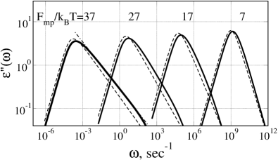
Figure 8: The four thick lines are the same as in Fig.6, but in the double-log scale. The thin lines are the Davidson-Cole forms, following from a simple approximation, see Appendix. The dash-dotted line illustrates how the stretching exponent $\beta$ was extracted from the curves.

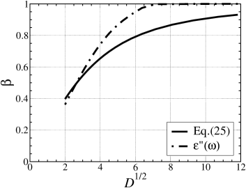
Figure 9: Two approximate relations of the stretching exponent $\beta$ to the fragility $D$ from the Vogel-Fulcher form, from Eq.(25) and as derived from the slopes of the high-frequency wing of the $\epsilon^{\prime\prime}(\omega)$ peaks, such as in Fig.8.

Let us see that the distribution in Eq.(23) is qualitatively consistent with experimental $\epsilon_{\mbox{\scriptsize ins}}(\omega)$ and the empirical correlation of $\beta$ and $D$. For this, we replot the top panel of Fig.6 in the double-log format, in Fig.8. We note the general adequacy of the barrier distribution from Eq.(23): Similarly to the experimental $\epsilon(\omega)$ in poor conductors, the resulting high-frequency wing is significantly broader than the low-frequency one. Note that the actual data would also often display an additional high-frequency wing, which is ascribed to the secondary, $\beta$-processes, also called Johari-Goldstein relaxation Johari and Goldstein (1970). (See Lunkenheimer and Loidl (2002) for a review). The present results suggest that $\beta$-relaxation does not contribute to the intrinsic ionic conductivity. At any rate, the derived $\epsilon(\omega)$ show several decades of nearly power-law decay, allowing one to extract the corresponding exponent: $\epsilon(\omega)\propto\omega^{-\beta}$. The effective $\beta$’s were deduced from the slopes of the curves at the points of maximum second derivative, as exemplified by the dash-dotted line in Fig.8. The dependence of the thus obtained exponent $\beta$ on the fragility $D$, at a fixed $F_{\mbox{\scriptsize mp}}/k_{B}T=37$, is shown by the dashed-dotted line in Fig.9. This $\beta$ is, again, qualitatively consistent with experiment. Greater accuracy should not be expected here, as we have not treated the higher-frequency range associated with $\beta$-relaxation, which would affect the experimentally determined stretching exponents.

In addition, we verify that the informal argument in the main text that the width of the barrier distribution should be about $\delta F/4$, at the half-height or so. Indeed, for a gaussian barrier distribution with width $\delta F/4=F/8\sqrt{D}$ implies the following approximate expression for the stretching exponent $\beta$ at $T_{g}$ (c.f. Eq.(9) of Ref.Xia and Wolynes (2001a)):

$$\beta=\left[1+\left(\frac{F/k_{B}T}{8\sqrt{D}}\right)^{2}\right]^{-1/2},$$ (25)

shown as the solid line in Fig.9. This expression is in very good agreement with experiment, see Fig.2 from Ref.Xia and Wolynes (2001a). (At $T_{g}$ on scale $\tau/\tau_{\mbox{\scriptsize micro}}=10^{16}$, $F/k_{B}T\simeq 37$.) Note also Eq.(25) is consistent with Eq.(20), assuming the Davidson-Cole Davidson and Cole (1950) and William-Watts Williams and Watts (1970) stretching exponents $\beta$ are close Lindsey and Patterson (1980). That the latter is the case indeed I demonstrate by graphing the Davidson-Cole (DC) form $(\epsilon_{{\mbox{\tiny DC}}}(\omega)-\epsilon_{\infty})=(\epsilon_{0}-\epsilon_{\infty})(1-i\omega\tau)^{-\beta}$ Davidson and Cole (1950) with $\tau=\tau_{\mbox{\scriptsize micro}}e^{F_{\mbox{\scriptsize mp}}/k_{B}T}$ and $\beta$ from Eq.(25). These are shown in Fig.8 as thin dashed lines.

References

- Kirkpatrick et al. (1989) T. R. Kirkpatrick, D. Thirumalai, and P. G. Wolynes, Phys. Rev. A 40, 1045 (1989).
- Xia and Wolynes (2000) X. Xia and P. G. Wolynes, Proc. Natl. Acad. Sci. 97, 2990 (2000).
- Xia and Wolynes (2001a) X. Xia and P. G. Wolynes, Phys. Rev. Lett. 86, 5526 (2001a).
- Xia and Wolynes (2001b) X. Xia and P. G. Wolynes, J. Phys. Chem. 105, 6570 (2001b).
- Lubchenko and Wolynes (2004a) V. Lubchenko and P. G. Wolynes, J. Chem. Phys. 121, 2852 (2004a).
- Lubchenko and Wolynes (2001) V. Lubchenko and P. G. Wolynes, Phys. Rev. Lett. 87, 195901 (2001).
- Lubchenko and Wolynes (2003a) V. Lubchenko and P. G. Wolynes, Proc. Natl. Acad. Sci. 100, 1515 (2003a).
- Lubchenko and Wolynes (2004b) V. Lubchenko and P. G. Wolynes (2004b), to appear in Adv. Chem. Phys.; cond-mat/0506708.
- Lubchenko and Wolynes (2006) V. Lubchenko and P. G. Wolynes, Annu. Rev. Phys. Chem. 58, 235 (2006), eprint cond-mat/0607349.
- Macedo et al. (1972) P. B. Macedo, C. T. Moynihan, and R. Bose, Phys. Chem. Glasses 13, 171 (1972).
- Howell et al. (1974) F. S. Howell, R. A. Bose, P. B. Macedo, and C. T. Moynihan, J. Phys. Chem. 78, 639 (1974).
- McLin and Angell (1988) M. McLin and C. A. Angell, J. Phys. Chem. 92, 2083 (1988).
- Angell (1990) C. A. Angell, Chem. Rev. 90, 523 (1990).
- Ngai (2000) K. L. Ngai, J. Non-Cryst. Sol. 275, 7 (2000).
- Cicerone and Ediger (1996) M. T. Cicerone and M. D. Ediger, J. Chem. Phys. 104, 7210 (1996).
- Elliott (1994) S. R. Elliott, J. Non-Cryst. Sol. 170, 97 (1994).
- Roling (1998) B. Roling, J. Non-Cryst. Sol. 244, 34 (1998).
- Cole and Tombari (1991) R. H. Cole and E. Tombari, J. Non-Cryst. Sol. 131-133, 969 (1991).
- Sidebotom et al. (1995) D. L. Sidebotom, P. F. Green, and R. K. Brow, J. Non-Cryst. Sol. 183, 151 (1995).
- Moynihan (1994) C. T. Moynihan, J. Non-Cryst. Sol. 172-174, 1395 (1994).
- Dyre (1991) J. C. Dyre, J. Non-Cryst. Sol. 135, 219 (1991).
- Doi (1988) A. Doi, Sol. St. Ionics 31, 227 (1988).
- Lunkenheimer et al. (2000) P. Lunkenheimer, U. Schneider, R. Brand, and A. Loidl, Cont. Phys. 41, 15 (2000).
- Johari and Pathmanathan (1988) G. P. Johari and K. Pathmanathan, Phys. Chem. Glasses 29, 219 (1988).
- Singh et al. (1985) Y. Singh, J. P. Stoessel, and P. G. Wolynes, Phys. Rev. Lett. 54, 1059 (1985).
- Stoessel and Wolynes (1984) J. P. Stoessel and P. G. Wolynes, J. Chem. Phys. 80, 4502 (1984).
- Lubchenko and Wolynes (2003b) V. Lubchenko and P. G. Wolynes, J. Chem. Phys. 119, 9088 (2003b).
- Stevenson and Wolynes (2005) J. Stevenson and P. G. Wolynes, J. Phys. Chem. B 109, 15093 (2005).
- Lubchenko (2006) V. Lubchenko, J. Phys. Chem. B 110, 18779 (2006), eprint cond-mat/0607009.
- Kauzmann (1948) W. Kauzmann, Chem. Rev. 43, 219 (1948).
- Fenimore et al. (2002) P. W. Fenimore, H. Frauenfelder, B. H. McMahon, and F. G. Parak, Proc. Natl. Acad. Sci. 99, 16047 (2002).
- Lubchenko et al. (2005) V. Lubchenko, P. G. Wolynes, and H. Frauenfelder, J. Phys. Chem. 109, 7488 (2005).
- Freeman and Anderson (1986) J. J. Freeman and A. C. Anderson, Phys. Rev. B 34, 5684 (1986).
- Berret and Meissner (1988) J. F. Berret and M. Meissner, Z. Phys. B 70, 65 (1988).
- Lubchenko et al. (2006) V. Lubchenko, R. J. Silbey, and P. G. Wolynes, Mol. Phys. 104, 1325 (2006), cond-mat/0506735.
- Titulaer and Deutch (1974) U. M. Titulaer and J. M. Deutch, J. Chem. Phys. 60, 1502 (1974).
- Pimenov et al. (1995) A. Pimenov, P. Lunkenheimer, H. Rall, R. Kohlhaas, and A. Loidl, Phys. Rev. E 54, 676 (1995).
- Angell and Torell (1983) C. A. Angell and L. M. Torell, J. Chem. Phys. 78, 937 (1983).
- Lindsey and Patterson (1980) C. P. Lindsey and G. D. Patterson, J. Chem. Phys. 73, 3348 (1980).
- Macdonald (1987) J. R. Macdonald, ed., Impedance Spectroscopy (John Wiley, New York, 1987).
- Funke et al. (1988) K. Funke, J. Hermeling, and J. Kümpers, Z. Naturforsch 43a, 1094 (1988).
- Johari and Goldstein (1970) G. P. Johari and M. Goldstein, J. Chem. Phys. 53, 2372 (1970).
- Lunkenheimer and Loidl (2002) P. Lunkenheimer and A. Loidl, Chem. Phys. 284, 205 (2002).
- Davidson and Cole (1950) D. W. Davidson and R. H. Cole, J. Chem. Phys. 18, 1417 (1950).
- Williams and Watts (1970) G. Williams and D. C. Watts, Trans. Faraday Soc. 66, 80 (1970).