Intramolecular Form Factor in Dense Polymer Systems:
Systematic Deviations from the Debye formula

Abstract

We discuss theoretically and numerically the intramolecular form factor $F(q)$ in dense polymer systems. Following Flory’s ideality hypothesis, chains in the melt adopt Gaussian configurations and their form factor is supposed to be given by Debye’s formula. At striking variance to this, we obtain noticeable (up to 20%) non-monotonic deviations which can be traced back to the incompressibility of dense polymer solutions beyond a local scale. The Kratky plot ($q^{2}F(q)$ vs. wavevector $q$) does not exhibit the plateau expected for Gaussian chains in the intermediate $q$-range. One rather finds a significant decrease according to the correction $\delta(F^{-1}(q))=q^{3}/32\rho$ that only depends on the concentration $\rho$ of the solution, but neither on the persistence length or the interaction strength. The non-analyticity of the above $q^{3}$ correction is linked to the existence of long-range correlations for collective density fluctuations that survive screening. Finite-chain size effects are found to decay with chain length $N$ as $1/\sqrt{N}$.

PACS numbers: 05.40.Fb, 05.10.Ln, 61.25.Hq, 67.70.+n

I Introduction

Following Flory’s ideality hypothesis Flory , one expects a macromolecule of size $N$, in a melt (disordered polymeric dense phase) to follow Gaussian statistics scalingPGG ; doi1989 ; khokhlov+grosberg ; Rubinstein . The official justification of this mean-field result is that density fluctuations are small, hence negligible.

Early Small Angle Neutron Scattering experiments BenBook ; RawisoLectures have been set up to check this central conjecture of polymer physics. The standard technique measures the scattering function $S(q)$ ($q$ being the wave-vector) of a mixture of deuterated (fraction $f$) and hydrogenated (fraction $1-f$) otherwise identical polymers. The results are rationalized Boue ; Rubinstein via the formula

$$S(q)\propto f(1-f)F(q)$$ (1)

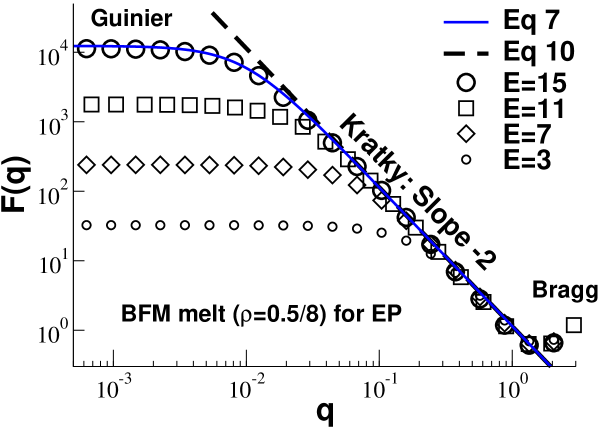
to extract the form factor (single chain scattering function) $F(q)$. To reveal the asymptotic behavior of the form factor for a Gaussian chain $F^{(0)}(q)\sim 12/q^{2}b^{2}$, one usually plots $q^{2}F({q})$ versus $q$ (called “Kratky plot”). The aim would be to show the existence of the “Kratky plateau” in the intermediate range of wave-vectors $\frac{2\pi}{\mbox{$R_{\text{g}}$}}\lesssim q\lesssim\frac{2\pi}{b}$ (“Kratky regime”) where $R_{\text{g}}$ is the radius of gyration of the macromolecule and $b$ is the (effective) statistical segment length doi1989 . In contrast to the low-$q$ “Guinier regime” ($q\lesssim\frac{2\pi}{\mbox{$R_{\text{g}}$}}$), clean scattering measurements can be performed in the Kratky regime footInhomogeneities suggesting the measurement of $b$ from the height of the Kratky plateau.

Surprisingly, this plateau appears to be experimentally elusive as already pointed out by Benoît BenBook : “Clearly, Kratky plots have to be interpreted with care“. For typical experiments, the available $q$-range is $5\cdot 10^{-3}/\text{\AA}<q<0.6/\text{\AA}$. Kratky plots are quickly increasing at high $q$ RawisoLectures ; BenBook , because of the rod-like effect starting at $q\sim\frac{1}{l_{\text{p}}}$, when the beam is scanning scales comparable with the persistence length $l_{\text{p}}$ (this regime is in fact used to assess $l_{\text{p}}$). Sometimes these curves can also quickly decrease, this is usually attributed to the fact that the chain cannot be considered as infinitely thin. The finite cross section of the chain tends to switch off the signal RawisoLectures ; BenBook as $\exp\left({-\frac{q^{2}R^{2}_{\text{c}}}{2}}\right)$, where $R_{\text{c}}$ is the radius of gyration of the cross section (in CS₂, a good solvent for dilute polystyrene, $R^{2}_{\text{c}}=9.5\text{\AA}^{2}$ MRRDCP1987 ). Rawiso et al. RawisoLectures ; BenBook have also shown that sometimes these two effects can compensate, for instance in a blend of hydrogenated and fully deuterated high molecular weight polystyrene, letting appear a pseudo Kratky plateau, extending outside the intermediate regime to higher $q$-values. In fact, taking for instance the case of polystyrene with $l_{\text{p}}\simeq 10\text{\AA}$, all these parasitic effects never really allowed neutron scattering experiments to confirm the Flory’s hypothesis. Up to now no scattering experiment has been performed on a sample allowing for a test over a wide enough range of $q$ footqrange ; Bates and there exists no clear experimental evidence of the Kratky plateau expected for Gaussian chains.

As we will show in this paper, there are fundamental reasons why this plateau may actually never be observed, even for samples containing very long and flexible polymers. Recently, long-range correlations, induced by fluctuations, have been theoretically derived ANSAJ2003 ; jojoPRL ; ANSSO2005 ; SOANSPRL2005 ; papEPL ; BeckrichThesis and numerically tested for two cavallowittmer and three-dimensional jojoPRL ; papEPL dense polymer systems. (Similar deviations from Flory’s ideality hypothesis have been also reported in various recent numerical studies on polymer melts CSGK91 ; Auhl03 and networks Sommer05 ; SGE05 .) The conceptually simpler part of these effects is related to the correlation hole scalingPGG and happens to dominate the non-Gaussian deviations to the form factor described here footMFcycles .

This is derived in the following Section II. There we first recapitulate the general perturbation approach (Sec. II.1), discuss then the intramolecular correlations in Flory size-distributed polymers (Sec. II.2). We obtain the form factor of monodisperse polymer melts by inverse Laplace transformation of the polydisperse case (Sec. II.3). In Section III these analytical predictions are illustrated numerically by Monte Carlo simulation of the three dimensional bond-fluctuation model BFM ; BWM04 . We compare melts containing only monodisperse chains jojoPRL ; papEPL with systems of (linear) equilibrium polymers (EP) CC90 ; WMC98 ; HXCWR06 where the self-assembled chains (no closed loops being allowed) have an annealed size-distribution of (essentially) Flory type footquench2anneal . Excellent parameter free agreement between numerical data and theory is demonstrated, especially for long EP (Sec. III.2). Finite-chain size effects are addressed as well. In the final Section IV the experimental situation is reconsidered in the light of our analytical and computational results. There we show numerically that eq 1 remains an accurate method for determining the form factor which should allow to detect the long-range correlations experimentally.

II Analytical Results

II.1 The Mean-Field Approach

It is well accepted that at the mean-field level doi1989 , the excluded volume interaction is entropically screened in dense polymeric melts. Long ago Edwards and de Gennes doi1989 ; scalingPGG ; RPAEd1 ; RPAEd2 ; cloiz developed a self-consistent mean-field method to derive a screened mean (molecular) field: this theory is an adaptation of the Random Phase Approximation (RPA) Nozieres to polymeric melts and solutions. The famous result of this approximation gives the response function $S(q)$ as a function of $F^{(0)}(q)$, the scattering function of a Gaussian (phantom) chain via the relation:

$$\frac{1}{S(q)}=\frac{1}{\rho F^{(0)}(q)}+v,$$ (2)

where $\rho$ is the mean concentration of monomers in the system and $v$ is the bare excluded volume (proportional to the inverse of the compressibility of the system). Please note that $F^{(0)}(q)$ has to be properly averaged over the relevant size-distribution of the chains cloiz . To get the effective interaction potential between monomers, we label a few chains. The interactions between labeled monomers are screened by the background of unlabeled monomers. Linear response gives the effective $q$ dependent excluded volume:

$$\frac{1}{\mbox{$v_{\text{eff}}$}(q)}=\frac{1}{v}+\rho F^{(0)}(q).$$ (3)

Let us from now on consider a dense system of long chains with exponentially decaying number density $\rho_{N}=\rho\mu^{2}e^{-\mu N}$ for polymer chains of length $N$ with $\mu\equiv 1/\mbox{$\left<N\right>$}$ being the chemical potential. This so-called Flory distribution is relevant to EP systems CC90 ; WMC98 . Hence, eq 3 yields (using eqs 6,7 indicated below)

$$\mbox{$v_{\text{eff}}$}(q)\hskip 2.84544pt\underset{R_{\text{g}}\gg\xi}{\approx}\hskip 2.84544pt\frac{v\xi^{2}}{1+q^{2}\xi^{2}}(q^{2}+\frac{\mu}{a^{2}}).$$ (4)

Here $a$ is the characteristic length of the monomer ($a^{2}\equiv{b^{2}}/{6}$) and $\xi=\sqrt{\frac{a^{2}}{2\rho v}}$ is the mean-field correlation length. When chains are infinitely long ($\mu\rightarrow 0$) we recover the classical result by Edwards doi1989 ignoring finite-size effects. If we further restrict ourselves to length scales larger than $\xi$ ($q\xi\ll 1$) eq 4 simplifies to $\mbox{$v_{\text{eff}}$}(q)\approx q^{2}a^{2}/2\rho$ which does not depend on the bare excluded volume $v$ and corresponds to the incompressible melt limit. For very large scales ($q\mbox{$R_{\text{g}}$}\ll 1$) one obtains the contact interaction associated to the volume $v^{*}\equiv\mbox{$v_{\text{eff}}$}(q\rightarrow 0)$, such that $v^{*}/v=\mu\xi^{2}/a^{2}\sim\xi^{2}/R_{\text{g}}^{2}$ (far weaker than the initial one given in the direct space by $v({\bf r})=v\delta({\bf r})$). The interaction $v^{*}$ is relevant to the swelling of a long chain immersed in the polydisperse bath scalingPGG .

The screened excluded volume interaction eq 4 taken at scale $R_{\text{g}}$ is weak and decays with chain length as $1/\mbox{$\left<N\right>$}$. The associated perturbation parameter $u$ in $d$-dimensional space depends on chain length as $u\sim v^{*}N^{2}/R_{\text{g}}^{d}\sim\mbox{$\left<N\right>$}^{1-d/2}$ and the screened excluded volume potential is, hence, perturbative in three dimensions scalingPGG .

Let us define $G({\bf q},s)=\langle\exp(-i{\bf q\cdot r}_{s})\rangle$, the Fourier transform of the two-point intramolecular correlation function, with $s=\arrowvert i-j\arrowvert$, the number of monomers between the two positions separated by ${\bf r}_{s}$. One can perturb the two-point Gaussian correlation function

$$G^{(0)}({\bf q},s)=\langle\exp(-i{\bf q\cdot r}_{s})\rangle_{0}=\exp{(-sq^{2}a^{2})}$$ (5)

with the molecular field eq 4. In this type of calculations, there are only three non-zero contributions ON83 ; Duplantier86 . They are illustrated by the diagrams given in Figure 1(a). Knowing this correlation, it is possible to derive many single-molecule properties BeckrichThesis .

Figure 1: (a) Interaction diagrams and (b) integration contour and singularities. (a) There exist three non-zero contributions to first-order perturbation, the first involving two points inside the segment of size $s=\arrowvert i-j\arrowvert$ monomers, the second involving one point inside and one outside the segment and the third involving one point on either side of the segment. Momentum $q$ flows from one correlated point to the other. Integrals are preformed over the momentum $k$. Dotted lines denote the effective interactions $v_{eff}(k)$, bold lines the propagators. (b) A possible contour in the complex plane. The dashed line depicts the logarithmic branch-cut, which is an arc of the circle of radius $r=\sqrt{\mu+q^{2}a^{2}}$ between $q_{1}=re^{i(\pi-\alpha)}$ and $q_{2}=re^{i\alpha}$, with $\alpha=\arctan(\sqrt{\mu/q^{2}a^{2}})$. The other singularities are single poles at $k=i\xi^{-1}$, $k=i\sqrt{\mu/a^{2}}$ and at $k=i\sqrt{q^{2}+\mu/a^{2}}$.

II.2 Intramolecular correlations for Flory size-distributed polymers

The intramolecular correlation function is investigated through its Fourier transform, the form factor. As already mentioned, we consider Flory size-distributed polymer systems footquench2anneal . In this case, one can define the form factor as:

$$F({q})=\sum_{N=0}^{\infty}\mu^{2}\exp(-\mu N)\sum_{i=1}^{N}\sum_{j=1}^{N}\langle\exp(-i{\bf q\cdot r}_{i,j})\rangle$$ (6)

with ${\bf q}$ the scattering vector. If the chains followed Gaussian statistics (as suggested by the Flory’s hypothesis), one should find using eq 5:

$$F^{(0)}({q})=\frac{2}{\mu}\ \frac{1}{1+q^{2}a^{2}/\mu}.$$ (7)

The ideal chain form factor for Flory size-distributed polymers is represented in the Figures 2, 3 and 4 where it is compared to our computational results on EP discussed below in Section III. In the small-$q$ regime, $qR_{\text{g}}\ll 1$ and for a polydisperse system, we can measure $R_{\text{g}}$ via the Guinier relation khokhlov+grosberg ; cloiz ; BenBook :

$$F({q})\hskip 1.42271pt\underset{qR^{(0)}_{\text{g}}\ll 1}{\simeq}\hskip 1.42271pt\frac{\langle N^{2}\rangle}{\mbox{$\left<N\right>$}}\left(1-\frac{q^{2}R_{\text{g,Z}}^{(0)\hskip 1.42271pt2}}{3}\right).$$ (8)

Please note the Z-averaging cloiz in the definition of $R_{\text{g,Z}}$

$$R_{\text{g,Z}}^{2}=\frac{\sum_{N}N^{2}\rho_{N}{R^{2}_{\text{g}}(N)}}{\sum_{N}N^{2}\rho_{N}},$$ (9)

$R_{\text{g}}(N)$ being the radius of gyration in the monodisperse case. (Since only Z-averaged length scales are considered below the index Z is dropped from now on.) As the Flory distribution gives $\langle N^{p}\rangle=\Gamma(p+1)/\mu^{p}$, one has ${R_{\text{g}}^{(0)\hskip 1.42271pt2}}={3a^{2}}/{\mu}$. In the Kratky regime between coil and monomer size one recovers the classical result for infinite chains

$$F^{(0)}({q})\hskip 1.42271pt\underset{qR^{(0)}_{\text{g}}\gg 1}{\simeq}\hskip 1.42271pt\frac{2}{q^{2}a^{2}},$$ (10)

(indicated by the dashed line in Figure 2) which expresses the fractal dimension of the Gaussian coil.

Figure 2: The intramolecular form factor $F(q)$ of polymer chains is an important property since it allows to make a connection between theory and simulation on the one hand and experiments of real systems on the other hand. The ideal chain form factor for Flory size-distributed polymers, eq 7, is indicated by the solid line. In the Kratky regime between the total chain and monomer sizes the form factor expresses the fractal dimension of the Gaussian coil, eq 10 (dashed line). Experimentally, this is the most important regime since it is, for instance, not affected by the (a priori unknown) polydispersity. The form factors of equilibrium polymers (EP) of various scission energies $E$ obtained numerically are indicated. The form factor of polydisperse polymer systems is obtained by computing for each chain $(\sum_{i}\sin({\bf q\cdot r}_{i}))^{2}+(\sum_{i}\cos({\bf q\cdot r}_{i}))^{2}$, summing over all chains (irrespective of their length) and dividing by the total number of particles. The computational data reveal an additional regime at wavevectors corresponding to the monomer structure (“Bragg regime”) which is not treated by our theory. All data have been obtained for a number density $\rho=0.5/8$ of the three dimensional bond-fluctuation model (BFM).

Perturbing the Gaussian correlation function with the screened potential $\mbox{$v_{\text{eff}}$}({\bf r})=\int\mbox{$v_{\text{eff}}$}(q)e^{i{\bf q\cdot r}}d^{3}{\bf q}/(2\pi)^{3}$, one has to evaluate $\left<\delta{\cal A}\right>=-\left<U{\cal A}\right>_{0}+\left<U\right>_{0}\left<{\cal A}\right>_{0}$ with $U=\frac{1}{2}\sum_{i,j}\mbox{$v_{\text{eff}}$}(r_{i}-r_{j})$ for the observable ${\cal A}$ of interest doi1989 . In our case, $\cal A$ corresponds the form factor, eq 6 (without average). The calculation in reciprocal space is schematically illustrated by the three diagrams given in Fig. 1(a) where bold lines represent propagators and dotted lines the effective interactions $\mbox{$v_{\text{eff}}$}({\bf k})$. For the first perturbation contribution, $\left<UF\right>_{0}$, the propagator carrying a momentum ${\bf p}$ (with ${\bf p}={\bf q}$ or ${\bf p}={\bf q}-{\bf k}$ as indicated in the diagrams) corresponds to a factor $1/(p^{2}a^{2}+\mu)$. For the second contribution, $\left<U\right>_{0}\left<F\right>_{0}$, the same rules apply but ${\bf q}$ has to be replaced by zero and (then) $\mu$ by $\mu+q^{2}a^{2}$. The momentum ${\bf k}$ is integrated out. Each diagram gives a converging contribution. Summing up the contributions of the diagrams (the central one has to be counted twice) and performing the angular integral (over the angle between ${\bf k}$ and ${\bf q}$) we arrive at the following integral:

$$\begin{split}\delta&F({q})=F({q})-F^{(0)}({q})=\\ &\frac{v}{4\pi^{2}a^{2}(\mu+q^{2}a^{2})^{2}}\int_{\mathbb{R}}dk\frac{k^{2}\xi^{2}}{1+k^{2}\xi^{2}}\hskip 2.84544pt\frac{(2\mu+(q^{2}+k^{2})a^{2})^{2}}{\mu+k^{2}a^{2}}\\ &\left(\frac{2}{\mu+(q^{2}+k^{2})a^{2}}-\frac{1}{2kqa^{2}}\ln\left(\frac{\mu+(q+k)^{2}a^{2}}{\mu+(q-k)^{2}a^{2}}\right)\right).\end{split}$$ (11)

The contributions to this integral come from two poles, one at $k=i\xi^{-1}$, this high-$k$ contribution renormalizes the statistical segment, and one at $k=i\sqrt{q^{2}+\frac{\mu}{a^{2}}}$, and from the logarithmic branch cut. The integration contour and the singularities are illustrated in Figure 1(b). Absorbing the high-$k$ pole contributions in the renormalized statistical segment $b^{*}$ doi1989 , and using $b^{*}$ instead of $b$ in the definition of $F^{(0)}({q})$, one finds (in the limit $q\xi<1$) as a function of $Q=q\mbox{$R^{(0)}_{\text{g}}$}=3qa^{2}/\mu$

$$\delta F(Q)/c=\frac{\sqrt{3}}{Q^{2}}\left(\frac{1}{(1+\frac{Q^{2}}{3})^{3/2}}-1\right)-\frac{1}{Q}\arctan\left(\frac{Q}{2\sqrt{3}}\right)+\frac{1}{\sqrt{3}}\frac{2+Q^{2}}{(1+\frac{Q^{2}}{3})^{2}}.$$ (12)

We have introduced here the factor $c=\frac{9\mbox{$R^{(0)}_{\text{g}}$}}{\pi\rho\mbox{$b^{*}$}^{4}}$ to write the deviation in a form which should scale with respect to chain length. The statistical segment length $b^{*}$, we have introduced, is given by

$$\mbox{$b^{*}$}^{2}=b^{2}\hskip 1.42271pt\left(1+\frac{12v\xi}{\pi b^{4}}\right).$$ (13)

which is consistent with the result obtained by Edwards and Muthukumar E75 ; ME82 ; doi1989 .

Figure 3: Successful scaling of the form factors of EP obtained from our BFM simulations for various scission energies $E$ as indicated: $F(Q)/F(0)$ is plotted vs. the reduced wavevector $Q=\mbox{$R_{\text{g}}$}q$. Note that both scales $F(Q\rightarrow 0)=\left<N^{2}\right>/\mbox{$\left<N\right>$}$ and the (Z-averaged) gyration radius $R_{\text{g}}$ have been directly measured for each sample and are indicated in Table 1. Obviously, the scaling breaks down due to local physics for large wavevectors (Bragg regime). The line represents the prediction for ideal Flory-distributed polymers, eq 7, with parameters chosen in agreement with the Guinier limit, eq 8. Importantly, in the intermediate Kratky regime small, albeit systematic, deviations are visible which will be further investigated below.

Figure 4: Kratky representation of the intramolecular form factor $F(q)q^{2}$ vs. wavevector $q$ for monodisperse (crosses) and equilibrium polymers. The non-monotonous behavior predicted by the theory is clearly demonstrated. The ideal chain form factor, eq 7 (thin line), overpredicts the dip of the form factor at $q\approx 0.7$ by about $20\%$. The bold line indicates the prediction for infinite chains, eq 23, which should hold for both system classes for infinitely long chains. For this reason we have chosen the largest chains currently available.

Figure 5: Correction $\delta F(Q)=F(Q)-F^{(0)}(Q)$ to the form factor as a function of $Q=q\mbox{$R^{(0)}_{\text{g}}$}$ (using $\mbox{$R^{(0)}_{\text{g}}$}^{2}=3\mbox{$a^{*}$}^{2}/\mu$) as predicted by eq 12 for Flory-distributed polymers. The deviation is positive for small wavevectors (Guinier regime) and becomes negative at about $Q\approx 3$. The scaling factor $c=9\mbox{$R^{(0)}_{\text{g}}$}/\pi\rho\mbox{$b^{*}$}^{4}$ should allow a data collapse irrespective of the mean chain size — provided that the chains are sufficiently long to suppress additional physics in the Bragg regime. Also included are eq 14 and 18 for the asymptotic behavior in the Guinier and the Kratky regimes respectively. The data from our BFM simulations (given here for two scission energies where high precision data are available) agree quantitatively (especially for small $Q$) with eq 12. (Note that the chains are too short to allow a better fit for large $Q$.) The reference form factor $F^{(0)}(Q)$ has been computed from eq 7 supposing a perfect Flory distribution.

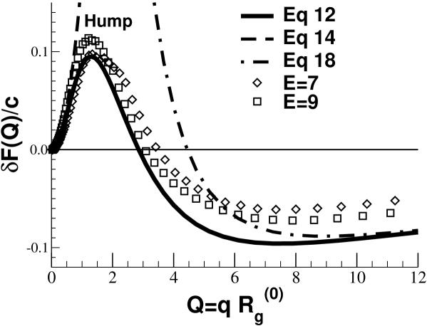
As may be seen from the plot of eq 12 in Figure 5 the deviation from ideality is positive for small wave-vectors (with a pronounced maximum at $Q\approx 1$). It becomes negative when the internal coil structure is probed ($Q\gg 2$). Asymptotically, eq 12 gives

$$\delta F(q)\underset{\frac{qa}{\sqrt{\mu}}\ll 1}{\simeq}\frac{11R^{(0)}_{\text{g}}}{4\sqrt{3}\pi\rho\hskip 1.42271pt\mbox{$b^{*}$}^{4}}q^{2}{R^{(0)\hskip 1.42271pt2}_{\text{g}}},$$ (14)

(dashed line in Figure 5) which highlights the average swelling factor of the molecule in the melt:

$$R^{2}_{\text{g}}={R^{(0)2}_{\text{g}}}\hskip 1.42271pt\frac{\mbox{$b^{*}$}^{2}}{b^{2}}\left(1-\frac{11\sqrt{6}}{16\pi\rho\hskip 1.42271pt\mbox{$b^{*}$}^{3}}{\sqrt{\mu}}\right)$$ (15)

(comparable to a logarithmic term in the two-dimensional case ANSAJ2003 ; NO81 ). This is a sign of swelling, because $R_{\text{g}}=\langle N\rangle^{1/2}f(\sqrt{\langle N\rangle})$, with $f$, an increasing function, showing that the apparent swelling exponent $\nu$ for finite $\left<N\right>$ is slightly larger than $1/2$. It is interesting to compare it with the (also Z-averaged) end-to-end distance, easily available because it involves only the top-left diagram of Figure 1:

$$R_{\text{e}}^{2}={R^{(0)2}_{\text{e}}}\hskip 1.42271pt\frac{\mbox{$b^{*}$}^{2}}{b^{2}}\left(1-\frac{10\sqrt{6}}{16\hskip 1.42271pt\pi\rho\hskip 1.42271pt\mbox{$b^{*}$}^{3}}\sqrt{\mu}\right).$$ (16)

(The diagram must be twice differentiated with respect to $\bf{q}$.) The naively defined size dependent effective statistical segment of an $N$-chain (from $R_{\text{e}}^{2}=b^{2}_{\text{eff}}N$) therefore is:

$$b^{2}_{\text{eff}}=\mbox{$b^{*}$}^{2}\left(1-\frac{\mbox{const}}{\rho\hskip 1.42271pt\mbox{$b^{*}$}^{3}\sqrt{N}}\right)$$ (17)

The size-dependences in eqs 15,16 follow the same scaling, but the numerical factors are different. Although internal segments carry a smaller correction jojoPRL , the size-dependent contact potential $\mu/2\rho$ in eq. 4 counterbalances this effect and makes the correction to eq 16 a little smaller than the one in eq 15.

The asymptotic behavior of eq 12 in the Kratky regime gives

$$\delta F(q)\underset{qR_{\text{g}}\gg 1}{\simeq}\frac{12}{q^{2}\mbox{$b^{*}$}^{2}}\left(\frac{3\sqrt{6}}{\pi\rho\hskip 1.42271pt\mbox{$b^{*}$}^{3}}\sqrt{\mu}-\frac{3q}{8\rho\hskip 1.42271pt\mbox{$b^{*}$}^{2}}\right),$$ (18)

which is represented in Figure 5 by the dashed-dotted line. The first term in this equation is a size-dependent shift of the Kratky plateau, and the second one, independent of the size, makes the essential difference with the Flory prediction (bold line in Figure 4). Hence, the corrections induced by the screened potential are non-monotonic (Figure 5).

Eq 11 is not restricted to $q\xi<1$, it is applicable over the entire $q$-range in the case of weakly fluctuating dense polymers footcumbersome (mean-field excluded volume regime) as may be simulated with soft monomers allowed to overlap with some small penalty. In the case of strong excluded volume and less dense solutions (critical semidilute regime, not explicitly considered here) the results are valid at scales larger than $\xi$ provided the statistical segment is properly renormalized. Quantitatively, the Ginzburg parameter measuring the importance of density fluctuations reads $G_{z}^{2}=v/(\rho\hskip 1.42271ptb^{6})$. For persistent chains $l_{\text{p}}>t$, $t$ being the thickness of the chain, density fluctuations are negligible provided $G_{z}^{2}\sim 1/(\tilde{\rho}\hskip 1.42271ptl_{\text{p}}^{3}/t^{3})\ll 1$, with $\tilde{\rho}=\rho\hskip 1.42271ptt^{3}$, the monomer volume fraction. The above makes sense if $\xi\gg l_{\text{p}}$, which requires $\tilde{\rho}<t/l_{p}$. This criterion also indicates the isotropic/nematic transition khokhlov+grosberg ; LiqCrysSem . In summary, mean-field applies provided $\left(\frac{t}{l_{\text{p}}}\right)^{3}<\tilde{\rho}<\frac{t}{l_{\text{p}}}$.

II.3 Monodisperse polymer melts in three dimensions

It is possible to relate the form factor of the polydisperse system (Flory distribution) to the form factor $F_{N}({q})$ of a monodisperse system. Following eq 6,

$$F(q)=\frac{\sum_{N=0}^{\infty}\rho_{N}NF_{N}({q})}{\sum_{N=0}^{\infty}\rho_{N}N}=\sum_{N=0}^{\infty}\mu^{2}\exp(-\mu N)NF_{N}({q})$$ (19)

the deviations of the form factors of monodisperse and polydisperse systems are related by the inverse Laplace transformation $\delta F_{N}({q})=\frac{1}{N}\mathcal{L}^{-1}\left(\frac{1}{\mu^{2}}\delta F(q)\right)$, $\mathcal{L}$ being the Laplace transform operator. Using our result eq 12 for polydisperse systems this yields:

$$\delta F_{N}(Q)/c \simeq \frac{2}{\sqrt{\pi}Q^{2}}e^{-Q^{2}}+\frac{5}{\sqrt{\pi}Q^{2}}-\left(\frac{2}{\sqrt{\pi}Q}+\frac{7}{\sqrt{\pi}Q^{3}}\right)D(Q)$$ (20)

$$+ \frac{4}{\sqrt{\pi}Q^{3}}\int_{0}^{1}\left(\frac{2}{\alpha^{3}}D\left(\frac{\alpha Q}{2}\right)-\frac{Q}{\alpha^{2}}\right)d\alpha,$$

where $Q=qR^{(0)}_{\text{g},N}$ with $R^{(0)}_{\text{g},N}=\sqrt{N}a$, the radius of gyration in the ideal monodisperse case and $D(x)$ is the Dawson function, whose definition is $D(x)=e^{-x^{2}}\int_{0}^{x}e^{t^{2}}dt$ abramowitz .

Figure 6: Deviation to the ideal form factor in a monodisperse system, eq 20. The shape is similar to that in the polydisperse case (Figure 5) since polydispersity merely affects the Guinier regime. Also indicated are the asymptotic behavior in the Kratky regime, eq 21, and the prediction for infinite chains, eq 22. The simulation data scales roughly, especially in the Guinier limit (hump), while for larger $q$ deviations are visible which may be attibuted to local physics. The agreement with eq 20 is only qualitative here since a much more proncounced non-monotonic behavior is seen in the simulation. This is due to use of the polydisperse chain perturbation potential, eq 4 — an approximation which must become insufficient for low wavevectors where the coil size matters.

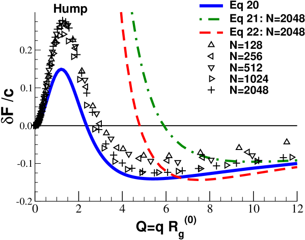
Eq 20, shown in Figure 6 (bold line), is accurate up to the finite size corrections to the interaction potential as these have been calculated for the Flory distribution, eq 4. However, on small length scales, this influence is weakened, and in this limit, it gives:

$$F(q)\underset{qR_{\text{g}}\gg 1}{\simeq}\frac{12}{q^{2}\mbox{$b^{*}$}^{2}}\left(1+\frac{6\sqrt{6}}{\pi^{3/2}\rho\hskip 1.42271pt\mbox{$b^{*}$}^{3}}\frac{1}{\sqrt{N}}-\frac{3q}{8\rho\mbox{$b^{*}$}^{2}}\right).$$ (21)

Eq 21 is represented in Figure 6 by the dashed-dotted line footPade . Taking $\langle N\rangle=1/\mu$, eq 18 deviates from eq 21 only by the numerical coefficient in front of $1/\sqrt{N}$. The difference is $\sim 10\%$.

II.4 Infinite chain limit and scaling arguments

It is worthwhile to discuss the infinite chain limit, $\mu\rightarrow 0$, that puts forward most clearly the essential differences with an ideal chain. (The differences between monodisperse and polydisperse systems are inessential in this limit.) We can write the form factor of an infinite chain ($R_{\text{g}}\rightarrow\infty$) at scales larger than $\xi$ as:

$$F({q})=\frac{12}{q^{2}\mbox{$b^{*}$}^{2}}\frac{1}{\left(1+\frac{3}{8}\frac{qb^{*}}{\rho\hskip 1.42271ptb^{*3}}\right)}.$$ (22)

Following standard notations cavallowittmer ; SchaferBook ; LSMMKB2000 , we may rewrite eq 22 in the form:

$$\frac{1}{F({q})}=\frac{q^{2}\mbox{$b^{*}$}^{2}}{12}+\frac{1}{32}\frac{q^{3}}{\rho}.$$ (23)

See the Figures 4 (bold line), 6 (dashed line) and 9 (bold line) for representations of this important limiting behavior. The correction term obtained in the one-loop approximation (eq 23) depends neither on the excluded volume parameter $v$ nor on the statistical segment. Hence, it is expected to hold even in the strongly fluctuating semidilute regime and it is of interest to compare our results with the recent renormalization group calculations of L. Schäfer SchaferBook . There the skeleton diagrams for the renormalization of interaction and statistical segment have also been performed within the one loop approximation. From the above it is expected that both results are identical. After careful insertions (eq 18.23, p. 389 of Ref. SchaferBook ) a $q^{3}/\rho$ correction can be extracted with the universal amplitude $0.03124..$. The fact that this numerical amplitude is so close to our $1/32=0.03125$ comforts both our and Schäfer’s result.

Performing an inverse Fourier transform of the form factor, eq 22 gives not only the Coulomb-like term from the singularity at the origin, but also another long-range contribution arising from the branch cut:

$$G_{\text{intra}}({r})=\frac{12}{\mbox{$b^{*}$}^{2}}\frac{1}{4\pi r}-\frac{9}{4}\frac{1}{\rho\mbox{$b^{*}$}^{4}}\frac{1}{\pi^{2}r^{2}}.$$ (24)

The correction is never dominant in real space. But both contributions are different in nature. In the collective structure factor ANSSO2005 ; SOANSPRL2005 $S^{-1}(q)\sim v+c_{2}q^{2}+c_{3}q^{3}$, the leading singularity of eq 22 is shifted away from the origin and the corresponding contribution is screened on the lengthscale $\xi$ in real space. The branch cut (from the $q^{3}$ term) still contributes a power law, namely an anticorrelation term decreasing as $r^{-6}$, that has been identified as a fluctuation-induced Anti-Casimir effect ANSSO2005 ; SOANSPRL2005 (or as the $n-1=-1$ Goldstone mode in the polymer-magnet analogy SO1990 ). The average number of particles from the same molecule in a sphere of radius $R$, $\mathcal{N}(R)=\int G_{\text{intra}}({r})d^{3}{\bf r}$ is decreased (compared to a Gaussian coil) because of the sign of the correction. Nevertheless, the differential (apparent) Hausdorff dimension Hausdorff $d_{\text{H}}$ as defined by $d_{\text{H}}={\text{d}}\log\mathcal{N}(R)/{\text{d}}\log R$ is increased.

The fluctuation corrections presented in eqs 22,23,24 can be interpreted with the following argument, involving $\tilde{G}(r,s)$, the correlation function of two points separated by $s$ monomers, $\tilde{G}(r,s)=\int G(q,s)e^{{\rm i}{\bf q}\cdot{\bf r}}\frac{{\rm d}^{3}q}{(2\pi)^{3}}$. For large $s$, the difference $\delta\tilde{G}(r,s)\equiv\tilde{G}(r,s)-\tilde{G}^{(0)}(r,s)$ is discussed below in the limit of large and small geometrical separation $r$ between monomers. Here $\tilde{G}^{(0)}(r,s)={\rm c}{\rm o}{\rm n}{\rm s}{\rm t}\,\,\exp\left(-\frac{3}{2}\frac{r^{2}}{s\mbox{$b^{*}$}^{2}}\right)$, where the renormalized $b^{*}$ is used instead of $b$.

A highly stretched $s$-fragment ($r\gg\mbox{$b^{*}$}\sqrt{s}$) can be viewed as a string of Pincus blobs, each blob of $g\sim s^{2}b^{2}/r^{2}$ units. Different blobs do not overlap in this limit, therefore the effective statistical segment of the blob, $b_{\text{eff}}$ comes as a result of interactions of units inside the blob (see eq 17)

$$b^{2}_{\text{eff}}=\mbox{$b^{*}$}^{2}\left(1-\frac{const}{\rho\hskip 1.42271pt\mbox{$b^{*}$}^{3}\sqrt{g}}\right)$$ (25)

where $const$ is a universal numerical constant. The elastic energy of stretching the $s$-segment is therefore

$$W_{el}(r)\simeq n_{b}\frac{3}{2}\frac{\left(r/n_{b}\right)^{2}}{gb_{\text{eff}}^{2}}=\frac{3}{2}\frac{r^{2}}{sb_{\text{eff}}^{2}}\simeq\frac{3}{2}\frac{r^{2}}{s\mbox{$b^{*}$}^{2}}\left(1+{\rm c}{\rm o}{\rm n}{\rm s}{\rm t}\,\frac{r}{\rho\mbox{$b^{*}$}^{4}s}\right)$$

where $n_{b}=s/g$ is the number of blobs in the $s$-segment. Thus, when $r\gg\sqrt{s}\mbox{$b^{*}$}$:

$$\tilde{G}(r,s)={\rm c}{\rm o}{\rm n}{\rm s}{\rm t}\,e^{-W_{el}(r)}\simeq\tilde{G}^{(0)}(r,s)\exp\left(-{\rm c}{\rm o}{\rm n}{\rm s}{\rm t}\,\frac{r^{3}}{\rho\hskip 1.42271pt\mbox{$b^{*}$}^{6}s^{2}}\right)$$ (26)

The faster decay of $\tilde{G}$ as compared to $\tilde{G}^{(0)}$ leads to higher scattering (positive $\delta F(q)$) at small $q$.

On smaller length scales, $r\ll\sqrt{s}\mbox{$b^{*}$}$, it is convenient to consider the $s$-fragment as a chain of blobs of size $r$, with $g\sim r^{2}/{\mbox{$b^{*}$}^{2}}$. This is sketched in Figure 7.

Figure 7: For small internal end-to-end distances ($r\ll\sqrt{s}\mbox{$b^{*}$}$), monomers of terminal blobs with $g\sim r^{2}/\mbox{$b^{*}$}^{2}$ units interact.

The correction $\delta\tilde{G}$ here is essentially due to the direct interaction of the overlapping blobs or radius $r$ around the two correlated monomers. The number of binary contacts is proportional to $g^{2}/r^{3}$, while the pairwise interaction between monomers scales like $1/(g\rho)$ (see eq 4), giving ANSAJ2003 $U\sim g/(\rho\hskip 1.42271ptr^{3})\sim 1/(r\mbox{$b^{*}$}^{2}\rho)$. Therefore, for $\xi\ll r\ll\sqrt{s}\hskip 1.42271pt\mbox{$b^{*}$}$,

$$\begin{split}\tilde{G}(r,s)&\simeq\tilde{G}^{(0)}(r,s)\left(1-U\right)\\ &\simeq\tilde{G}^{(0)}(r,s)\left(1-\frac{const}{r\mbox{$b^{*}$}^{2}\rho}\right),\end{split}$$ (27)

which qualitatively explains eq 24. For $q\gg\frac{1}{\sqrt{s}b}$, we get:

$$\delta G(q,s)=-const\left(\frac{6}{4\pi\mbox{$b^{*}$}^{2}s}\right)^{\frac{3}{2}}\frac{4\pi}{q^{2}\mbox{$b^{*}$}^{2}\rho}.$$ (28)

This regime is also limited by the condition $q\xi\ll 1$. Thus the low-$q$ correction is positive and it increases with $q$, while the high-$q$ correction $\delta G(q,s)$ is negative and is also increasing with $q$, implying an intermediate decline. This non-monotonic behavior of $\delta G(q,s)$ translates in a non-monotonic dependence of $\delta F(q)$ for finite $N$ (Figure 6).

To underline the origin of the ”non-analytical” term $1/q$, let us give some details of an easy calculation of the correction to the correlation function for the infinite chain. The top-left diagram in Figure 1 is the only diagram producing this term.

Figure 8: Diagram producing the non-analytical term for an infinite chain. The mixing of the wave-vectors is pinned in the (m,n) segment. The summation is done on (n,t) and (m,l).

With notations shown in Figure 8 we can write the corresponding analytical expression:

$$\begin{split}\delta&F(q)=-\underset{t-n}{\sum_{n-m,m-l}}\int{d{\bf k}}\hskip 1.42271pt\mbox{$v_{\text{eff}}$}({\bf k})\exp({-{\bf k}^{2}(m-l)a^{2}})\\ &\exp(-({\bf q}+{\bf k})^{2}(n-m)a^{2})\exp({-{\bf k}^{2}(n-t)a^{2}}).\end{split}$$ (29)

Here $e^{-{\bf k}^{2}(m-l)a^{2}}$ is the Gaussian (bare) correlation function of the chain between monomers $l$ and $m$. In the interaction, we will leave only the $k^{2}$-dependent part. After summation (integration) over $m-l$ and $n-t$ we get:

$$\delta F(q)=-\frac{v\xi^{2}}{a^{4}}\sum_{n-m=0}^{\infty}\int\exp({-({\bf q}+{\bf k})^{2}(m-n)a^{2}})d\cos(\theta)dk.$$ (30)

Then, after integration over $n-m$ we get:

$$\delta F(q)=-\frac{v\xi^{2}}{|q|a^{6}}\int_{-1}^{1}\frac{d\cos(\theta)}{\sqrt{1-\cos^{2}(\theta)}}\simeq-\frac{1}{\rho\mbox{$b^{*}$}^{3}}\frac{1}{|q|\mbox{$b^{*}$}}$$ (31)

which is similar to eq 28. It should be emphasized that for a finite chain, the finite summation over $m-l$ and $n-t$ produces extra terms, and these ”odd” terms exist only for $qR_{\text{g}}<1$.

III Computational results

The previous section contains non-trivial results due to generic physics which should apply to all polymer melts containing long and preferentially flexible chains. We have put these predictions to a test by means of extensive lattice Monte Carlo simulations BWM04 of linear polymer melts having either a quenched and monodisperse or an annealed size-distribution. For the latter “equilibrium polymers” (EP) one expects (from standard linear aggregation theory) a Flory distribution if the scission energy $E$ is constant (assuming especially chain length independence) CC90 ; WMC98 ; footquench2anneal . (Apart from this finite scission energy for EP all our systems are perfectly athermal. We set $k_{B}T=1$ and all length scales will be given below in units of the lattice constant.) We sketch first the algorithm used and the samples obtained and discuss then the intramolecular correlations as measured by computing the single chain form factor $F(q)$.

III.1 Algorithm and some technical details

For both system classes we compare data obtained with the three dimensional bond-fluctuation model (BFM) BFM where each monomer occupies the eight sites of a unit cell of a simple cubic lattice. For details concerning the BFM see Refs. BFM ; BWM04 ; WMC98 . For all configurations we use cubic periodic simulation boxes of linear size $L=256$ containing $2^{20}$ monomers. These large systems are needed to suppress finite size effects, especially for EP WMC98 . The monomer number relates to a number density $\rho=1/16$ where half of the lattice sites are occupied (volume fraction $0.5$). It has been shown that this “melt density” is characterized by a small excluded volume correlation length $\xi$ of order of the monomer size BFM ; BWM04 , by a low (dimensionless) compressibility, $S(q\rightarrow 0)/\rho=1/v\rho=0.24$, as may be seen from the bold line ($f=1$) indicated in the main panel of Figure 10 below, and an effective statistical segment length, $\mbox{$b^{*}$}\approx 3.24$ jojoPRL ; footbstar .

The chain monomers are connected by (at most two saturated) bonds. Adjacent monomers are permanently linked together for monodisperse systems (if only local moves through phase space are considered). Equilibrium polymers on the other hand have a finite and constant scission energy $E$ attributed to each bond (independent of density, chain length and position of the bond) which has to be paid whenever the bond between two monomers is broken. Standard Metropolis Monte Carlo is used to break and recombine the chains. Branching and formation of closed rings are explicitly forbidden and only linear chains are present. The delicate question of “detailed balance”, i.e. microscopic reversibility, of the scission-recombination step is dealt with in Ref. HXCWR06 .

The monodisperse systems have been equilibrated and sampled using a mix of local, slithering snake and double pivot moves extending our previous studies jojoPRL ; papEPL . This allowed us to generate ensembles containing about $10^{3}$ independent configurations with chain length up to $N=8192$ monomers. More information on equilibration and sample characterization will be given elsewhere papRsPs . We have sampled EP systems with scission energies up to $E=15$, the largest energy corresponding to a mean chain length $\mbox{$\left<N\right>$}\approx 6000$. Some relevant properties obtained for these EP systems are summarized in Table 1. It has been verified (as shown in Refs. WMC98 ; HXCWR06 ) that the size-distribution obtained by our EP systems is indeed close to the Flory distribution studied in the analytical approach presented in the previous section. For EP only local hopping moves are needed in order to sample independent configurations since the breaking and recombination of chains reduce the relaxation times dramatically, at least for large scission-recombination attempt frequencies footequilibrate . In fact, all EP systems presented here have been sampled within four months while the sample of monodisperse $N=8192$ configurations alone required about three years on the same XEON processor. EP are therefore very interesting from the computational point of view, allowing for an efficient test of theoretical predictions which also apply to monodisperse systems.

III.2 Form factor

It is well known that the intramolecular single chain form factor of monodisperse polymer chains may be computed using

$$F_{N}(q)\equiv\frac{1}{N}\left<\left(\sum_{i=1}^{N}\cos({\bf q\cdot r}_{i})\right)^{2}+\left(\sum_{i=1}^{N}\sin({\bf q\cdot r}_{i})\right)^{2}\right>,$$ (32)

the average being taken over all chains and configurations available. The form factor obtained for the largest available monodisperse chain systems currently available is represented in the Figures 4, 6, 7 and 9. It should be emphasized that the correct generalization of eq 32 to polydisperse systems compatible with eqs 6 and 19 is the average with weight $N\rho_{N}$ over $F_{N}(q)$. In practice, one computes simply the ensemble averaged sum over $(\sum_{i=1}^{N}\sin({\bf q\cdot r}_{i}))^{2}+(\sum_{i=1}^{N}\cos({\bf q\cdot r}_{i}))^{2}$ contributions for each chain and divides by the total number of monomers.

Figure 2 presents the (unscaled) form factors obtained for four different scission energies for our BFM EP model at $\rho=1/16$. The three different $q$-regimes are indicated. Details of the size-distribution must matter most in the Guinier regime which probes the total coil size. Non-universal contributations to the form factor arise at large wavevectors (Bragg regime). Obviously, the larger $E$ the wider the intermediate Kratky regime (see the dashed line indicating eq 10) where chain length, polydispersity and local physics should not contribute much to the deviations of the form factor from ideality. A very similar plot (not shown) has been obtained for monodisperse polymers. Not surprisingly, it demonstrates that the form factors of both system classes become indistinguishable for large wavevectors.

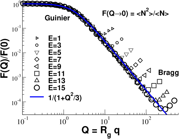
The natural scaling attempt for the form factor of EP is presented in Figure 3 for a broad range of scission energies. We plot $F(Q)/F(0)$ as a function of $Q=q\mbox{$R_{\text{g}}$}$ where both $F(q\rightarrow 0)=\left<N^{2}\right>/\mbox{$\left<N\right>$}$ and the (Z-averaged) gyration radius $R_{\text{g}}$ have been measured directly for each $E$. Note that the strong variation of $F(0)$ and $R_{\text{g}}$ with $E$ showing that the successful scaling collapse is significant. Obviously, this scaling does not hold in the Bragg regime ($q\approx 1$) where $F(q)$ increases rapidly, as one expects. The bold line represents the ideal chain form factor, eq 7, where the identification of the coefficients, $F(0)\rightarrow 2/\mu$ and $\mbox{$R_{\text{g}}$}^{2}\rightarrow 3a^{2}/\mu$, is suggested by the Guinier limit, eq 8. Hence, the perfect fit for $q\ll 1/\mbox{$R_{\text{g}}$}$ is imposed, but the agreement remains nice even for much larger wavevectors. A careful inspection of the Figure reveals, however, that eq 7 overestimates systematically the data in the Kratky regime. (The corresponding plot for monodisperse chains is again very similar.)

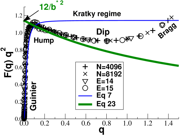
This can be seen more clearly in the Kratky representation given in Figure 4 in linear coordinates. We present here the systems with the longest masses currently available for both monodisperse ($N=4096$ and $N=8192$) and EP systems ($E=14$ and $E=15$). The non-monotonous behavior is in striking conflict with Flory’s hypothesis. The difference between the ideal Gaussian behavior (thin line) and the data becomes up to 20%. For the large (average) chain masses given here all systems are identical for $q\geq 0.1$ (but obviously not on larger scales). It should be noted that qualitatively similar results have been reported — albeit for much shorter chains — for more than a decade in the literature CSGK91 ; LSMMKB2000 . The infinite chain prediction, eq 23 (or equivalently eq 22), gives a lower envelope for the data which fits reasonably — despite its simplicity — in the finite wavevector range $0.1<q<0.4$.

The form factor difference $\delta F(q)=F(q)-F^{(0)}(q)$ is further investigated in the Figures 5 and 6 for equilibrium and monodisperse systems respectively. These plots highlight the deviations in the Guinier regime. In both cases the ideal chain form factor $F^{(0)}(q)$ is computed assuming the same effective statistical segment length $\mbox{$b^{*}$}=\mbox{$a^{*}$}\sqrt{6}$, i.e. the reference chain size is $\mbox{$R^{(0)}_{\text{g}}$}=\mbox{$a^{*}$}N^{1/2}$. In the first case the reference $F^{(0)}(q)$ is the ideal chain form factor for Flory-distributed chains, eq 7, in the second the Debye function $F^{(0}(q)=Nf_{D}(Q^{2})$ with $f_{D}(x)=(\exp(-x)-1+x)2/x^{2}$ doi1989 .

As suggested by eq 12 and eq 20 respectively we plot $\delta F(q)/c$ vs. $Q=q\mbox{$R^{(0)}_{\text{g}}$}$, i.e. the axes have been chosen such that the data should scale for different (mean) chain length. We obtain indeed a reasonable scaling considering that our chains are not large enough to suppress (for the $Q$-range represented) the deviations $\delta F(q)$ due to local physics. The scaling shows implicitly that the corrections with respect to the infinite chain limit decay as the inverse gyration radius, $1/c\sim 1/\sqrt{N}$, as predicted by eqs 18 and 21. (Both plots appear to improve systematically with increasing chain length and, clearly, high precision form factors for much larger chains must be considered in future studies to demonstrate the scaling numerically.) Also the functional agreement with theory is qualitatively satisfactory in both cases, for equilibrium polymers it is even quantitative for small wavevectors. For monodisperse chains we find numerically a much more pronounced hump in the Guinier as the one predicted by eq 20 (bold). This is very likely due to the chosen interaction potential eq 4 for Flory-distributed chains which is not accurate enough for the description of the Guinier regime of monodisperse chains.

It should be pointed out that the success of the representation of the non-Gaussian deviations chosen in the Figures 5 and 6 does depend strongly on the accurate estimation of the statistical segment length $b^{*}$ of the ideal reference chains. A variation of a few percents breaks the scaling and leads to qualitatively different curves. Since such a precision is normally not available (neither in simulation nor in experiment) it is interesting to find a more robust representation of the form factor deviations which does not rely on $b^{*}$ and allows to detect the theoretical key predictions for long chains (notably eq 23) more readily.

Figure 9: Scaling attempt of the non-Gaussian deviations of the form factor of monodisperse polymers in the melt in terms of the measured radius of gyration $R_{\text{g}}$ (instead of $R^{(0)}_{\text{g}}$). As suggested by eq 23, the difference $1/F(q)-1/F^{(0)}(q)$ of the measured and the ideal chain Debye form factor has been rescaled by the factor $N\rho/\mbox{$\rho^{*}$}$ and plotted as a function of $Q=q\mbox{$R_{\text{g}}$}$. We obtain perfect data collapse for all chain lengths included. (Obviously, data points in the Bragg limit $q\approx 1$ do not scale.) The difference $-\delta F(q)$ is positive in all regimes and no change of sign occurs in this representation. Note that the power law slope, $m(Q)=Q^{3}/32$, predicted by eq 23, can be seen over more then one order of magnitude. In the Guinier regime, the difference increases more rapidly, $m(Q)\propto Q^{4}$ (dashed line), as one expects from a standard analytic expansion in $Q^{2}$.

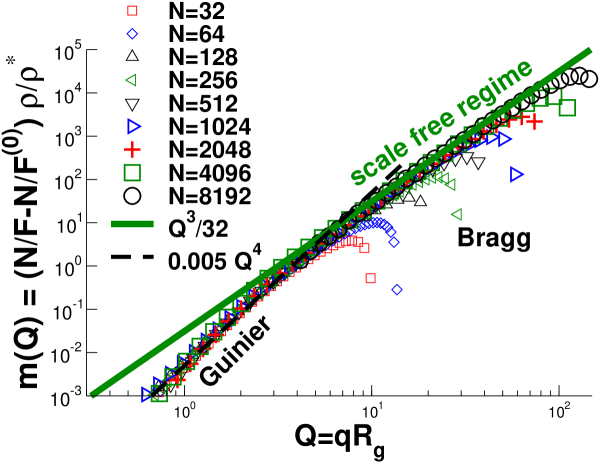
Such a representation is given in Figure 9 for monodisperse chains. (A virtually indistinguishable plot has been obtained for EP.) The reference chain size is set here by the measured radius of gyration $\mbox{$R_{\text{g}}$}(N)$ (replacing the above $R^{(0)}_{\text{g}}$) which is used for rescaling the axis and, more importantly, to compute the Debye function $F^{(0)}(q)$. The general scaling idea is motivated by Figure 3, the scaling of the vertical axis is suggested by eq 23 which predicts the difference of the inverse form factors to be proportional to $N^{0}q^{3}$. Without additional parameters ($R_{\text{g}}$ is known to high precision) we confirm the scaling of

$$m(Q)\equiv\left(\frac{N}{F(q)}-\frac{N}{F^{(0)}(q)}\right)\rho/\mbox{$\rho^{*}$}$$ (33)

as a function of $Q=q\mbox{$R_{\text{g}}$}$ with $\mbox{$\rho^{*}$}\equiv N/\mbox{$R_{\text{g}}$}^{3}$ being the overlap density. Importantly, our simulations allow us to verify for $Q\gg 5$ the fundamentally novel $Q^{3}$ behavior of the master curve predicted by eq 23 and this over more than an order of magnitude!

Figure 10: The response function $S(q,f)$ of a fraction $f$ of marked monodisperse chains of chain length $N=512$. The remaining $1-f$ chains are considered to be not “visible” for the scattering. (The simulation box of linear size $L=256$ contains 2048 chains in total.) The main figure (a) presents $S(q,f)$ directly as computed from $S(q,f)/\rho f=\frac{1}{n}\left<\left(\sum_{i}\cos({\bf q\cdot r}_{i})\right)^{2}+\left(\sum_{i}\sin({\bf q\cdot r}_{i})\right)^{2}\right>$ where the sums run over all $n=L^{3}\rho f$ marked monomers and the wavevectors are commensurate with the cubic box. Also included is the form factor $F(q)$ (dashed line) from eq 32 which corresponds to the $S(q,f)/\rho f\stackrel{{\scriptstyle f\rightarrow 0}}{{\Rightarrow}}F(q)$ limit (but compares already perfectly with the $f=0.01$ data set). The so-called “total structure factor” $S(q,f=1)$ (bold line at bottom) is the Fourier transformed monomer pair-correlation function of all monomers. For scales larger than the monomer size it is essentially constant and yields an accurate determination of the (dimensionless) compressibility $S(q)/\rho=1/v\rho\approx 0.24$. Since the compressibility is finite, although small, this value has to be properly taken into account if one wants to estimate the form factor $F(q)$ from the experimentally available $S(q,f)$. The inset (b) presents a Kratky representation of $S(q,f)$ as suggested by an appropriate generalization of eq 1: $S(q,f)-f^{2}S(q,1)=\rho f(1-f)F(q)$; the reduced quantity $q^{2}\left[S(q,f)-f^{2}S(q,1)\right]/\left[\rho f(1-f)\right]$ Rubinstein ; SchaferBook is plotted against the wavevector. In addition, $q^{2}F(q)$ obtained using eq 32 is indicated by the dashed line in the inset. All data sets collapse perfectly which provides a striking confirmation of eq 1. Also indicated is the infinite chain asymptote eq 22 (bold line).

In this representation we do not find a change of sign for the form factor difference ($\delta F(q)$ is always negative) and all regimes can be given on the same plot in logarithmic coordinates. In the Guinier regime we find now $m(Q)\propto Q^{4}$ which is readily explained in terms of a standard expansion in $Q^{2}$. (The first two terms in $Q^{0}$ and $Q^{2}$ must vanish by construction because of the definition of radius of gyration, eq 8 doi1989 .) Finally, we stress that the scaling of Figure 9 is not fundamentally different from the one attempted in Figures 5 and 6. Noting $F(q)F^{(0)}(q)\approx(Nf_{D}(Q))^{2}$, it is equivalent to $-\delta F(Q)/c\approx m(Q)f_{D}(Q)^{2}$ with $c\approx N^{2}/\rho\mbox{$R_{\text{g}}$}^{3}$. (Compared with eqs 12 and 20, $R^{(0)}_{\text{g}}$ has been replaced by the measured $R_{\text{g}}$.) This scaling has been verified to hold (not shown) but we do not recommend it, since it does not yield simple power law regimes.

IV Conclusion

We have shown in this paper that even for infinitely long and flexible polymer chains no Kratky plateau should be expected in the form factor measured from a dense solution or melt (see Figure 4). We rather predict a non-monotonic correction to the ideal chain scattering crossing from positive in the Guinier regime to negative in the Kratky regime (Figures 5 and 6). The former regime merely depends on the radius of gyration and the correction corresponds to some deswelling of the coil. In the latter regime the form factor ultimately matches that of an infinite chain $\frac{1}{F({q})}=\frac{q^{2}\mbox{$b^{*}$}^{2}}{12}+\frac{1}{32}\frac{q^{3}}{\rho}$ for $q\xi\ll 1$ (Figure 9).

The $q^{3}$-correction depends neither on the interaction nor on the statistical segment, it must hence be generally valid, even in the critical semidilute regime. We checked explicitly that the one-loop correction obtained by Schäfer in the strongly fluctuating semidilute regime by numerical integration of renormalization group equations takes the same form with the amplitude $0.03124\ldots$ within $0.03\%$ of our $1/32$.

It is to be noted that the above correction for infinite chains is not an analytic function of $q^{2}$ as one would naively anticipate. For finite chains the correction remains a function of even powers of $q$. The intriguing $q^{3}$-correction for infinite chains formally arises from dilation invariance of the diagrams. Established theoretical methods CSGK91 ; Fuchs ; Schulz may implicitly assume analytical properties of scattering functions and non-analytical terms discussed in our paper could be easily overlooked.

These theoretical results are nicely confirmed by our Monte Carlo simulations of long flexible polymers. The agreement is particulary good for equilibrium polymers (Figure 5) and satisfactory for all systems with large (mean) chain length $N\gg 1000$ (Figure 4). It should be emphasized that all fits presented in this paper are parameter free since the only model dependent parameter $b^{*}$ has been independently obtained from the internal distances of chain segments footbstar . Since a sufficiently accurate value of $b^{*}$ may not be available in general, our simulation suggest as a simple and robust way to detect (also experimentally) the universal $q^{3}$-correction the scaling representation of the (inverse) form factor difference in terms of the measured radius of gyration given in Figure 9. We expect that data for any polymer sample — containing long and flexible linear chains with moderate polydispersity — should collapse with good accuracy on the same master curve. Strong polydispersity (such as one finds in EP) should merely change its behavior in a small regime around $Q=q\mbox{$R_{\text{g}}$}\approx 1$.

Measuring the form factor is a well accepted method to determine the statistical segment length. We already mentioned in the Introduction that there is no clear evidence of a true Kratky plateau from experiments and further showed that a plateau is actually not to be expected from the theory on general grounds. We are lacking an operational definition of the statistical segment length, even for very long flexible ”thin” chains. One way out would be in principle to fit a large $q$-range, from the Guinier regime — as far it can be cleanly measured on a sample with controlled polydispersity — to monomer scale, with the corrected formula $F^{(0)}(q)+\delta F(q)$. However, if the size-distribution is not known precisely (as it will be normally the case) we recommend to determine $b^{*}$ instead by means of the infinite chain asymptote, eq 22, as can be seen Figure 4.

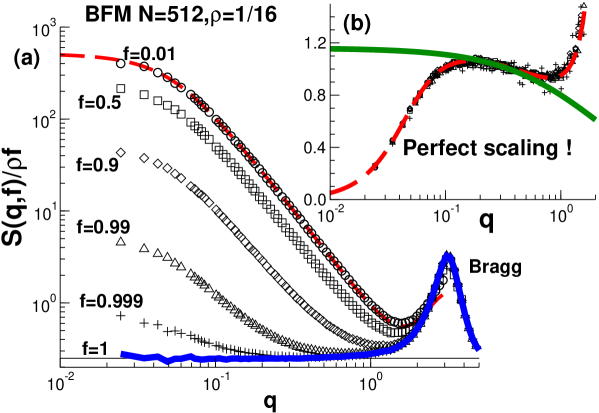
At this point one may wonder whether eq 1, (the precise form of this equation being given in the caption of Figure 10) routinely used to rationalize the scattering of a mixture of deuterated and hydrogenated chains is accurate enough to extract the form factor, including the corrections. From a theoretical point of view, for “ideal” labeling of the chains, which does not introduce additional interactions between labeled and unlabeled chains, there is no question that this can be done. Practically however, there is a danger that experimental noise in subtracted terms in eq 1 will mask corrections discussed in our paper. The strongest support comes here from numerical results presented in Figure 10. We have computed the response function $S(q,f)$ for a melt of monodisperse chains for chain length $N=512$ and different fractions $f$ of labeled chains. The main panel (a) gives $S(q,f)/f\rho$ and the form factor $F(q)$ as a function of the wavevector. The inset (b) presents a Kratky representation of the rescaled structure factor: For a surprisingly large range of $f$ the data scales if the standard experimental procedure is followed and the scattering of the background density fluctuations $f^{2}S(q,f=1)$ has been properly substracted Rubinstein ; SchaferBook . The rescaled response function is identical to $F(q)$ and shows precisely the non-monotonic behavior, eq 21, and the asymptotic infinite chain limit, eq 22 (bold line in inset), predicted by our theory. This confirms that eq 1 allows indeed to extract the correct form factor and should encourage experimentalists to revisit this old, but rather pivotal question of polymer science footSQ .

For Table of Contents Use Only

Intramolecular Form Factor in Dense Polymer Systems: Systematic Deviations from the Debye formula

P. Beckrich, A. Johner, A. N. Semenov, S. P. Obukhov, H. Benoît and J. P. Wittmer

References

- (1) Flory, P.J., Statistical Mechanics of Chain Molecules (Oxford University Press, New York, 1988).
- (2) De Gennes, P.-G., Scaling Concepts in Polymer Physics (Cornell University, Ithaca, N.Y., 1979).
- (3) Doi, M.; Edwards, S.F., The Theory of Polymer Dynamics (Clarendon Press, Oxford, 1986).
- (4) Grosberg, A.Y.; Khokhlov, A.R., Statistical Physics of Macromolecules (AIP Press, New York, 1994).
- (5) Rubinstein, M.; Colby, R.H., Polymer Physics (Oxford University Press, Oxford, 2003).
- (6) Higgins, J.S.; Benoît, H.C., Polymers and Neutron Scattering (Oxford University Press, 1996).
- (7) Rawiso, M., Journal de Physique IV 1999, 9, 147.
- (8) Boué, F.; Nierlich, M.; Leibler, L., Polymer 1982, 23, 29.
- (9) Unwanted inhomogeneities (dusts or bubbles) scatter at low-, also polydispersity effects are most important there.
- (10) Rawiso, M.; Duplessix, R.; Picot, C., Macromolecules 1987, 20, 630.
- (11) Obviously, these operational problems may be overcome in the future by using very long and flexible polymers provided labelled and unlabelled chains do not demix, with the Flory parameter. For a blend of hydogenated and fully deuterated polystyrene at , Bates .
- (12) Bates, F.S.; Wignall, G.D., Physical Review Letter 1986, 57, 1429.
- (13) Semenov, A.N.; Johner, A., Eur. Phys. J. E 2003 12, 469.
- (14) Wittmer, J.P.; Meyer, H.; Baschnagel, J.; Johner, A.; Obukhov, S.P.; Mattioni, L.; Müller, M.; Semenov, A.N.; Phys. Rev. Lett. 2004, 93, 147801.
- (15) Semenov, A.N.; Obukhov, S.P., J. Phys.: Condens. Matter 2005, 17, S1747.
- (16) Obukhov, S.P.; Semenov, A.N., Phys. Rev. Lett. 2005, 95, 038305.
- (17) Wittmer, J.P.; Beckrich, P.; Johner, A.; Semenov, A.N.; Obukhov, S.P.; Meyer, H.; Baschnagel, J., Europhysics Letters 2007, accepted.
- (18) Beckrich, P.; Correlation properties of linear polymers in the bulk and near interfaces, PhD thesis, Université Louis Pasteur, Strasbourg, France 2006.
- (19) Cavallo, A.; Müller, M.; Wittmer, J.P.; Johner, A., J. Phys.: Condens. Matter 2005, 17, 1697.
- (20) Curro, J.G.; Schweizer, K.S.; Grest, G.S; Kremer, K., J. Chem. Phys. 1991, 91, 1359.
- (21) Auhl, R.; Everaers, R.; Grest, G.S.; Kremer, K.; Plimpton, S.J, J. Chem. Phys. 2003, 119, 12718.
- (22) Sommer, J.-U.; Saalwachter, K., EPJ E 2005, 18, 167.
- (23) Svaneborg, C.; Grest, G.S.; Everaers, R., Europhys. Lett. 2005, 72, 760.
- (24) A more subtle effect arises from the mean-field treatment (implicitly allowing for cycles ANSSO2005 ; SOANSPRL2005 ) of the bath surrounding the chain under consideration. This can be shown to be negligible.
- (25) Carmesin, I.; Kremer, K., Macromolecules 1988, 21, 2819; Paul, W.; Binder, K.; Heermann, D.; Kremer, K., J. Phys. II 1991, 1, 37.
- (26) Baschnagel, J.; Wittmer, J.P.; Meyer, H., Monte Carlo Simulation of Polymers: Coarse-Grained Models, in Computational Soft Matter: From Synthetic Polymers to Proteins edited by N. Attig et al. (NIC Series, Volume 23, Jülich, 2004), pp. 83-140.
- (27) Cates, M.E.; Candau, S.J.; J. Phys. Cond. Matt 1990, 2, 6869.
- (28) Wittmer, J.P.; Milchev, A.; Cates, M.E., J.Chem. Phys. 1998, 109, 834.
- (29) Huang, C.C.; Xu, H.; Crevel, F.; Wittmer, J.P.; Ryckaert, J.-P., Lect. Notes Phys. (Springer) 2006, 704, 379; cond-mat/0604279.
- (30) Note that there is no difference between the annealed and the corresponding quenched polydispersity for infinite macroscopically homogeneous systems as long as equilibrium properties (static rather than dynamic properties) are concerned. This follows from the well-known behavior of fluctuations of extensive parameters (like mean molecular weight, or polydispersity degree) in macroscopic systems: the relative fluctuations vanish as as the total volume .
- (31) Edwards, S.F., Proc. Phys. Soc. 1965, 85, 613.
- (32) Edwards, S.F., Proc. Phys. Soc. 1966, 88, 265.
- (33) Des Cloizeaux, J.; Jannink, G., Polymers in Solution : their Modelling and Structure (Clarendon Press, Oxford, 1990).
- (34) Pines, D.; Nozieres, P., The Theory of Quantum Liquids Vol.I (W.A. Benjamin, Inc, New York, 1966).
- (35) Ohta, T.; Nakanishi, A., J. Phys. A: Math. Gen. 1983, 16, 4155.
- (36) Duplantier, B., J. Stat. Phys. 1986, 47, 1633.
- (37) Edwards, S.F., J.Phys.A: Math.Gen. 1975, 8, 1670.
- (38) Muthukumar, M.; Edwards, S.E., J. Chem. Phys. 1982, 76, 2720.
- (39) Nikomarov, E.S.; Obukhov, S.P., Sov. Phys. — JETP 1981, 53, 328.
- (40) The full cumbersome expression leading to eq 12 is not given here.
- (41) Khoklov, A.R.; Semenov, A.N., Journal of Statistical Physics 1985, 38, 161.
- (42) Abramowitz, M.; Stegun, I.A., Handbook of Mathematical Functions (Dover, New York, 1964).
- (43) Schäfer, L., Excluded Volume Effects in Polymer Solutions (Springer-Verlag, New York, 1999).
- (44) Schäfer, L.; Müller, M.; Binder, K., Macromolecules 2000, 33, 4568.
- (45) Obukhov, S.P., Phys. Rev. Lett. 1990, 65, 1395.
- (46) Berge, P.; Pomeau, Y.; Vidal, C., Order within Chaos (Hermann, Paris, 1988).
- (47) This result has been cross-checked by means of a direct perturbation calculation for monodisperse chains using the Padé approximation of Debye’s formula for the effective interaction potential.
-
(48)
As indicated in jojoPRL may be best obtained from the
intramolecular (mean-squared) distance averaged
over all monomer pairs of the chains. As suggested by eq 17
one plots as a function of
which allows the simple one-parameter fit:
The prefactor — derived in Ref. jojoPRL , eq 2., for monodisperse chains — does also apply to polydisperse systems provided . Note that it is in principle also possible to obtain from the total coil size as indicated by eqs 15 and 16 for the polydisperse case. Due to chain end effects it turns out that this requires much larger (mean) chain lengths than the recommended method above. - (49) Wittmer, J.P., et al., in preparation.
- (50) Since the EP chains break and recombine permanently the relaxation time of the system is not set by the typical EP radius of gyration but rather by the size of a small chain segment which has just about the time to diffuse over its radius before it breaks or recombines CC90 . The high frequency for the scission-recombination attempts used in our simulations ensures that the effective recombination time is small and the dynamics is, hence, always of Rouse-type. It should be emphasized that due to the permanent recombination events a data structure based on a topologically ordered intra chain interactions is not appropriate and straight-forward pointer lists between connected monomers are required WMC98 . The attempt frequency should not by taken too large to avoid useless immediate recombination of the same monomers and some time must be given for the monomers to diffuse over a couple of monomer diameters between scission-recombination attempts HXCWR06 .
- (51) Fuchs, M., Z. Phys. B 1997, 521-530.
- (52) Schulz, M.; Frisch, H.L.; Reineker, P., New Journal of Physics 2004, 6, 77.
- (53) We have computed the response function for monodisperse polymers over a large range of densities and for a nouvel version of the BFM with finite overlap energies. This has been done to verify the recent prediction of fluctuation induced long-range repulsions between solid objects in polymer media ANSSO2005 ; SOANSPRL2005 . This approach suggests a systematic violation of the RPA eq 2 proportional to which we have put to a numerical test. Our findings — complicated by the fact that trivial monomer-monomer correlations of Percus-Yevick type Fuchs ; Schulz must be correctly taken into account footMFcycles — will be presented elsewhere. Please note that these corrections to eq 2 do correspond to higher order deviations which can be shown to be negligible for the questions addressed in this paper.