Introduction to the theory of stochastic processes and Brownian motion problems

These notes are an introduction to the theory of stochastic processes based on several sources. The presentation mainly follows the books of van Kampen [5] and Wio [6], except for the introduction, which is taken from the book of Gardiner [2] and the parts devoted to the Langevin equation and the methods for solving Langevin and Fokker–Planck equations, which are based on the book of Risken [4].

1 Historical introduction

Theoretical science up to the end of the nineteenth century can be roughly viewed as the study of solutions of differential equations and the modelling of natural phenomena by deterministic solutions of these differential equations. It was at that time commonly thought that if all initial (and contour) data could only be collected, one would be able to predict the future with certainty.

We now know that this is not so, in at least two ways. First, the advent of quantum mechanics gave rise to a new physics, which had as an essential ingredient a purely statistical element (the measurement process). Secondly, the concept of chaos has arisen, in which even quite simple differential equations have the rather alarming property of giving rise to essentially unpredictable behaviours.

Chaos and quantum mechanics are not the subject of these notes, but we shall deal with systems were limited predictability arises in the form of fluctuations due to the finite number of their discrete constituents, or interaction with its environment (the “thermal bath”), etc. Following Gardiner [2] we shall give a semi-historical outline of how a phenomenological theory of fluctuating phenomena arose and what its essential points are.

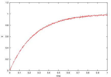
Figure 1: Schematic time evolution of a variable $X$ with a well defined deterministic motion plus fluctuations around it.

The experience of careful measurements in science normally gives us data like that of Fig. 1, representing the time evolution of a certain variable $X$. Here a quite well defined deterministic trend is evident, which is reproducible, unlike the fluctuations around this motion, which are not. This evolution could represent, for instance, the growth of the (normalised) number of molecules of a substance $X$ formed by a chemical reaction of the form $A\rightleftharpoons X$, or the process of charge of a capacitor in a electrical circuit, etc.

1.1 Brownian motion

The observation that, when suspended in water, small pollen grains are found to be in a very animated and irregular state of motion, was first systematically investigated by Robert Brown in 1827, and the observed phenomenon took the name of Brownian motion. This motion is illustrated in Fig. 2. Being a botanist, he of course tested whether this motion was in some way a manifestation of life. By showing that the motion was present in any suspension of fine particles —glass, mineral, etc.— he ruled out any specifically organic origin of this motion.

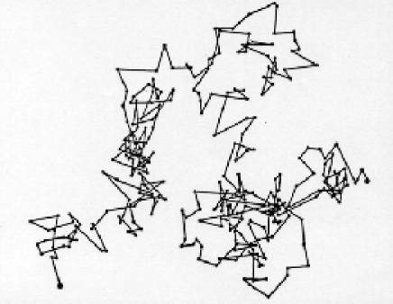
Figure 2: Motion of a particle undergoing Brownian motion.

1.1.1 Einstein’s explanation (1905)

A satisfactory explanation of Brownian motion did not come until 1905, when Einstein published an article entitled Concerning the motion, as required by the molecular-kinetic theory of heat, of particles suspended in liquids at rest. The same explanation was independently developed by Smoluchowski in 1906, who was responsible for much of the later systematic development of the theory. To simplify the presentation, we restrict the derivation to a one-dimensional system.

There were two major points in Einstein’s solution of the problem of Brownian motion:

• The motion is caused by the exceedingly frequent impacts on the pollen grain of the incessantly moving molecules of liquid in which it is suspended.

• The motion of these molecules is so complicated that its effect on the pollen grain can only be described probabilistically in term of exceedingly frequent statistically independent impacts.

Einstein development of these ideas contains all the basic concepts which make up the subject matter of these notes. His reasoning proceeds as follows: “It must clearly be assumed that each individual particle executes a motion which is independent of the motions of all other particles: it will also be considered that the movements of one and the same particle in different time intervals are independent processes, as long as these time intervals are not chosen too small.”

“We introduce a time interval $\tau$ into consideration, which is very small compared to the observable time intervals, but nevertheless so large that in two successive time intervals $\tau$, the motions executed by the particle can be thought of as events which are independent of each other.”

“Now let there be a total of $n$ particles suspended in a liquid. In a time interval $\tau$, the $X$-coordinates of the individual particles will increase by an amount $\Delta$, where for each particle $\Delta$ has a different (positive or negative) value. There will be a certain frequency law for $\Delta$; the number ${\rm d}n$ of the particles which experience a shift between $\Delta$ and $\Delta+{\rm d}\Delta$ will be expressible by an equation of the form: ${\rm d}n=n\,\phi(\Delta){\rm d}\Delta$, where $\int_{-\infty}^{\infty}\phi(\Delta){\rm d}\Delta=1$, and $\phi$ is only different from zero for very small values of $\Delta$, and satisfies the condition $\phi(-\Delta)=\phi(\Delta)$.”

“We now investigate how the diffusion coefficient depends on $\phi$. We shall restrict ourselves to the case where the number of particles per unit volume depends only on $x$ and $t$.”

“Let $f(x,t)$ be the number of particles per unit volume. We compute the distribution of particles at the time $t+\tau$ from the distribution at time $t$. From the definition of the function $\phi(\Delta)$, it is easy to find the number of particles which at time $t+\tau$ are found between two planes perpendicular to the $x$-axis and passing through points $x$ and $x+{\rm d}x$. One obtains:

$${\framebox{$\displaystyle{f(x,t+\tau){\rm d}x={\rm d}x\int_{-\infty}^{\infty}f(x+\Delta,t)\phi(\Delta){\rm d}\Delta\;.}$}}$$ (1.1)

But since $\tau$ is very small, we can set

$$f(x,t+\tau)=f(x,t)+\tau\frac{\partial f}{\partial t}\;.$$

Furthermore, we expand $f(x+\Delta,t)$ in powers of $\Delta$:

$$f(x+\Delta,t)=f(x,t)+\Delta\frac{\partial f(x,t)}{\partial x}+\frac{\Delta^{2}}{2!}\frac{\partial^{2}f(x,t)}{\partial x^{2}}+\cdots\;.$$

We can use this series under the integral, because only small values of $\Delta$ contribute to this equation. We obtain

$${\framebox{$\displaystyle{f+\tau\frac{\partial f}{\partial t}=f\int_{-\infty}^{\infty}\phi(\Delta){\rm d}\Delta+\frac{\partial f}{\partial x}\int_{-\infty}^{\infty}\Delta\,\phi(\Delta){\rm d}\Delta+\frac{\partial^{2}f}{\partial x^{2}}\int_{-\infty}^{\infty}\frac{\Delta^{2}}{2}\phi(\Delta){\rm d}\Delta\;.}$}}$$ (1.2)

Because $\phi(-\Delta)=\phi(\Delta)$, the second, fourth, etc. terms on the right-hand side vanish, while out of the 1st, 3rd, 5th, etc., terms, each one is very small compared with the previous. We obtain from this equation, by taking into consideration

$$\int_{-\infty}^{\infty}\phi(\Delta){\rm d}\Delta=1\;.$$

and setting

$$\frac{1}{\tau}\int_{-\infty}^{\infty}\frac{\Delta^{2}}{2}\phi(\Delta){\rm d}\Delta=D\;,$$ (1.3)

and keeping only the 1st and 3rd terms of the right hand side,

$${\framebox{$\displaystyle{\frac{\partial f}{\partial t}=D\frac{\partial^{2}f}{\partial x^{2}}\;.}$}}$$ (1.4)

This is already known as the differential equation of diffusion and it can be seen that $D$ is the diffusion coefficient.”

“The problem, which correspond to the problem of diffusion from a single point (neglecting the interaction between the diffusing particles), is now completely determined mathematically: its solution is

$$f(x,t)=\frac{1}{\sqrt{\pi\,4Dt}}\,e^{-x^{2}/4Dt}\;.$$ (1.5)

This is the solution, with the initial condition of all the Brownian particles initially at $x=0$; this distribution is shown in Fig. 3

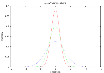
Figure 3: Time evolution of the non-equilibrium probability distribution (1.5).

Einstein ends with: “We now calculate, with the help of this equation, the displacement $\lambda_{x}$ in the direction of the $X$-axis that a particle experiences on the average or, more exactly, the square root of the arithmetic mean of the square of the displacements in the direction of the $X$-axis; it is

$$\lambda_{x}=\sqrt{\left\langle x^{2}\right\rangle-\left\langle x_{0}^{2}\right\rangle}=\sqrt{2\,D\,t}\;.$$ (1.6)

Einstein derivation contains very many of the major concepts which since then have been developed more and more generally and rigorously over the years, and which will be the subject matter of these notes. For example:

1. The Chapman–Kolgomorov equation occurs as Eq. (1.1). It states that the probability of the particle being at point $x$ at time $t+\tau$ is given by the sum of the probabilities of all possible “pushes” $\Delta$ from positions $x+\Delta$, multiplied by the probability of being at $x+\Delta$ at time $t$. This assumption is based on the independence of the push $\Delta$ of any previous history of the motion; it is only necessary to know the initial position of the particle at time $t$—not at any previous time. This is the Markov postulate and the Chapman–Kolmogorov equation, of which Eq. (1.1) is a special form, is the central dynamical equation to all Markov processes. These will be studied in Sec. 3.

2. The Kramers–Moyal expansion. This is the expansion used [Eq. (1.2)] to go from Eq. (1.1) (the Chapman–Kolmogorov equation) to the diffusion equation (1.4).

3. The Fokker–Planck equation. The mentioned diffusion equation (1.4), is a special case of a Fokker–Planck equation. This equation governs an important class of Markov processes, in which the system has a continuous sample path. We shall consider points (ii) and (iii) in detail in Sec. 4.

1.1.2 Langevin’s approach (1908)

Some time after Einstein’s work, Langevin presented a new method which was quite different from the former and, according to him, “infiniment plus simple”. His reasoning was as follows.

From statistical mechanics, it was known that the mean kinetic energy of the Brownian particles should, in equilibrium, reach the value

$$\left\langle\tfrac{1}{2}mv^{2}\right\rangle=\tfrac{1}{2}k_{{\rm B}}T\;.$$ (1.7)

Acting on the particle, of mass $m$, there should be two forces:

1. a viscous force: assuming that this is given by the same formula as in macroscopic hydrodynamics, this is $-m\gamma{\rm d}x/{\rm d}t$, with $m\gamma=6\pi\mu a$, being $\mu$ the viscosity and $a$ the diameter of the particle.

2. a fluctuating force $\xi(t)$, which represents the incessant impacts of the molecules of the liquid on the Brownian particle. All what we know about it is that is indifferently positive and negative and that its magnitude is such that maintains the agitation of the particle, which the viscous resistance would stop without it.

Thus, the equation of motion for the position of the particle is given by Newton’s law as

$${\framebox{$\displaystyle{m\frac{{\rm d}^{2}x}{{\rm d}t^{2}}=-m\gamma\,\frac{{\rm d}x}{{\rm d}t}+\xi(t)\;.}$}}$$ (1.8)

Multiplying by $x$, this can be written

$$\frac{m}{2}\frac{{\rm d}^{2}(x^{2})}{{\rm d}t^{2}}-mv^{2}=-\frac{m\gamma}{2}\frac{{\rm d}(x^{2})}{{\rm d}t}+\xi\,x\;.$$

If we consider a large number of identical particles, average this equation written for each one of them, and use the equipartition result (1.7) for $\left\langle mv^{2}\right\rangle$, we get and equation for $\left\langle x^{2}\right\rangle$

$$\frac{m}{2}\frac{{\rm d}^{2}\left\langle x^{2}\right\rangle}{{\rm d}t^{2}}+\frac{m\gamma}{2}\frac{{\rm d}\left\langle x^{2}\right\rangle}{{\rm d}t}=k_{{\rm B}}T\;.$$

The term $\left\langle\xi\,x\right\rangle$ has been set to zero because (to quote Langevin) “of the irregularity of the quantity $\xi(t)$”. One then finds the solution ($C$ is an integration constant)

$$\frac{{\rm d}\left\langle x^{2}\right\rangle}{{\rm d}t}=2k_{{\rm B}}T/m\gamma+Ce^{-\gamma t}\;.$$

Langevin estimated that the decaying exponential approaches zero with a time constant of the order of $10^{-8}$ s, so that ${\rm d}\left\langle x^{2}\right\rangle/{\rm d}t$ enters rapidly a constant regime ${\rm d}\left\langle x^{2}\right\rangle/{\rm d}t=2k_{{\rm B}}T/m\gamma$ Therefore, one further integration (in this asymptotic regime) leads to

$$\left\langle x^{2}\right\rangle-\left\langle x_{0}^{2}\right\rangle=2(k_{{\rm B}}T/m\gamma)t\;,$$

which corresponds to Einstein result (1.6), provided we identify the diffusion coefficient as

$${\framebox{$\displaystyle{D=k_{{\rm B}}T/m\gamma\;.}$}}$$ (1.9)

It can be seen that Einstein’s condition of the independence of the displacements $\Delta$ at different times, is equivalent to Langevin’s assumption about the vanishing of $\left\langle\xi\,x\right\rangle$. Langevin’s derivation is more general, since it also yields the short time dynamics (by a trivial integration of the neglected $Ce^{-\gamma t}$), while it is not clear where in Einstein’s approach this term is lost.

Langevin’s equation was the first example of a stochastic differential equation— a differential equation with a random term $\xi(t)$ and hence whose solution is, in some sense, a random function. Each solution of the Langevin equation represents a different random trajectory and, using only rather simple properties of the fluctuating force $\xi(t)$, measurable results can be derived. Figure 4 shows the trajectory of a Brownian particle in two dimensions obtained by numerical integration of the Langevin equation (we shall also study numerical integration of stochastic differential equations).

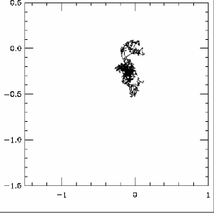
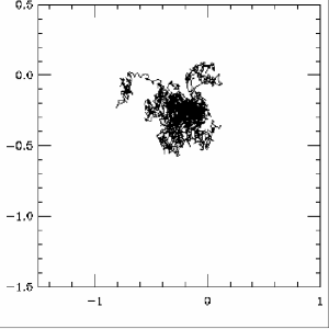
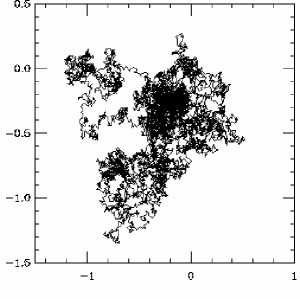
Figure 4: Trajectory of a simulated Brownian particle projected into the $x$-$y$ plane, with $D=0.16$ $\mu$ m²/s. The $x$ and $y$ axes are marked in microns. It starts from the origin $(x,y)=(0,0)$ at $t=0$, and the pictures show the trajectory after 1 sec, 3 sec and 10 sec.

It is seen the growth with $t$ of the area covered by the particle, which corresponds to the increase of $\left\langle x^{2}\right\rangle-\left\langle x_{0}^{2}\right\rangle$ in the one-dimensional case discussed above.

The theory and experiments on Brownian motion during the first two decades of the XX century, constituted the most important indirect evidence of the existence of atoms and molecules (which were unobservable at that time). This was a strong support for the atomic and molecular theories of matter, which until the beginning of the century still had strong opposition by the so-called energeticits. The experimental verification of the theory of Brownian motion awarded the 1926 Nobel price to Svedberg and Perrin.

The picture of a Brownian particle immersed in a fluid is typical of a variety of problems, even when there are no real particles. For instance, it is the case if there is only a certain (slow or heavy) degree of freedom that interacts, in a more or less irregular or random way, with many other (fast or light) degrees of freedom, which play the role of the bath. Thus, the general concept of fluctuations describable by Fokker–Planck and Langevin equations has developed very extensively in a very wide range of situations. A great advantage is the necessity of only a few parameters; in the example of the Brownian particle, essentially the coefficients of the derivatives in the Kramers–Moyal expansion (allowing in general the coefficients a $x$ and $t$ dependence)

$$\int_{-\infty}^{\infty}\Delta\,\phi(\Delta){\rm d}\Delta\;,\qquad\int_{-\infty}^{\infty}\frac{\Delta^{2}}{2}\phi(\Delta){\rm d}\Delta\;,\ldots\;.$$ (1.10)

It is rare to find a problem (mechanical oscillators, fluctuations in electrical circuits, chemical reactions, dynamics of dipoles and spins, escape over metastable barriers, etc.) with cannot be specified, in at least some degree of approximation, by the corresponding Fokker–Planck equation, or equivalently, by augmenting a deterministic differential equation with some fluctuating force or field, like in Langevin’s approach. In the following sections we shall describe the methods developed for a systematic and more rigorous study of these equations.

2 Stochastic variables

2.1 Single variable case

A stochastic or random variable is a quantity $X$, defined by a set of possible values $\{x\}$ (the “range”, “sample space”, or “phase space”), and a probability distribution on this set, $P_{X}(x)$. The range can be discrete or continuous, and the probability distribution is a non-negative function, $P_{X}(x)\geq 0$, with $P_{X}(x){\rm d}x$ the probability that $X\in(x,x+{\rm d}x)$. The probability distribution is normalised in the sense

$$\int\!{\rm d}x\,P_{X}(x)=1\;,$$

where the integral extends over the whole range of $X$.

In a discrete range, $\{x_{n}\}$, the probability distribution consists of a number of delta-type contributions, $P_{X}(x)=\sum_{n}p_{n}\delta(x-x_{n})$ and the above normalisation condition reduces to $\sum_{n}p_{n}=1$. For instance, consider the usual example of casting a die: the range is $\{x_{n}\}=\{1,2,3,4,5,6\}$ and $p_{n}=1/6$ for each $x_{n}$ (in a honest die). Thus, by allowing $\delta$-function singularities in the probability distribution, one may formally treat the discrete case by the same expressions as those for the continuous case.

2.1.1 Averages and moments

The average of a function $f(X)$ defined on the range of the stochastic variable $X$, with respect to the probability distribution of this variable, is defined as

$$\left\langle{f(X)}\right\rangle=\int\!{\rm d}x\,f(x)P_{X}(x)\;.$$

The moments of the stochastic variable, $\mu_{m}$, correspond to the special cases $f(X)=X^{m}$, i.e.,

$$\mu_{m}=\left\langle{X^{m}}\right\rangle=\int\!{\rm d}x\,x^{m}P_{X}(x)\;,\qquad m=1,2,\ldots\;.$$ (2.1)

2.1.2 Characteristic function

This useful quantity is defined by the average of $\exp(\mathrm{i}kX)$, namely

$$G_{X}(k)=\left\langle{\exp(\mathrm{i}kX)}\right\rangle=\int\!{\rm d}x\,\exp(\mathrm{i}kx)P_{X}(x)\;.$$ (2.2)

This is merely the Fourier transform of $P_{X}(x)$, and can naturally be solved for the probability distribution

$$P_{X}(x)=\frac{1}{2\pi}\int_{-\infty}^{\infty}{\rm d}k\,\exp(-\mathrm{i}kx)G_{X}(k)\;.$$

The function $G_{X}(k)$ provides an alternative complete characterisation of the probability distribution.

By expanding the exponential in the integrand of Eq. (2.2) and interchanging the order of the resulting series and the integral, one gets

$$G_{X}(k)=\sum_{m=0}^{\infty}\frac{(\mathrm{i}k)^{m}}{m!}\int\!{\rm d}x\,x^{m}P_{X}(x)=\sum_{m=0}^{\infty}\frac{(\mathrm{i}k)^{m}}{m!}\mu_{m}\;.$$ (2.3)

Therefore, one finds that $G_{X}(k)$ is the moment generating function, in the sense that

$$\mu_{m}=(-i)^{m}\left.{\frac{\partial{{}^{m}}}{\partial{k^{m}}}G_{X}(k)}\right|_{{k=0}}\;.$$ (2.4)

2.1.3 Cumulants

The cumulants, $\kappa_{m}$, are defined as the coefficients of the expansion of the cumulant function $\ln G_{X}(k)$ in powers of $\mathrm{i}k$, that is,

$$\ln G_{X}(k)=\sum_{m=1}^{\infty}\frac{(\mathrm{i}k)^{m}}{m!}\kappa_{m}\;.$$

Note that, owing to $P_{X}(x)$ is normalised, the $m=0$ term vanishes and the above series begins at $m=1$. The explicit relations between the first four cumulants and the corresponding moments are

$$\begin{array}[]{rcl}\kappa_{1}&=&\mu_{1}\\[4.30554pt] \kappa_{2}&=&\mu_{2}-\mu_{1}^{2}\\[4.30554pt] \kappa_{3}&=&\mu_{3}-3\mu_{2}\mu_{1}+2\mu_{1}^{3}\\[4.30554pt] \kappa_{4}&=&\mu_{4}-4\mu_{3}\mu_{1}-3\mu_{2}^{2}+12\mu_{2}\mu_{1}^{2}-6\mu_{1}^{4}\;.\end{array}$$ (2.5)

Thus, the first cumulant is coincident with the first moment (mean) of the stochastic variable: $\kappa_{1}=\left\langle{X}\right\rangle$; the second cumulant $\kappa_{2}$, also called the variance and written $\sigma^{2}$, is related to the first and second moments via $\sigma^{2}\equiv\kappa_{2}=\left\langle{X^{2}}\right\rangle-\left\langle{X}\right\rangle^{2}$. We finally mention that there exists a general expression for $\kappa_{m}$ in terms of the determinant of a $m\times m$ matrix constructed with the moments $\{\mu_{i}\mid i=1,\ldots,m\}$ (see, e.g., [4, p. 18]):

$$\kappa_{m}=(-1)^{m-1}\left|\begin{array}[]{cccccc}\mu_{1}&1&0&0&0&\ldots\\[4.30554pt] \mu_{2}&\mu_{1}&1&0&0&\ldots\\[4.30554pt] \mu_{3}&\mu_{2}&{2\choose 1}\mu_{1}&1&0&\ldots\\[4.30554pt] \mu_{4}&\mu_{3}&{3\choose 1}\mu_{2}&{3\choose 2}\mu_{1}&1&\ldots\\[4.30554pt] \mu_{5}&\mu_{4}&{4\choose 1}\mu_{3}&{4\choose 2}\mu_{2}&{4\choose 3}\mu_{1}&\ldots\\[4.30554pt] \ldots&\ldots&\ldots&\ldots&\ldots&\ldots\end{array}\right|_{m}\;.$$ (2.6)

where the ${i\choose k}$ are binomial coefficients.

2.2 Multivariate probability distributions

All the above definitions, corresponding to one variable, are readily extended to higher-dimensional cases. Consider the $n$-dimensional vector of stochastic variables ${\bf{X}}=(X_{1},\ldots,X_{n})$, with a probability distribution $P_{n}(x_{1},\ldots,x_{n})$. This distribution is also referred to as the joint probability distribution and

$$P_{n}(x_{1},\ldots,x_{n}){\rm d}x_{1}\cdots{\rm d}x_{n}\;,$$

is the probability that $X_{1},\ldots,X_{n}$ have certain values between $(x_{1},x_{1}+{\rm d}x_{1})$,…, $(x_{n},x_{n}+{\rm d}x_{n})$.

Partial distributions.

One can also consider the probability distribution for some of the variables. This can be done in various ways:

1. Take a subset of $s<n$ variables $X_{1},\ldots,X_{s}$. The probability that they have certain values in $(x_{1},x_{1}+{\rm d}x_{1}),\ldots,(x_{s},x_{s}+{\rm d}x_{s})$, regardless of the values of the remaining variables $X_{s+1},\ldots,X_{n}$, is

   $$P_{s}(x_{1},\ldots,x_{s})=\int\!{\rm d}x_{s+1}\cdots{\rm d}x_{n}\,P_{n}(x_{1},\ldots,x_{s},x_{s+1},\ldots,x_{n})\;,$$

   which is called the marginal distribution for the subset $X_{1},\ldots,X_{s}$. Note that from the normalisation of the joint probability it immediately follows the normalisation of the marginal probability.

2. Alternatively, one may attribute fixed values to $X_{s+1},\ldots,X_{n}$, and consider the joint probability of the remaining variables $X_{1},\ldots,X_{s}$. This is called the conditional probability, and it is denoted by

   $$P_{s|n-s}(x_{1},\ldots,x_{s}|x_{s+1},\ldots,x_{n})\;.$$

   This distribution is constructed in such a way that the total joint probability $P_{n}(x_{1},\ldots,x_{n})$ is equal to the marginal probability for $X_{s+1},\ldots,X_{n}$ to have the values $x_{s+1},\ldots,x_{n}$, times the conditional probability that, this being so, the remaining variables $X_{1},\ldots,X_{s}$ have the values $(x_{1},\ldots,x_{s})$. This is Bayes’ rule, and can be considered as the definition of the conditional probability:

   $$P_{n}(x_{1},\ldots,x_{n})=P_{n-s}(x_{s+1},\ldots,x_{n})P_{s|n-s}(x_{1},\ldots,x_{s}|x_{s+1},\ldots,x_{n})\;.$$

   Note that from the normalisation of the joint and marginal probabilities it follows the normalisation of the conditional probability.

Characteristic function: moments and cumulants.

For multivariate probability distributions, the moments are defined by

$$\left\langle{X_{1}^{m_{1}}\cdots X_{n}^{m_{n}}}\right\rangle=\int\!{\rm d}x_{1}\cdots{\rm d}x_{n}\,x_{1}^{m_{1}}\cdots x_{n}^{m_{n}}P(x_{1},\ldots,x_{n})\;,$$

while the characteristic (moment generating) function depends on $n$ auxiliary variables ${\bf{k}}=(k_{1},\ldots,k_{n})$:

$$G({\bf{k}}) = \left\langle{\exp[\mathrm{i}(k_{1}X_{1}+\cdots+k_{n}X_{n})]}\right\rangle$$ (2.7)

$$= \sum_{0}^{\infty}\frac{(\mathrm{i}k_{1})^{m_{1}}\cdots(\mathrm{i}k_{n})^{m_{n}}}{m_{1}!\cdots m_{n}!}\left\langle{X_{1}^{m_{1}}\cdots X_{n}^{m_{n}}}\right\rangle\;.$$

Similarly, the cumulants of the multivariate distribution, indicated by double brackets, are defined in terms of the coefficients of the expansion of $\ln G$ as

$$\ln G({\bf{k}})=\sum_{0}^{\infty}{}^{\prime}\frac{(\mathrm{i}k_{1})^{m_{1}}\cdots(\mathrm{i}k_{n})^{m_{n}}}{m_{1}!\cdots m_{n}!}\left\langle{\left\langle{X_{1}^{m_{1}}\cdots X_{n}^{m_{n}}}\right\rangle}\right\rangle\;,$$

where the prime indicates the absence of the term with all the $m_{i}$ simultaneously vanishing (by the normalisation of $P_{n}$).

Covariance matrix.

The second-order moments may be combined into a $n$ by $n$ matrix $\left\langle{X_{i}X_{j}}\right\rangle$. More relevant is, however, the covariance matrix, defined by the second-order cumulants

$$\left\langle{\left\langle{X_{i}X_{j}}\right\rangle}\right\rangle=\left\langle{X_{i}X_{j}}\right\rangle-\left\langle{X_{i}}\right\rangle\left\langle{X_{j}}\right\rangle=\left\langle{[X_{i}-\left\langle{X_{i}}\right\rangle][X_{j}-\left\langle{X_{j}}\right\rangle]}\right\rangle\;.$$

Each diagonal element is called the variance of the corresponding variable, while the off-diagonal elements are referred to as the covariance of the corresponding pair of variables.

Statistical independence.

A relevant concept for multivariate distributions is that of statistical independence. One says that, e.g., two stochastic variables $X_{1}$ and $X_{2}$ are statistically independent of each other if their joint probability distribution factorises:

$$P_{X_{1}X_{2}}(x_{1},x_{2})=P_{X_{1}}(x_{1})P_{X_{2}}(x_{2})\;.$$

The statistical independence of $X_{1}$ and $X_{2}$ is also expressed by any one of the following three equivalent criteria:

1. All moments factorise: $\left\langle{X_{1}^{m_{1}}X_{2}^{m_{2}}}\right\rangle=\left\langle{X_{1}^{m_{1}}}\right\rangle\left\langle{X_{2}^{m_{2}}}\right\rangle\;.$

2. The characteristic function factorises: $G_{X_{1}X_{2}}(k_{1},k_{2})=G_{X_{1}}(k_{1})G_{X_{2}}(k_{2})\;.$

3. The cumulants $\left\langle{\left\langle{X_{1}^{m_{1}}X_{2}^{m_{2}}}\right\rangle}\right\rangle$ vanish when both $m_{1}$ and $m_{2}$ are $\neq 0$.

Finally, two variables are called uncorrelated when its covariance, $\left\langle{\left\langle{X_{1}X_{2}}\right\rangle}\right\rangle$, is zero, which is a condition weaker than that of statistical independence.

2.3 The Gaussian distribution

This important distribution is defined as

$$P(x)=\frac{1}{\sqrt{2\pi\sigma^{2}}}\exp\left[{-\frac{(x-\mu_{1})^{2}}{2\sigma^{2}}}\right]\;.$$ (2.8)

It is easily seen that $\mu_{1}$ is indeed the average and $\sigma^{2}$ the variance, which justifies the notation. The corresponding characteristic function is

$$G(k)=\exp(\mathrm{i}\mu_{1}k-\tfrac{1}{2}\sigma^{2}k^{2})\;,$$ (2.9)

as can be seen from the definition (2.2), by completing the square in the argument of the total exponential $\mathrm{i}kx-(x-\mu_{1})^{2}/2\sigma^{2}$ and using the Gaussian integral $\int\!{\rm d}k\,e^{-\alpha(k-b)^{2}}=\sqrt{\pi/\alpha}$ for complex $b$ as in the footnote in p. 3. Note that the logarithm of this characteristic function comprises terms up to quadratic in $k$ only. Therefore, all the cumulants after the second one vanish identically, which is a property that indeed characterises the Gaussian distribution.

For completeness, we finally write the Gaussian distribution for $n$ variables ${\bf{X}}=(X_{1},\ldots,X_{n})$ and the corresponding characteristic function

$$P({\bf{x}}) = \sqrt{\frac{\det\hat{A}}{(2\pi)^{n}}}\exp\left[{-\tfrac{1}{2}({\bf{x}}-{\bf{x}}_{0})\cdot\hat{A}\cdot({\bf{x}}-{\bf{x}}_{0})}\right]$$

$$G({\bf{k}}) = \exp\left({i{\bf{x}}_{0}\cdot{\bf{k}}-\tfrac{1}{2}{\bf{k}}\cdot\hat{A}^{-1}\cdot{\bf{k}}}\right)\;.$$

The averages and covariances are given by $\left\langle{{\bf{X}}}\right\rangle={\bf{x}}_{0}$ and $\left\langle{\left\langle{X_{i}X_{j}}\right\rangle}\right\rangle=(\hat{A}^{-1})_{ij}$.

2.4 Transformation of variables

For a given stochastic variable $X$, every related quantity $Y=f(X)$ is again a stochastic variable. The probability that $Y$ has a value between $y$ and $y+\Delta y$ is

$$P_{Y}(y)\Delta y=\int\limits_{y<f(x)<y+\Delta y}{\rm d}x\,P_{X}(x)\;,$$

where the integral extends over all intervals of the range of $X$ where the inequality is obeyed. Note that one can equivalently define $P_{Y}(y)$ as

$${\framebox{$\displaystyle{P_{Y}(y)=\int\!{\rm d}x\,\delta[y-f(x)]P_{X}(x)\;.}$}}$$ (2.11)

From this expression one can calculate the characteristic function of $Y$:

$$G_{Y}(k) \stackrel{{\scriptstyle\text{Eq.\ (\ref{charfunc})}}}{{=}} \int\!{\rm d}y\,\exp(\mathrm{i}ky)P_{Y}(y)$$

$$= \int\!{\rm d}x\,P_{X}(x)\int\!{\rm d}y\,\exp(\mathrm{i}ky)\delta[y-f(x)]$$

$$= \int\!{\rm d}x\,P_{X}(x)\exp[\mathrm{i}kf(x)]\;,$$

which can finally be written as

$${\framebox{$\displaystyle{G_{Y}(k)=\left\langle{\exp[\mathrm{i}kf(X)]}\right\rangle\;.}$}}$$ (2.12)

As the simplest example consider the linear transformation $Y=\alpha X$. The above equation then yields $G_{Y}(k)=\left\langle{\exp(\mathrm{i}k\alpha X)}\right\rangle$, whence

$$G_{Y}(k)=G_{X}(\alpha k)\;,\qquad(Y=\alpha X)\;.$$ (2.13)

2.5 Addition of stochastic variables

The above equations for the transformation of variables remain valid when $X$ stands for a stochastic variable with $n$ components and $Y$ for one with $s$ components, where $s$ may or may not be equal to $n$. For example, let us consider the case of the addition of two stochastic variables $Y=f(X_{1},X_{2})=X_{1}+X_{2}$, where $s=1$ and $n=2$. Then, from Eq. (2.11) one first gets

$$P_{Y}(y) = \int\!{\rm d}x_{1}\,\int\!{\rm d}x_{2}\,\delta[y-(x_{1}+x_{2})]P_{X_{1}X_{2}}(x_{1},x_{2})$$ (2.14)

$$= \int\!{\rm d}x_{1}\,P_{X_{1}X_{2}}(x_{1},y-x_{1})\;.$$

Properties of the sum of stochastic variables.

One easily deduces the following three rules concerning the addition of stochastic variables:

1. Regardless of whether $X_{1}$ and $X_{2}$ are independent or not, one has

   $$\left\langle{Y}\right\rangle=\left\langle{X_{1}}\right\rangle+\left\langle{X_{2}}\right\rangle\;.$$ (2.15)

2. If $X_{1}$ and $X_{2}$ are uncorrelated, $\left\langle{\left\langle{X_{1}X_{2}}\right\rangle}\right\rangle=0$, a similar relation holds for the variances

   $$\left\langle{\left\langle{Y^{2}}\right\rangle}\right\rangle=\left\langle{\left\langle{X_{1}^{2}}\right\rangle}\right\rangle+\left\langle{\left\langle{X_{2}^{2}}\right\rangle}\right\rangle\;.$$ (2.16)

3. The characteristic function of $Y=X_{1}+X_{2}$ is

   $$G_{Y}(k)=G_{X_{1}X_{2}}(k,k)\;.$$ (2.17)

On the other hand, if $X_{1}$ and $X_{2}$ are independent, Eq. (2.14) and the factorization of $P_{X_{1}X_{2}}$ and $G_{X_{1}X_{2}}$ yields

$$P_{Y}(y)=\int\!{\rm d}x_{1}\,P_{X_{1}}(x_{1})P_{X_{2}}(y-x_{1})\;,\qquad G_{Y}(k)=G_{X_{1}}(k)G_{X_{2}}(k)\;.$$ (2.18)

Thus, the probability distribution of the sum of two independent variables is the convolution of their individual probability distributions. Correspondingly, the characteristic function of the sum [which is the Fourier transform of the probability distribution; see Eq. (2.2)] is the product of the individual characteristic functions.

2.6 Central limit theorem

As a particular case of transformation of variables, one can also consider the sum of an arbitrary number of stochastic variables. Let $X_{1},\ldots,X_{n}$ be a set of $n$ independent stochastic variables, each having the same probability distribution $P_{X}(x)$ with zero average and (finite) variance $\sigma^{2}$. Then, from Eqs. (2.15) and (2.16) it follows that their sum $Y=X_{1}+\cdots+X_{n}$ has zero average and variance $n\sigma^{2}$, which grows linearly with $n$. On the other hand, the distribution of the arithmetic mean of the variables, $(X_{1}+\cdots+X_{n})/n$, becomes narrower with increasing $n$ (variance $\sigma^{2}/n$). It is therefore more convenient to define a suitable scaled sum

$$Z=\frac{X_{1}+\cdots+X_{n}}{\sqrt{n}}\;,$$

which has variance $\sigma^{2}$ for all $n$.

The central limit theorem states that, even when $P_{X}(x)$ is not Gaussian, the probability distribution of the $Z$ so-defined tends, as $n\to\infty$, to a Gaussian distribution with zero mean and variance $\sigma^{2}$. This remarkable result is responsible for the important rôle of the Gaussian distribution in all fields in which statistics are used and, in particular, in the equilibrium and non-equilibrium statistical physics.

Proof of the central limit theorem.

We begin by expanding the characteristic function of an arbitrary $P_{X}(x)$ with zero mean as [cf. Eq. (2.3)]

$$G_{X}(k)=\int\!{\rm d}x\,\exp(\mathrm{i}kx)P_{X}(x)=1-\tfrac{1}{2}\sigma^{2}k^{2}+\cdots\;.$$ (2.19)

The factorization of the characteristic function of the sum $Y=X_{1}+\cdots+X_{n}$ of statistically independent variables [Eq. (2.18)], yields

$$G_{Y}(k)=\prod_{i=1}^{n}G_{X_{i}}(k)=\left[{G_{X}(k)}\right]^{n}\;,$$

where the last equality follows from the equivalent statistical properties of the different variables $X_{i}$. Next, on accounting for $Z=Y/\sqrt{n}$, and using the result (2.13) with $\alpha=1/\sqrt{n}$, one has

$$G_{Z}(k)=G_{Y}\left({\frac{k}{\sqrt{n}}}\right)=\left[{G_{X}\left({\frac{k}{\sqrt{n}}}\right)}\right]^{n}\simeq\left({1-\frac{\sigma^{2}k^{2}}{2n}}\right)^{n}\stackrel{{\scriptstyle n\to\infty}}{{\longrightarrow}}\exp\left({-\tfrac{1}{2}\sigma^{2}k^{2}}\right)\;,\quad$$ (2.20)

where we have used the definition of the exponential $e^{x}={\displaystyle\lim_{n\to\infty}}\left({1+x/n}\right)^{n}$. Finally, on comparing the above result with Eqs. (2.8), one gets

$$P_{Z}(z)=\frac{1}{\sqrt{2\pi\sigma^{2}}}\exp\left({-\frac{z^{2}}{2\sigma^{2}}}\right)\;.\quad{\rm Q.E.D.}\quad{}$$

Remarks on the validity of the central limit theorem.

The derivation of the central limit theorem can be done under more general conditions. For instance, it is not necessary that all the cumulants (moments) exist. However, it is necessary that the moments up to at least second order exist [or, equivalently, $G_{X}(k)$ being twice differentiable at $k=0$; see Eq. (2.4)]. The necessity of this condition is illustrated by the counter-example provided by the Lorentz–Cauchy distribution:

$$P(x)=\frac{1}{\pi}\frac{\gamma}{x^{2}+\gamma^{2}}\;,\qquad(-\infty<x<\infty)\;.$$

It can be shown that, if a set of $n$ independent variables $X_{i}$ have Lorentz–Cauchy distributions, their sum also has a Lorentz–Cauchy distribution (see footnote below). However, for this distribution the conditions for the central limit theorem to hold are not met, since the integral (2.1) defining the moments $\mu_{m}$, does not converge even for $m=1$.

Finally, although the condition of independence of the variables is important, it can be relaxed to incorporate a sufficiently weak statistical dependence.

2.7 Exercise: marginal and conditional probabilities and moments of a bivariate Gaussian distribution

To illustrate the definitions given for multivariate distributions, let us compute them for a simple two-variable Gaussian distribution

$$P_{2}(x_{1},x_{2})=\sqrt{\frac{1-\lambda^{2}}{(2\pi\sigma^{2})^{2}}}\exp\left[-\frac{1}{2\sigma^{2}}\left(x_{1}^{2}-2\lambda\,x_{1}x_{2}+x_{2}^{2}\right)\right]\;,$$ (2.23)

where $\lambda$ is a parameter $-1<\lambda<1$, to ensure that the quadratic form in the exponent is definite positive (the equivalent condition to assume $\sigma^{2}$ to be positive in the one-variable Gaussian distribution (2.8). The normalisation factor can be seen to take this value by direct integration, or by comparing our distribution with the multidimensional Gaussian distribution (Sec. 2.3); here $\hat{A}=\displaystyle\frac{1}{\sigma^{2}}\left(\begin{array}[]{cc}1&-\lambda\\[-2.15277pt] -\lambda&1\end{array}\right)$ so that $\det\hat{A}=(1-\lambda^{2})/\sigma^{4}$. Finally, if one wishes to fix ideas one can interpret $P_{2}(x_{1},x_{2})$ as the Boltzmann distribution of two harmonic oscillators coupled by a potential term $\propto\lambda\,x_{1}x_{2}$.

Let us first rewrite the distribution in a form that will facilitate to do the integrals by completing once more the square $-2\lambda\,x_{1}x_{2}+x_{2}^{2}=(x_{2}-\lambda x_{1})^{2}-\lambda^{2}x_{1}^{2}$

$$P_{2}(x_{1},x_{2})=C\exp\left[-\frac{1-\lambda^{2}}{2\sigma^{2}}x_{1}^{2}\right]\,\exp\left[-\frac{1}{2\sigma^{2}}(x_{2}-\lambda x_{1})^{2}\right]\;.$$ (2.24)

and $C=\sqrt{(1-\lambda^{2})/(2\pi\sigma^{2})^{2}}$ is the normalisation constant. We can now compute the marginal probability of the individual variables (for one of them since they are equivalent), defined by $P_{1}(x_{1})=\int{\rm d}x_{2}\,P_{2}(x_{1},x_{2})$

$$P_{1}(x_{1})=C\,e^{-\frac{1-\lambda^{2}}{2\sigma^{2}}x_{1}^{2}}\underbrace{\int\!{\rm d}x_{2}\,e^{-(x_{2}-\lambda x_{1})^{2}/2\sigma^{2}}}_{\sqrt{\pi/\alpha}\quad\alpha=1/2\sigma^{2}}\;.$$

Therefore, recalling the form of $C$, we merely have

$$P_{1}(x_{1})=\frac{1}{\sqrt{2\pi\sigma_{\lambda}^{2}}}\,\exp\left(-\frac{x_{1}^{2}}{2\sigma_{\lambda}^{2}}\right)\;,\qquad\mbox{with}\qquad\sigma_{\lambda}^{2}=\sigma^{2}/(1-\lambda^{2})\;.$$ (2.25)

We see that the marginal distribution depends on $\lambda$, which results in a modified variance. To see that $\sigma_{\lambda}^{2}$ is indeed the variance $\left\langle{\left\langle{x_{1}^{2}}\right\rangle}\right\rangle=\left\langle{x_{1}^{2}}\right\rangle-\left\langle{x_{1}}\right\rangle^{2}$, note that $\left\langle x_{1}^{m}\right\rangle$ can be obtained from the marginal distribution only (this is a general result)

$$\left\langle x_{1}^{m}\right\rangle=\int\!{\rm d}x_{1}\int\!{\rm d}x_{2}\,x_{1}^{m}P_{2}(x_{1},x_{2})=\int\!{\rm d}x_{1}\,x_{1}^{m}\!\underbrace{\int\!{\rm d}x_{2}\,P_{2}(x_{1},x_{2})}_{P_{1}(x_{1})}=\int\!{\rm d}x_{1}\,x_{1}^{m}P_{1}(x_{1})$$

Then inspecting the marginal distribution obtained [Eq. (2.25)] we get that the first moments vanish and the variances are indeed equal to $\sigma_{\lambda}^{2}$:

$${\framebox{$\displaystyle{\begin{array}[]{rclcrcl}\left\langle x_{1}\right\rangle&=&0&&\left\langle x_{2}\right\rangle&=&0\\[4.30554pt] \left\langle x_{1}^{2}\right\rangle&=&\sigma_{\lambda}^{2}&&\left\langle x_{2}^{2}\right\rangle&=&\sigma_{\lambda}^{2}\end{array}}$}}$$ (2.26)

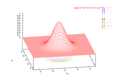
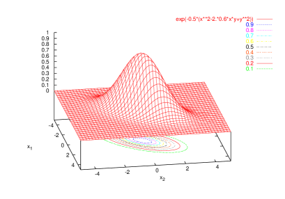
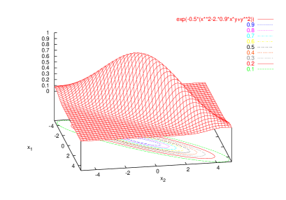
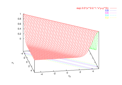
Figure 5: Gaussian distribution (2.23) for $\lambda=0$, $0.6$, $0.9$ and $1$ (non-normalised).

To complete the calculation of the moments up to second order we need the covariance of $x_{1}$ and $x_{2}$: $\left\langle{\left\langle{x_{1}x_{2}}\right\rangle}\right\rangle=\left\langle{x_{1}x_{2}}\right\rangle-\left\langle{x_{1}}\right\rangle\left\langle{x_{2}}\right\rangle$ which reduces to calculate $\left\langle x_{1}x_{2}\right\rangle$. This can be obtained using the form (2.24) for the distribution

$$\left\langle x_{1}x_{2}\right\rangle = \int\!{\rm d}x_{1}\int\!{\rm d}x_{2}\,x_{1}x_{2}P_{2}(x_{1},x_{2})$$

$$= C\int\!{\rm d}x_{1}x_{1}\exp\left[-\frac{1-\lambda^{2}}{2\sigma^{2}}x_{1}^{2}\right]\overbrace{\int\!{\rm d}x_{2}\,x_{2}\exp\left[-\frac{1}{2\sigma^{2}}(x_{2}-\lambda x_{1})^{2}\right]}^{\lambda x_{1}\sqrt{2\pi\sigma^{2}}}$$

$$= \lambda\sqrt{2\pi\sigma^{2}}C\underbrace{\int\!{\rm d}x_{1}x_{1}^{2}\exp\left[-\frac{1-\lambda^{2}}{2\sigma^{2}}x_{1}^{2}\right]}_{\sqrt{2\pi\sigma^{2}/(1-\lambda^{2})}\,\sigma^{2}/(1-\lambda^{2})}\quad\Rightarrow\quad{\framebox{$\displaystyle{\left\langle x_{1}x_{2}\right\rangle=\frac{\lambda}{1-\lambda^{2}}\sigma^{2}}$}}$$

since $C=\sqrt{(1-\lambda^{2})/(2\pi\sigma^{2})^{2}}$. Its is convenient to compute the normalised covariance $\left\langle x_{1}x_{2}\right\rangle/\sqrt{\left\langle x_{1}^{2}\right\rangle\left\langle x_{2}^{2}\right\rangle}$, which is merely given by $\lambda$. Therefore the parameter $\lambda$ in the distribution (2.23) is a measure of how much correlated the variables $x_{1}$ and $x_{2}$ are. Actually in the limit $\lambda\to 0$ the variables are not correlated at all and the distribution factorises. In the opposite limit $\lambda\to 1$ the variables are maximally correlated, $\left\langle x_{1}x_{2}\right\rangle/\sqrt{\left\langle x_{1}^{2}\right\rangle\left\langle x_{2}^{2}\right\rangle}=1$. The distribution is actually a function of $(x_{1}-x_{2})$, so it is favoured that $x_{1}$ and $x_{2}$ take similar values (see Fig. 5)

$$P_{2}|_{\lambda=0}=\frac{1}{\sqrt{2\pi\sigma^{2}}}\,e^{-x_{1}^{2}/2\sigma^{2}}\frac{1}{\sqrt{2\pi\sigma^{2}}}\,e^{-x_{2}^{2}/2\sigma^{2}},\quad P_{2}|_{\lambda=1}\to e^{-(x_{1}-x_{2})^{2}/2\sigma^{2}}\;.$$ (2.27)

We can now interpret the increase of the variances with $\lambda$: the correlation between the variables allows them to take arbitrarily large values, with the only restriction of their difference being small (Fig. 5).

To conclude we can compute the conditional probability by using Bayes rule $P_{1|1}(x_{1}|x_{2})=P_{2}(x_{1},x_{2})/P_{1}(x_{2})$ and Eqs. (2.23) and (2.25)

$$P_{1|1}(x_{1}|x_{2}) = \frac{\sqrt{\frac{1-\lambda^{2}}{(2\pi\sigma^{2})^{2}}}\exp\left[-\frac{1}{2\sigma^{2}}\left(x_{1}^{2}-2\lambda\,x_{1}x_{2}+x_{2}^{2}\right)\right]}{\sqrt{\frac{1-\lambda^{2}}{2\pi\sigma^{2}}}\,\exp\left(-\frac{1-\lambda^{2}}{2\sigma^{2}}x_{2}^{2}\right)}$$

$$= \frac{1}{\sqrt{2\pi\sigma^{2}}}\exp\left[-\frac{1}{2\sigma^{2}}\left(x_{1}^{2}-2\lambda\,x_{1}x_{2}+[{{}\not}1-({{}\not}1-\lambda^{2})]x_{2}^{2}\right)\right]\;,$$

and hence (recall that here $x_{2}$ is a parameter; the known output of $X_{2}$)

$$P_{1|1}(x_{1}|x_{2})=\frac{1}{\sqrt{2\pi\sigma^{2}}}\exp\left[-\frac{1}{2\sigma^{2}}\left(x_{1}-\lambda\,x_{2}\right)^{2}\right]\;.$$ (2.28)

Then, at $\lambda=0$ (no correlation) the values taken by $x_{1}$ are independent of the output of $x_{2}$ while for $\lambda\to 1$ they are centered around those taken by $x_{2}$, and hence strongly conditioned by them.

3 Stochastic processes and Markov processes

Once a stochastic variable $X$ has been defined, an infinity of other stochastic variables derive from it, namely, all the quantities $Y$ defined as functions of $X$ by some mapping. These quantities $Y$ may be any kind of mathematical object; in particular, also functions of an auxiliary variable $t$:

$$Y_{X}(t)=f(X,t)\;,$$

where $t$ could be the time or some other parameter. Such a quantity $Y_{X}(t)$ is called a stochastic process. On inserting for $X$ one of its possible values $x$, one gets an ordinary function of $t$, $Y_{x}(t)=f(x,t)$, called a sample function or realisation of the process. In physical language, one regards the stochastic process as the “ensemble” of these sample functions.

It is easy to form averages on the basis of the underlying probability distribution $P_{X}(x)$. For instance, one can take $n$ values $t_{1},\ldots,t_{n}$, and form the $n$th moment

$$\left\langle{Y(t_{1})\cdots Y(t_{n})}\right\rangle=\int\!{\rm d}x\,Y_{x}(t_{1})\cdots Y_{x}(t_{n})P_{X}(x)\;.$$ (3.1)

Of special interest is the auto-correlation function

$$\kappa(t_{1},t_{2})\equiv\left\langle{\left\langle{Y(t_{1})Y(t_{2})}\right\rangle}\right\rangle = \left\langle{Y(t_{1})Y(t_{2})}\right\rangle-\left\langle{Y(t_{1})}\right\rangle\left\langle{Y(t_{2})}\right\rangle$$

$$= \big{\langle}{[Y(t_{1})-\left\langle{Y(t_{1})}\right\rangle][Y(t_{2})-\left\langle{Y(t_{2})}\right\rangle]}\big{\rangle}\;,$$

which, for $t_{1}=t_{2}=t$, reduces to the time-dependent variance $\left\langle{\left\langle{Y(t)^{2}}\right\rangle}\right\rangle=\sigma(t)^{2}$.

A stochastic process is called stationary when the moments are not affected by a shift in time, that is, when

$$\left\langle{Y(t_{1}+\tau)\cdots Y(t_{n}+\tau)}\right\rangle=\left\langle{Y(t_{1})\cdots Y(t_{n})}\right\rangle\;.$$ (3.2)

In particular, $\left\langle{Y(t)}\right\rangle$ is then independent of the time, and the auto-correlation function $\kappa(t_{1},t_{2})$ only depends on the time difference $|t_{1}-t_{2}|$. Often there exist a constant $\tau_{c}$ such that $\kappa(t_{1},t_{2})\simeq 0$ for $|t_{1}-t_{2}|>\tau_{c}$; one then calls $\tau_{c}$ the auto-correlation time of the stationary stochastic process.

If the stochastic quantity consist of several components $Y_{i}(t)$, the auto-correlation function is replaced by the correlation matrix

$$K_{ij}(t_{1},t_{2})=\left\langle{\left\langle{Y_{i}(t_{1})Y_{j}(t_{2})}\right\rangle}\right\rangle\;.$$

The diagonal elements are the auto-correlations and the off-diagonal elements are the cross-correlations. Finally, in case of a zero-average stationary stochastic process, this equation reduces to

$$K_{ij}(\tau)=\left\langle{Y_{i}(t)Y_{j}(t+\tau)}\right\rangle=\left\langle{Y_{i}(0)Y_{j}(\tau)}\right\rangle\;.$$

3.1 The hierarchy of distribution functions

A stochastic process $Y_{X}(t)$, defined from a stochastic variable $X$ in the way described above, leads to a hierarchy of probability distributions. For instance, the probability distribution for $Y_{X}(t)$ to take the value $y$ at time $t$ is [cf. Eq. (2.11)]

$$P_{1}(y,t)=\int\!{\rm d}x\,\delta[y-\underbrace{Y_{x}(t)}_{f(x,t)}]P_{X}(x)\;.$$

Similarly, the joint probability distribution that $Y$ has the value $y_{1}$ at $t_{1}$, and also the value $y_{2}$ at $t_{2}$, and so on up to $y_{n}$ at $t_{n}$, is

$$P_{n}(y_{1},t_{1};\ldots;y_{n},t_{n})=\int\!{\rm d}x\,\delta[y_{1}-Y_{x}(t_{1})]\cdots\delta[y_{n}-Y_{x}(t_{n})]P_{X}(x)\;.$$ (3.3)

In this way an infinite hierarchy of probability distributions $P_{n}$, $n=1,2,\ldots$, is defined. They allow one the computation of all the averages already introduced, e.g.,

$$\left\langle{Y(t_{1})\cdots Y(t_{n})}\right\rangle=\int\!{\rm d}y_{1}\cdots{\rm d}y_{n}\,y_{1}\cdots y_{n}P_{n}(y_{1},t_{1};\ldots;y_{n},t_{n})\;.$$ (3.4)

We note in passing that, by means of this result, the definition (3.2) of stationary processes, can be restated in terms of the dependence of the $P_{n}$ on the time differences alone, namely

$$P_{n}(y_{1},t_{1}+\tau;\ldots;y_{n},t_{n}+\tau)=P_{n}(y_{1},t_{1};\ldots;y_{n},t_{n})\;.$$

Consequently, a necessary (but not sufficient) condition for the stochastic process being stationary is that $P_{1}(y_{1})$ does not depend on the time.

Although the right-hand side of Eq. (3.3) also has a meaning when some of the times are equal, one regards the $P_{n}$ to be defined only when all times are different. The hierarchy of probability distributions $P_{n}$ then obeys the following consistency conditions:

1. $P_{n}\geq 0\;;$

2. $P_{n}$ is invariant under permutations of two pairs $(y_{i},t_{i})$ and $(y_{j},t_{j})\;;$

3. ${\displaystyle\int}\!{\rm d}{y_{n}}\,P_{n}(y_{1},t_{1};\ldots;y_{n},t_{n})=P_{n-1}(y_{1},t_{1};\ldots;y_{n-1},t_{n-1})\;;$

4. ${\displaystyle\int}\!{\rm d}{y_{1}}\,P_{1}(y_{1},t_{1})=1\;.$

Inasmuch as the distributions $P_{n}$ enable one to compute all the averages of the stochastic process [Eq. (3.4)], they constitute a complete specification of it. Conversely, according to a theorem due to Kolmogorov, it is possible to prove that the inverse is also true, i.e., that any set of functions obeying the above four consistency conditions determines a stochastic process $Y(t)$.

3.2 Gaussian processes

A stochastic process is called a Gaussian process, if all its $P_{n}$ are multivariate Gaussian distributions (Sec. 2.3). In that case, all cumulants beyond $m=2$ vanish and, recalling that $\left\langle{\left\langle{Y(t_{1})Y(t_{2})}\right\rangle}\right\rangle=\left\langle{Y(t_{1})Y(t_{2})}\right\rangle-\left\langle{Y(t_{1})}\right\rangle\left\langle{Y(t_{2})}\right\rangle$, one sees that a Gaussian process is fully specified by its average $\left\langle{Y(t)}\right\rangle$ and its second moment $\left\langle{Y(t_{1})Y(t_{2})}\right\rangle$. Gaussian stochastic processes are often used as an approximate description for physical processes, which amounts to assuming that the higher-order cumulants are negligible.

3.3 Conditional probabilities

The notion of conditional probability for multivariate distributions can be applied to stochastic processes, via the hierarchy of probability distributions introduced above. For instance, the conditional probability $P_{1|1}(y_{2},t_{2}|y_{1},t_{1})$ represents the probability that $Y$ takes the value $y_{2}$ at $t_{2}$, given that its value at $t_{1}$ “was” $y_{1}$. It can be constructed as follows: from all sample functions $Y_{x}(t)$ of the ensemble representing the stochastic process, select those passing through the point $y_{1}$ at the time $t_{1}$; the fraction of this sub-ensemble that goes through the gate $(y_{2},y_{2}+{\rm d}y_{2})$ at the time $t_{2}$ is precisely $P_{1|1}(y_{2},t_{2}|y_{1},t_{1}){\rm d}y_{2}$. More generally, one may fix the values of $Y$ at $n$ different times $t_{1},\ldots,t_{n}$, and ask for the joint probability at $m$ other times $t_{n+1},\ldots,t_{n+m}$. This leads to the general definition of the conditional probability $P_{m|n}$ by Bayes’ rule:

$$P_{m|n}(y_{n+1},t_{n+1};\ldots;y_{n+m},t_{n+m}|y_{1},t_{1};\ldots;y_{n},t_{n})=\frac{P_{n+m}(y_{1},t_{1};\ldots;y_{n+m},t_{n+m})}{P_{n}(y_{1},t_{1};\ldots;y_{n},t_{n})}\;.$$ (3.5)

Note that the right-hand side of this equation is well defined in terms of the probability distributions of the hierarchy $P_{n}$ previously introduced. Besides, from their consistency conditions it follows the normalisation of the $P_{m|n}$.

3.4 Markov processes

Among the many possible classes of stochastic processes, there is one that merits a special treatment—the so-called Markov processes.

Recall that, for a stochastic process $Y(t)$, the conditional probability $P_{1|1}(y_{2},t_{2}|y_{1},t_{1})$, is the probability that $Y(t_{2})$ takes the value $y_{2}$, provided $Y(t_{1})$ has taken the value $y_{1}$. In terms of this quantity one can express $P_{2}$ as

$$P_{2}(y_{1},t_{1};y_{2},t_{2})=P_{1}(y_{1},t_{1})P_{1|1}(y_{2},t_{2}|y_{1},t_{1})\;.$$ (3.6)

However, to construct the higher-order $P_{n}$ one needs transition probabilities $P_{n|m}$ of higher order, e.g., $P_{3}(y_{1},t_{1};y_{2},t_{2};y_{3},t_{3})=P_{2}(y_{1},t_{1};y_{2},t_{2})P_{1|2}(y_{3},t_{3}|y_{1},t_{1};y_{2},t_{2})$. A stochastic process is called a Markov process, if for any set of $n$ successive times $t_{1}<t_{2}<\cdots<t_{n}$, one has

$$P_{1|n-1}(y_{n},t_{n}|y_{1},t_{1};\ldots;y_{n-1},t_{n-1})=P_{1|1}(y_{n},t_{n}|y_{n-1},t_{n-1})\;.$$ (3.7)

In words: the conditional probability distribution of $y_{n}$ at $t_{n}$, given the value $y_{n-1}$ at $t_{n-1}$, is uniquely determined, and is not affected by any knowledge of the values at earlier times.

A Markov process is therefore fully determined by the two distributions $P_{1}(y,t)$ and $P_{1|1}(y^{\prime},t^{\prime}|y,t)$, from which the entire hierarchy $P_{n}(y_{1},t_{1};\ldots;y_{n},t_{n})$ can be constructed. For instance, consider $t_{1}<t_{2}<t_{3}$; $P_{3}$ can be written as

$$P_{3}(y_{1},t_{1};y_{2},t_{2};y_{3},t_{3}) \stackrel{{\scriptstyle\text{Eq.\ (\ref{bayesrule:2})}}}{{=}}P_{2}(y_{1},t_{1};y_{2},t_{2})P_{1|2}(y_{3},t_{3}|y_{1},t_{1};y_{2},t_{2})$$ (3.8)

$$\stackrel{{\scriptstyle\text{Eq.\ (\ref{markov})}}}{{=}}P_{2}(y_{1},t_{1};y_{2},t_{2})P_{1|1}(y_{3},t_{3}|y_{2},t_{2})$$

$$\stackrel{{\scriptstyle\text{Eq.\ (\ref{bayesrule:particular})}}}{{=}}P_{1}(y_{1},t_{1})P_{1|1}(y_{2},t_{2}|y_{1},t_{1})P_{1|1}(y_{3},t_{3}|y_{2},t_{2})\;.\quad$$

From now on, we shall only deal with Markov processes. Then, the only independent conditional probability is $P_{1|1}(y^{\prime},t^{\prime}|y,t)$, so we shall omit the subscript $1|1$ henceforth and call $P_{1|1}(y^{\prime},t^{\prime}|y,t)$ the transition probability.

3.5 Chapman–Kolmogorov equation

Let us now derive an important identity that must be obeyed by the transition probability of any Markov process. On integrating Eq. (3.8) over $y_{2}$, one obtains ($t_{1}<t_{2}<t_{3}$)

$$P_{2}(y_{1},t_{1};y_{3},t_{3})=P_{1}(y_{1},t_{1}){\displaystyle\int}\!{\rm d}{y_{2}}\,P(y_{2},t_{2}|y_{1},t_{1})P(y_{3},t_{3}|y_{2},t_{2})\;,$$

where the consistency condition 3 of the hierarchy of distribution functions $P_{n}$ has been used to write the left-hand side. Now, on dividing both sides by $P_{1}(y_{1},t_{1})$ and using the special case (3.6) of Bayes’ rule, one gets

$${\framebox{$\displaystyle{P(y_{3},t_{3}|y_{1},t_{1})={\displaystyle\int}\!{\rm d}{y_{2}}\,P(y_{3},t_{3}|y_{2},t_{2})P(y_{2},t_{2}|y_{1},t_{1})\;,}$}}$$ (3.9)

which is called the Chapman–Kolmogorov equation. The time ordering is essential: $t_{2}$ must lie between $t_{1}$ and $t_{3}$ for Eq. (3.9) to hold. This is required in order to the starting Eq. (3.8) being valid, specifically, in order to the second equality there being derivable from the first one by dint of the definition (3.7) of a Markov process.

Note finally that, on using Eq. (3.6) one can rewrite the particular case $P_{1}(y_{2},t_{2})=\int{\rm d}y_{1}\,P_{2}(y_{2},t_{2};y_{1},t_{1})$ of the relation among the distributions of the hierarchy as

$${\framebox{$\displaystyle{P_{1}(y_{2},t_{2})={\displaystyle\int}\!{\rm d}{y_{1}}\,P(y_{2},t_{2}|y_{1},t_{1})P_{1}(y_{1},t_{1})\;.}$}}$$ (3.10)

This is an additional relation involving the two probability distributions characterising a Markov process. Reciprocally, any non-negative functions obeying Eqs. (3.9) and (3.10), define a Markov process uniquely.

3.6 Examples of Markov processes

Wiener–Lévy process.

This stochastic process was originally introduced in order to describe the behaviour of the position of a free Brownian particle in one dimension. On the other hand, it plays a central rôle in the rigorous foundation of the stochastic differential equations. The Wiener–Lévy process is defined in the range $-\infty<y<\infty$ and $t>0$ through [cf. Eq. (1.5)]

$$\halign to=0.0pt{\@eqnsel\hskip\@centering$\displaystyle{#}$&\global\@eqcnt\@ne\hskip 2\arraycolsep\hfil${#}$\hfil&\global\@eqcnt\tw@\hskip 2\arraycolsep$\displaystyle{#}$\hfil&\llap{#}\cr 0.0pt plus 1000.0pt$\displaystyle{ {} P_{1}(y_{1},t_{1}) &10.0pt\hfil${=&10.0pt$\displaystyle{\frac{1}{\sqrt{2\pi t_{1}}} \exp\left({-\frac{y_{1}^{2}}{2t_{1}}}\right) \;, {}&\hbox to0.0pt{\hss{\rm(3.11a)}\cr\penalty 100\vskip 3.0pt\vskip 0.0pt\cr 0.0pt plus 1000.0pt$\displaystyle{{} P(y_{2},t_{2}|y_{1},t_{1}) &10.0pt\hfil${=&10.0pt$\displaystyle{\frac{1}{\sqrt{2\pi(t_{2}-t_{1})}} \exp\left[{-\frac{(y_{2}-y_{1})^{2}}{2(t_{2}-t_{1})}}\right] \;, \quad(t_{1}<t_{2}) \;. \qquad&\hbox to0.0pt{\hss{\rm(3.11b)}\cr}}}}}}}}}$$

This is a non-stationary ($P_{1}$ depends on $t$), Gaussian process. The second-order moment is

$$\left\langle{Y(t_{1})Y(t_{2})}\right\rangle = \min(t_{1},t_{2})\;,$$ (3.12)

Proof: Let us assume $t_{1}<t_{2}$. Then, from Eq. (3.4) we have

$$\left\langle{Y(t_{1})Y(t_{2})}\right\rangle = {\displaystyle\int}\!{\rm d}{y_{1}}\,{\displaystyle\int}\!{\rm d}{y_{2}}\,y_{1}y_{2}P_{2}(y_{1},t_{1};y_{2},t_{2})$$

$$= {\displaystyle\int}\!{\rm d}{y_{1}}\,y_{1}P_{1}(y_{1},t_{1})\underbrace{{\displaystyle\int}\!{\rm d}{y_{2}}\,y_{2}P(y_{2},t_{2}|y_{1},t_{1})}_{y_{1}\;\text{by~{}Eq.\ (\ref{wienerlevy:Ptrans})}}=\underbrace{{\displaystyle\int}\!{\rm d}{y_{1}}\,y_{1}^{2}P_{1}(y_{1},t_{1})}_{t_{1}~{}\text{by~{}Eq.\ (\ref{wienerlevy:P1})}}\;,$$

where we have used that $t_{1}$ is the time-dependent variance of $P_{1}$.  Q.E.D.

Ornstein–Uhlenbeck process.

This stochastic process was constructed to describe the behaviour of the velocity of a free Brownian particle in one dimension (see Sec. 4.5). It also describes the position of an overdamped particle in an harmonic potential. It is defined by ($\Delta t=t_{2}-t_{1}>0$)

$$\halign to=0.0pt{\@eqnsel\hskip\@centering$\displaystyle{#}$&\global\@eqcnt\@ne\hskip 2\arraycolsep\hfil${#}$\hfil&\global\@eqcnt\tw@\hskip 2\arraycolsep$\displaystyle{#}$\hfil&\llap{#}\cr 0.0pt plus 1000.0pt$\displaystyle{ {} P_{1}(y_{1}) &10.0pt\hfil${=&10.0pt$\displaystyle{\frac{1}{\sqrt{2\pi}}\exp\left({-\tfrac{1}{2}y_{1}^{2}}\right) \;, {}&\hbox to0.0pt{\hss{\rm(3.13a)}\cr\penalty 100\vskip 3.0pt\vskip 0.0pt\cr 0.0pt plus 1000.0pt$\displaystyle{{} P(y_{2},t_{2}|y_{1},t_{1}) &10.0pt\hfil${=&10.0pt$\displaystyle{\frac{1}{\sqrt{2\pi(1-e^{-2\Delta t})}} \exp\left[{-\frac{(y_{2}-y_{1}e^{-\Delta t})^{2}}{2(1-e^{-2\Delta t})}}\right] \;. &\hbox to0.0pt{\hss{\rm(3.13b)}\cr}}}}}}}}}$$

The Ornstein–Uhlenbeck process is stationary, Gaussian, and Markovian. According to a theorem due to Doob, it is essentially the only process with these three properties. Concerning the Gaussian property, it is clear for $P_{1}(y_{1})$. For $P_{2}(y_{2},t_{2};y_{1},t_{1})=P_{1}(y_{1})P(y_{2},t_{2}|y_{1},t_{1})$ [Eq. (3.6)], we have

$$P_{2}(y_{2},t_{2};y_{1},t_{1})=\frac{1}{\sqrt{(2\pi)^{2}(1-e^{-2\Delta t})}}\exp\left[{-\frac{y_{1}^{2}-2y_{1}y_{2}e^{-\Delta t}+y_{2}^{2}}{2(1-e^{-2\Delta t})}}\right]\;.$$ (3.14)

This expression can be identified with the bivariate Gaussian distribution (2.23) and the following parameters

$$\lambda=e^{-\Delta t}\;,\qquad\sigma^{2}=1-e^{-2\Delta t}\;,$$

with the particularity that $\sigma^{2}=1-\lambda^{2}$ in this case. Therefore, we immediately see that the Ornstein–Uhlenbeck process has an exponential auto-correlation function $\left\langle{Y(t_{1})Y(t_{2})}\right\rangle=e^{-\Delta t}$, since $\sigma^{2}\lambda/(1-\lambda^{2})=\lambda$ in this case.

The evolution with time of the distribution $P_{2}(y_{2},t_{2};y_{1},t_{1})$, seen as the velocity of a Brownian particle, has a clear meaning. At short times the velocity is strongly correlated with itself: then $\lambda\sim 1$ and the distribution would be like in the lower right panel of Fig. 5 [with a shrinked variance $\sigma^{2}=(1-\lambda^{2})\to 0$]. As time elapses $\lambda$ decreases and we pass form one panel to the previous and, at long times, $\lambda\sim 0$ and the velocity has lost all memory of its value at the initial time due to the collisions and hence $P_{2}(y_{2},t_{2};y_{1},t_{1})$ is completely uncorrelated.

Exercise: check by direct integration that the transition probability (LABEL:ornsteinuhlenbeck:Ptrans) obeys the Chapman–Kolgomorov equation (3.9).

4 The master equation: Kramers–Moyal 
expansion and Fokker–Planck equation

The Chapman–Kolmogorov equation (3.9) for Markov processes is not of much assistance when one searches for solutions of a given problem, because it is essentially a property of the solution. However, it can be cast into a more useful form—the master equation.

4.1 The master equation

The master equation is a differential equation for the transition probability. Accordingly, in order to derive it, one needs first to ascertain how the transition probability behaves for short time differences.

Firstly, on inspecting the Chapman–Kolmogorov equation (3.9) for equal time arguments one finds the natural result

$$P(y_{3},t_{3}|y_{1},t)={\displaystyle\int}\!{\rm d}{y_{2}}\,P(y_{3},t_{3}|y_{2},t)P(y_{2},t|y_{1},t)\quad\Rightarrow\quad P(y_{2},t|y_{1},t)=\delta(y_{2}-y_{1})\;,$$

which is the zeroth-order term in the short-time behaviour of $P(y^{\prime},t^{\prime}|y,t)$. Keeping this in mind one adopts the following expression for the short-time transition probability:

$${\framebox{$\displaystyle{P(y_{2},t+\Delta t|y_{1},t)=\delta(y_{2}-y_{1})[1-a^{(0)}(y_{1},t)\Delta t]+W_{t}(y_{2}|y_{1})\Delta t+O[(\Delta t)^{2}]\;,}$}}$$ (4.1)

where $W_{t}(y_{2}|y_{1})$ is interpreted as the transition probability per unit time from $y_{1}$ to $y_{2}$ at time $t$. Then, the coefficient $1-a^{(0)}(y_{1},t)\Delta t$ is to be interpreted as the probability that no “transition” takes place during $\Delta t$. Indeed, from the normalisation of $P(y_{2},t_{2}|y_{1},t_{1})$ one has:

$$1={\displaystyle\int}\!{\rm d}{y_{2}}\,P(y_{2},t+\Delta t|y_{1},t)\simeq 1-a^{(0)}(y_{1},t)\Delta t+{\displaystyle\int}\!{\rm d}{y_{2}}\,W_{t}(y_{2}|y_{1})\Delta t\;.$$

Therefore, to first order in $\Delta t$, one gets

$$a^{(0)}(y_{1},t)={\displaystyle\int}\!{\rm d}{y_{2}}\,W_{t}(y_{2}|y_{1})\;,$$ (4.2)

which substantiates the interpretation mentioned: $a^{(0)}(y_{1},t)\Delta t$ is the total probability of escape from $y_{1}$ in the time interval $(t,t+\Delta t)$ and, thus, $1-a^{(0)}(y_{1},t)\Delta t$ is the probability that no transition takes place during this time.

Now we can derive the differential equation for the transition probability from the Chapman–Kolmogorov equation (3.9). Insertion of the above short-time expression for the transition probability in into it yields

$$P(y_{3},t_{2}+\Delta t|y_{1},t_{1}) = {\displaystyle\int}\!{\rm d}{y_{2}}\,\overbrace{P(y_{3},t_{2}+\Delta t|y_{2},t_{2})}^{\hbox to0.0pt{$\displaystyle\qquad\qquad\quad{\scriptstyle{\delta(y_{3}-y_{2})[1-a^{(0)}(y_{2},t_{2})\Delta t]+W_{t_{2}}(y_{3}|y_{2})\Delta t}}$\hss}}P(y_{2},t_{2}|y_{1},t_{1})$$

$$\simeq [1-a^{(0)}(y_{3},t_{2})\Delta t]P(y_{3},t_{2}|y_{1},t_{1})$$

$${}+\Delta t{\displaystyle\int}\!{\rm d}{y_{2}}\,W_{t_{2}}(y_{3}|y_{2})P(y_{2},t_{2}|y_{1},t_{1})\;.$$

Next, on using Eq. (4.2) to write $a^{(0)}(y_{3},t_{2})$ in terms of $W_{t_{2}}(y_{2}|y_{3})$, one has

$$\frac{1}{\Delta t}\left[{P(y_{3},t_{2}+\Delta t|y_{1},t_{1})-P(y_{3},t_{2}|y_{1},t_{1})}\right]$$

$$\simeq{\displaystyle\int}\!{\rm d}{y_{2}}\,\left[{W_{t_{2}}(y_{3}|y_{2})P(y_{2},t_{2}|y_{1},t_{1})-W_{t_{2}}(y_{2}|y_{3})P(y_{3},t_{2}|y_{1},t_{1})}\right]\;,$$

which in the limit $\Delta t\to 0$ yields, after some changes in notation ($y_{1},t_{1}\to y_{0},t_{0}$, $y_{2},t_{2}\to y^{\prime},t$, and $y_{3}\to y$), the master equation

$${\framebox{$\displaystyle{\frac{\partial{}}{\partial{t}}P(y,t|y_{0},t_{0})={\displaystyle\int}\!{\rm d}{y^{\prime}}\,\left[{W_{t}(y|y^{\prime})P(y^{\prime},t|y_{0},t_{0})-W_{t}(y^{\prime}|y)P(y,t|y_{0},t_{0})}\right]\;,}$}}$$ (4.3)

which is an integro-differential equation.

The master equation is a differential form of the Chapman–Kolmogorov equation (and sometimes it is referred to as such). Therefore, it is an equation for the transition probability $P(y,t|y_{0},t_{0})$, but not for $P_{1}(y,t)$. However, an equation for $P_{1}(y,t)$ can be obtained by using the concept of “extraction of a sub-ensemble”. Suppose that $Y(t)$ is a stationary Markov process characterised by $P_{1}(y)$ and $P(y,t|y_{0},t_{0})$. Let us define a new, non-stationary Markov process $Y^{\ast}(t)$ for $t\geq t_{0}$ by setting

$$\halign to=0.0pt{\@eqnsel\hskip\@centering$\displaystyle{#}$&\global\@eqcnt\@ne\hskip 2\arraycolsep\hfil${#}$\hfil&\global\@eqcnt\tw@\hskip 2\arraycolsep$\displaystyle{#}$\hfil&\llap{#}\cr 0.0pt plus 1000.0pt$\displaystyle{ {} P_{1}^{\ast}(y_{1},t_{1})&10.0pt\hfil${=&10.0pt$\displaystyle{P(y_{1},t_{1}|y_{0},t_{0}) \;, {}&\hbox to0.0pt{\hss{\rm(4.4a)}\cr\penalty 100\vskip 3.0pt\vskip 0.0pt\cr 0.0pt plus 1000.0pt$\displaystyle{{} P^{\ast}(y_{2},t_{2}|y_{1},t_{1})&10.0pt\hfil${=&10.0pt$\displaystyle{P(y_{2},t_{2}|y_{1},t_{1}) \;. &\hbox to0.0pt{\hss{\rm(4.4b)}\cr}}}}}}}}}$$

This is a sub-ensemble of $Y(t)$ characterised by taking the sharp value $y_{0}$ at $t_{0}$, since $P_{1}^{\ast}(y_{1},t_{0})=\delta(y_{1}-y_{0})$. More generally, one may extract a sub-ensemble in which at a given time $t_{0}$ the values of $Y^{\ast}(t_{0})$ are distributed according to a given probability distribution $p(y_{0})$:

$$P_{1}^{\ast}(y_{1},t_{1})={\displaystyle\int}\!{\rm d}{y_{0}}\,P(y_{1},t_{1}|y_{0},t_{0})p(y_{0})\;,$$ (4.5)

and $P^{\ast}(y_{2},t_{2}|y_{1},t_{1})$ as in Eq. (LABEL:subensemble:b). Physically, the extraction of a sub-ensemble means that one “prepares” the system in a certain non-equilibrium state at $t_{0}$.

By construction, the above $P_{1}^{\ast}(y_{1},t_{1})$ obey the same differential equation as the transition probability (with respect its first pair of arguments), that is, $P_{1}^{\ast}(y_{1},t_{1})$ obeys the master equation. Consequently, we may write, suppressing unessential indices,

$$\frac{\partial{P(y,t)}}{\partial{t}}={\displaystyle\int}\!{\rm d}{y^{\prime}}\,\left[{W(y|y^{\prime})P(y^{\prime},t)-W(y^{\prime}|y)P(y,t)}\right]\;.$$ (4.6)

If the range of $Y$ is a discrete set of states labelled with $n$, the equation reduces to

$$\frac{{\rm d}p_{n}(t)}{{\rm d}t}=\sum_{n^{\prime}}\left[W_{nn^{\prime}}p_{n^{\prime}}(t)-W_{n^{\prime}n}p_{n}(t)\right]\;.$$ (4.7)

In this form the meaning becomes clear: the master equation is a balance (gain–loss) equation for the probability of each state. The first term is the “gain” due to “transitions” from other “states” $n^{\prime}$ to $n$, and the second term is the “loss” due to “transitions” into other configurations. Remember that $W_{n^{\prime}n}\geq 0$ and that the term with $n=n^{\prime}$ does not contribute.

Owing to $W(y|y^{\prime})\Delta t$ is the transition probability in a short time interval $\Delta t$, it can be computed, for the system under study, by means of any available method valid for short times, e.g., by Dirac’s time-dependent perturbation theory leading to the “golden rule”. Then, the master equation serves to determine the time evolution of the system over long time periods, at the expense of assuming the Markov property.

The master equation can readily be extended to the case of a multi-component Markov process $Y_{i}(t)$, $i=1$, $2,\ldots$, $N$, on noting that the Chapman–Kolmogorov equation (3.9) is valid as it stands by merely replacing $y$ by ${\bf{y}}=(y_{1},\cdots,y_{N})$. Then, manipulations similar as those leading to Eq. (4.6) yield the multivariate counterpart of the master equation

$${\framebox{$\displaystyle{\frac{\partial{P({\bf{y}},t)}}{\partial{t}}={\displaystyle\int}\!{\rm d}{{\bf{y}}^{\prime}}\,\left[{W({\bf{y}}|{\bf{y}}^{\prime})P({\bf{y}}^{\prime},t)-W({\bf{y}}^{\prime}|{\bf{y}})P({\bf{y}},t)}\right]\;.}$}}$$ (4.8)

Example: the decay process.

Let us consider an typical example of master equation describing a decay process, in which $p_{n}(t)$ determines the probability of having at time $t$, $n$ surviving “emitters” (radioactive nuclei, excited atoms emitting photons, etc.). The transition probability in a short interval is

$$W_{n,n^{\prime}}\Delta t=\left\{\begin{array}[]{cl}0&\mbox{for}\quad n>n^{\prime}\\ \gamma n^{\prime}\Delta t&\mbox{for}\quad n=n^{\prime}-1\\ {\cal O}(\Delta t)^{2}&\mbox{for}\quad n<n^{\prime}-1\end{array}\right.$$

That is, there are not transitions to a state with more emitters (they can only decay; reabsortion is negligible), and the decay probability of more that one decay in $\Delta t$ is of higher order in $\Delta t$. The decay parameter $\gamma$ can be computed with quantum mechanical techniques. The corresponding master equation is Eq. (4.7) with $W_{n,n^{\prime}}=\gamma n^{\prime}\delta_{n,n^{\prime}-1}$

$$\frac{{\rm d}p_{n}(t)}{{\rm d}t}=W_{n,n+1}\,p_{n+1}(t)-W_{n-1,n}\,p_{n}(t)\;.$$

and hence

$$\frac{{\rm d}p_{n}(t)}{{\rm d}t}=\gamma(n+1)\,p_{n+1}(t)-\gamma n\,p_{n}(t)\;.$$ (4.9)

Without finding the complete solution for $p_{n}(t)$, we can derive the equation for the average number of surviving emitters $\left\langle N\right\rangle(t)=\sum_{n=0}^{\infty}n\,p_{n}(t)$

$$\sum_{n=0}^{\infty}n({\rm d}p_{n}/{\rm d}t) = \gamma\overbrace{\sum_{n=0}^{\infty}n(n+1)p_{n+1}}^{k=n+1}-\gamma\overbrace{\sum_{n=0}^{\infty}n^{2}p_{n}}^{n=0\to 1}$$

$$= \gamma\sum_{k=1}^{\infty}[({{}\not}k-1)k-{{}\not}k^{2}]p_{k}=-\gamma\overbrace{\sum_{k=1}^{\infty}kp_{k}}^{\left\langle N\right\rangle}\;.$$

Therefore the differential equation for $\left\langle N\right\rangle$ and its solution are:

$$\frac{{\rm d}}{{\rm d}t}\left\langle N\right\rangle=-\gamma\left\langle N\right\rangle\;,\quad\Rightarrow\quad{\framebox{$\displaystyle{\left\langle N\right\rangle(t)=n_{0}e^{-\gamma t}\;.}$}}$$ (4.10)

4.2 The Kramers–Moyal expansion and the Fokker–Planck equation

The Kramers–Moyal expansion of the master equation casts this integro-differential equation into the form of a differential equation of infinite order. It is therefore not easier to handle but, under certain conditions, one may break off after a suitable number of terms. When this is done after the second-order terms one gets a partial differential equation of second order for $P(y,t)$ called the Fokker–Planck equation.

Let us first express the transition probability $W$ as a function of the size $r$ of the jump from one configuration $y^{\prime}$ to another one $y$, and of the starting point $y^{\prime}$:

$$W(y|y^{\prime})=W(y^{\prime};r)\;,\qquad r=y-y^{\prime}\;.$$ (4.11)

The master equation (4.6) then reads,

$$\frac{\partial{P(y,t)}}{\partial{t}}={\displaystyle\int}\!{\rm d}{r}\,W(y-r;r)P(y-r,t)-P(y,t){\displaystyle\int}\!{\rm d}{r}\,W(y;-r)\;,$$ (4.12)

where the sign change associated with the change of variables $y^{\prime}\to r=y-y^{\prime}$, is absorbed in the boundaries (integration limits), by considering a symmetrical integration interval extending from $-\infty$ to $\infty$:

$${\displaystyle\int_{-\infty}^{\infty}}\!{\rm d}{y^{\prime}}\,f(y^{\prime})=-{\displaystyle\int_{y+\infty}^{y-\infty}}\!{\rm d}{r}\,f(y-r)=-{\displaystyle\int_{\infty}^{-\infty}}\!{\rm d}{r}\,f(y-r)={\displaystyle\int_{-\infty}^{\infty}}\!{\rm d}{r}\,f(y-r)\;.$$

Moreover, since finite integration limits would incorporate an additional dependence on $y$, we shall restrict our attention to problems to which the boundary is irrelevant.

Let us now assume that the changes on $y$ occur via small jumps, i.e., that $W(y^{\prime};r)$ is a sharply peaked function of $r$ but varies slowly enough with $y^{\prime}$. A second assumption is that $P(y,t)$ itself also varies slowly with $y$. It is then possible to deal with the shift from $y$ to $y-r$ in the first integral in Eq. (4.12) by means of a Taylor expansion:

$$\frac{\partial{P(y,t)}}{\partial{t}} = {\displaystyle\int}\!{\rm d}{r}\,W(y;r)P(y,t)+\sum_{m=1}^{\infty}\frac{(-1)^{m}}{m!}{\displaystyle\int}\!{\rm d}{r}\,r^{m}\frac{\partial{{}^{m}}}{\partial{y^{m}}}[W(y;r)P(y,t)]$$

$${}-P(y,t){\displaystyle\int}\!{\rm d}{r}\,W(y;-r)$$

$$= \sum_{m=1}^{\infty}\frac{(-1)^{m}}{m!}\frac{\partial{{}^{m}}}{\partial{y^{m}}}\left\{{\left[{{\displaystyle\int}\!{\rm d}{r}\,r^{m}W(y;r)}\right]P(y,t)}\right\}\;,$$

where we have used that the first and third terms on the first right-hand side cancel each other. Note that the dependence of $W(y;r)$ on its second argument $r$ is fully kept; an expansion with respect to it, is not useful as $W$ varies rapidly with $r$. Finally, on introducing the jump moments

$$a^{(m)}(y,t)={\displaystyle\int}\!{\rm d}{r}\,r^{m}W(y;r)\;,$$ (4.13)

one gets the Kramers–Moyal expansion of the master equation:

$${\framebox{$\displaystyle{\frac{\partial{P(y,t)}}{\partial{t}}=\sum_{m=1}^{\infty}\frac{(-1)^{m}}{m!}\frac{\partial{{}^{m}}}{\partial{y^{m}}}\left[{a^{(m)}(y,t)P(y,t)}\right]\;.}$}}$$ (4.14)

Formally, Eq. (4.14) is identical with the master equation and is therefore not easier to deal with, but it suggest that one may break off after a suitable number of terms. For instance, there could be situations where, for $m>2$, $a^{(m)}(y,t)$ is identically zero or negligible. In this case one is left with

$${\framebox{$\displaystyle{\frac{\partial{P(y,t)}}{\partial{t}}=-\frac{\partial{}}{\partial{y}}\left[{a^{(1)}(y,t)P(y,t)}\right]+\frac{1}{2}\frac{\partial{{}^{2}}}{\partial{y^{2}}}\left[{a^{(2)}(y,t)P(y,t)}\right]\;,}$}}$$ (4.15)

which is the celebrated Fokker–Planck equation. The first term is called the drift or transport term and the second one the diffusion term, while $a^{(1)}(y,t)$ and $a^{(2)}(y,t)$ are the drift and diffusion “coefficients”.

It is worth recalling that, being derived from the master equation, the Kramers–Moyal expansion, and the Fokker–Planck equation as a special case of it, involve the transition probability $P(y,t|y_{0},t_{0})$ of the Markov stochastic process, not its one-time probability distribution $P_{1}(y,t)$. However, they also apply to the $P_{1}^{\ast}(y,t)$ of every subprocess that can be extracted from a Markov stochastic process by imposing an initial condition [see Eqs. (4.1) and (4.5)].

4.3 The jump moments

The transition probability per unit time $W(y^{\prime}|y)$ enters in the definition (4.13) of the jump moments. Therefore, in order to calculate $a^{(m)}(y,t)$, we must use the relation (4.1) between $W(y^{\prime}|y)$ and the transition probability for short time differences.

Firstly, from Eq. (4.11) one sees that $W(y^{\prime};r)=W(y|y^{\prime})$ with $y=y^{\prime}+r$. Accordingly, one can write

$$W(y;r)=W(y^{\prime}|y)\;,\qquad y^{\prime}=y+r\;.$$

On inserting this expression in Eq. (4.13) one can write the jump moments as

$${\framebox{$\displaystyle{a^{(m)}(y,t)={\displaystyle\int}\!{\rm d}{y^{\prime}}\,(y^{\prime}-y)^{m}W(y^{\prime}|y)\;.}$}}$$ (4.16)

In order to calculate the jumps moments we introduce the quantity

$${\cal A}^{(m)}(y;\tau,t)={\displaystyle\int}\!{\rm d}{y^{\prime}}\,(y^{\prime}-y)^{m}P(y^{\prime},t+\tau|y,t)\;,\qquad(m\geq 1)\;,$$

which is the average of $[Y(t+\tau)-Y(t)]^{m}$ with sharp initial value $Y(t)=y$ (conditional average). Then, by using the short-time transition probability (4.1), one can write

$${\cal A}^{(m)}(y;\tau,t) = {\displaystyle\int}\!{\rm d}{y^{\prime}}\,(y^{\prime}-y)^{m}\left\{{\delta(y^{\prime}-y)[1-a^{(0)}(y,t)\tau]+W(y^{\prime}|y)\tau+{\cal O}(\tau^{2})}\right\}$$

$$= \tau{\displaystyle\int}\!{\rm d}{y^{\prime}}\,(y^{\prime}-y)^{m}W(y^{\prime}|y)+{\cal O}(\tau^{2})$$

$$= a^{(m)}(y,t)\tau+{\cal O}(\tau^{2})\;,\qquad(m\geq 1)\;,$$

where the integral involving the first term in the short-time transition probability vanishes due to the presence of the Dirac delta. Therefore, one can calculate the jump moments from the derivatives of the conditional averages as follows

$$a^{(m)}(y,t)=\left.{\frac{\partial}{\partial\tau}{\cal A}^{(m)}(y;\tau,t)}\right|_{{\tau=0}}\;.$$

Finally, on writing

$${\cal A}^{(m)}(y;\Delta t,t)={\displaystyle\int}\!{\rm d}{y^{\prime}}\,(y^{\prime}-y)^{m}P(y^{\prime},t+\Delta t|y,t)=\left.{\Big{\langle}{[Y(t+\Delta t)-Y(t)]^{m}}\Big{\rangle}}\right|_{{Y(t)=y}}\;,$$

one can alternatively express the jump moments as

$${\framebox{$\displaystyle{a^{(m)}(y,t)=\lim_{\Delta t\to 0}\frac{1}{\Delta t}\left.{\Big{\langle}{[Y(t+\Delta t)-Y(t)]^{m}}\Big{\rangle}}\right|_{{Y(t)=y}}\;.}$}}$$ (4.17)

In Sec. 5 below, which is devoted to the Langevin equation, we shall calculate the corresponding jump moments in terms of the short-time conditional averages by means of this formula.

4.4 Expressions for the multivariate case

The above formulae can be extended to the case of a multi-component Markov process $Y_{i}(t)$, $i=1$, $2,\ldots$, $N$. Concerning the Kramers–Moyal expansion one only needs to use the multivariate Taylor expansion to get

$$\frac{\partial P}{\partial t}=\sum_{m=1}^{\infty}\frac{(-1)^{m}}{m!}\sum_{j_{1}\ldots j_{m}}\frac{\partial^{m}}{\partial y_{j_{1}}\cdots\partial y_{j_{m}}}\left[{a_{j_{1},\ldots,j_{m}}^{(m)}({\bf{y}},t)P}\right]\;,$$ (4.18)

while the Fokker–Planck equation is then given by

$${\framebox{$\displaystyle{\frac{\partial P}{\partial t}=-\sum_{i}\frac{\partial}{\partial y_{i}}\left[{a_{i}^{(1)}({\bf{y}},t)P}\right]+\frac{1}{2}\sum_{ij}\frac{\partial^{2}}{\partial y_{i}\partial y_{j}}\left[{a_{ij}^{(2)}({\bf{y}},t)P}\right]\;.}$}}$$ (4.19)

In these equations, the jump moments are given by the natural generalisation of Eq. (4.16), namely

$$a_{j_{1},\ldots,j_{m}}^{(m)}({\bf{y}},t)={\displaystyle\int}\!{\rm d}{{\bf{y}}^{\prime}}\,(y_{j_{1}}^{\prime}-y_{j_{1}})\cdots(y_{j_{m}}^{\prime}-y_{j_{m}})W({\bf{y}}^{\prime}|{\bf{y}})\;,$$ (4.20)

and can be calculated by means of the corresponding generalisation of Eq. (4.17):

$${\framebox{$\displaystyle{a_{j_{1},\ldots,j_{m}}^{(m)}({\bf{y}},t)=\left.{\lim_{\Delta t\to 0}\frac{1}{\Delta t}\bigg{\langle}\prod_{\mu=1}^{m}[Y_{j_{\mu}}(t+\Delta t)-Y_{j_{\mu}}(t)]\bigg{\rangle}}\right|_{{Y_{k}(t)=y_{k}}},}$}}$$ (4.21)

that is, by means of the derivative of the corresponding conditional average.

4.5 Examples of Fokker–Planck equations

Diffusion equation for the position.

In Einstein’s explanation of Brownian motion he arrived at an equation of the form [see Eq. (1.4)]

$${\framebox{$\displaystyle{\frac{\partial P}{\partial t}=D\frac{\partial^{2}P}{\partial x^{2}}\;.}$}}$$ (4.22)

Comparing with the Fokker–Planck equation (4.15), we see that in this case $a^{(1)}(x,t)\equiv 0$, since no forces act on the particle and hence the net drift is zero. Similarly $a^{(2)}(x,t)=2D$, which is independent of space and time. This is because the properties of the surrounding medium are homogeneous [otherwise $D=D(x)$]. The solution of this equation for $P(x,t=0)=\delta(x)$ was Eq. (1.5), which corresponds to the Wiener–Lévy process (3.6).

This equation is a special case of the Smoluchowski equation for a particle with large damping coefficient $\gamma$ (overdamped particle), the special case corresponding to no forces acting on the particle.

Diffusion equation in phase space $(x,v)$.

The true diffusion equation of a free Brownian particle is

$${\framebox{$\displaystyle{\frac{\partial P}{\partial t}=-v\frac{\partial P}{\partial x}+\gamma\left(\frac{\partial}{\partial v}v+\frac{k_{{\rm B}}T}{m}\frac{\partial^{2}}{\partial v^{2}}\right)P\;.}$}}$$ (4.23)

This equation is the no potential limit of the Klein–Kramers equation for a particle with an arbitrary damping coefficient $\gamma$. From this equation one can obtain the diffusion equation (4.22) using singular perturbation theory, as the leading term in a expansion in powers of $1/\gamma$. Alternatively, we shall give a proof of this in the context of the Langevin equations corresponding to these Fokker–Planck equations.

We have stated without proof that the Ornstein–Uhlenbeck process describes the time evolution of the transition probability of the velocity of a free Brownian particle. We shall demonstrate this, by solving the equation for the marginal distribution for $v$ obtained from (4.23). The marginal probability is $P_{V}(v,t)=\int\!{\rm d}x\,P(x,v,t)$. Integrating Eq. (4.23) over $x$, using $\int\!{\rm d}x\,\partial_{x}P(x,v,t)=0$, since $P(x=\pm\infty,v,t)=0$, we find

$$\frac{\partial P_{V}}{\partial t}=\gamma\left(\frac{\partial}{\partial v}v+\frac{k_{{\rm B}}T}{m}\frac{\partial^{2}}{\partial v^{2}}\right)P_{V}\;.$$ (4.24)

We will see that this equation also describes the position of an overdamped particle in an harmonic potential. Thus, let us find the solution of the generic equation

$${\framebox{$\displaystyle{\tau\partial_{t}P=\partial_{y}(yP)+D\partial_{y}^{2}P\;.}$}}$$ (4.25)

Introducing the characteristic function (2.2) (so we are solving by the Fourier transform method)

$$G(k,t)=\int\!{\rm d}y\,e^{\mathrm{i}ky}P(y,t)\;,\qquad P(y,t)=\frac{1}{2\pi}\int{\rm d}k\,e^{-\mathrm{i}ky}G(k,t)\;,$$

the second order partial differential equation (4.25) transforms into a first order one

$$\tau\partial_{t}G+k\partial_{k}G=-Dk^{2}G\;,$$ (4.26)

which can be solved by means of the method of characteristics.

In this case the subsidiary system is

$$\frac{{\rm d}t}{\tau}=\frac{{\rm d}k}{k}=-\frac{{\rm d}G}{Dk^{2}G}\;.$$

Two integrals are easily obtained considering the systems $t,k$ and $k,G$:

$$\frac{{\rm d}t}{\tau} = \frac{{\rm d}k}{k}\quad\rightarrow\quad k=a\,e^{t/\tau}\quad\rightarrow\quad u=ke^{-t/\tau}=a$$

$$-Dk{\rm d}k = {\rm d}G/G\;\;\rightarrow\;\;-\tfrac{1}{2}Dk^{2}=\ln G+{\rm c}\;\;\rightarrow\;\;v=e^{-\tfrac{1}{2}Dk^{2}}G=b$$

Then, the solution $h(u,v)=0$ can be solved for $v$ as $v=\phi(u)$ with still an arbitrary function $\phi$, leading the desired general solution of Eq. (4.26)

$$G=e^{-\tfrac{1}{2}Dk^{2}}\phi(ke^{-t/\tau})\;,$$ (4.27)

by means of the methods of characteristics.

The solution for sharp initial values $P(y,t=0)=\delta(y-y_{0})$ leads to $G(k,t=0)=\exp(\mathrm{i}ky_{0})$, from which we get the functional form of $\phi$: $\phi(k)=\exp(\mathrm{i}ky_{0}+\tfrac{1}{2}Dk^{2})$. Therefore, one finally obtains for $G(k,t)$

$$G(k,t)=\exp\left[\mathrm{i}y_{0}e^{-t/\tau}\,k-\tfrac{1}{2}D(1-e^{-2t/\tau})\,k^{2}\right]\;,$$ (4.28)

which is the characteristic function of a Gaussian distribution [see Eq. (2.9)], with $\mu_{1}=y_{0}e^{-t/\tau}$ and $\sigma^{2}=D(1-e^{-2t/\tau})$. Therefore, the probability distribution solving Eq. (4.25) is

$${\framebox{$\displaystyle{P(y,t|y_{0},0)=\frac{1}{\sqrt{2\pi D(1-e^{-2t/\tau})}}\exp\left[{-\frac{(y-y_{0}e^{-t/\tau})^{2}}{2D(1-e^{-2t/\tau})}}\right]\;.}$}}$$ (4.29)

which, as stated, is the transition probability of the Ornstein–Uhlenbeck process [Eq. (LABEL:ornsteinuhlenbeck:Ptrans)]. Q.E.D.

Note finally that the parameters for the original equation for $P_{V}$ [Eq. (4.24)], are simply $\mu_{1}=v_{0}e^{-t/\tau}$ and $\sigma^{2}=(k_{{\rm B}}T/m)(1-e^{-2t/\tau})$. Thus, at long times we have $P_{V}\propto\exp(-\tfrac{1}{2}mv^{2}/k_{{\rm B}}T)$ which is simply the statistical mechanical equilibrium Boltzmann distribution for free particles.

Diffusion equation for a dipole.

The diffusion equation for a dipole moment $p$ in an electric field $E$ is (neglecting inertial effects)

$${\framebox{$\displaystyle{\zeta\frac{\partial P}{\partial t}=\frac{1}{\sin\vartheta}\frac{\partial}{\partial\vartheta}\left[\sin\vartheta\left(k_{{\rm B}}T\frac{\partial P}{\partial\vartheta}+pE\sin\vartheta P\right)\right]\;.}$}}$$ (4.30)

This equation was introduced by Debye in the 1920’s, and constitutes the first example of rotational Brownian motion. $\zeta$ is the viscosity coefficient (the equivalent to $\gamma$ in translational problems). It is easily seen that $P_{0}\propto\exp(pE\cos\vartheta/k_{{\rm B}}T)$ is the stationary solution of Eq. (4.30), which leads to the famous result for the average dipole moment of an assembly of dipoles, $\left\langle\cos\vartheta\right\rangle=\coth\alpha-1/\alpha$ with $\alpha=pE/k_{{\rm B}}T$ and to Curie’s paramagnetic law at low fields. However, Eq. (4.30) also governs non-equilibrium situations, and in particular the time evolution between different equilibrium states.

5 The Langevin equation

5.1 Langevin equation for one variable

The Langevin equation for one variable is a “differential equation” of the form [cf. Eq. (1.8)]

$${\framebox{$\displaystyle{\frac{{\rm d}y}{{\rm d}t}=A(y,t)+B(y,t)\xi(t)\;,}$}}$$ (5.1)

where $\xi(t)$ is a given stochastic process. The choice for $\xi(t)$ that renders $y(t)$ a Markov process is that of the Langevin “process” (white noise), which is Gaussian and its statistical properties are

$$\halign to=0.0pt{\@eqnsel\hskip\@centering$\displaystyle{#}$&\global\@eqcnt\@ne\hskip 2\arraycolsep\hfil${#}$\hfil&\global\@eqcnt\tw@\hskip 2\arraycolsep$\displaystyle{#}$\hfil&\llap{#}\cr 0.0pt plus 1000.0pt$\displaystyle{ {} \left\langle{\xi(t)}\right\rangle &10.0pt\hfil${=&10.0pt$\displaystyle{0 \;, {}&\hbox to0.0pt{\hss{\rm(5.2a)}\cr\penalty 100\vskip 3.0pt\vskip 0.0pt\cr 0.0pt plus 1000.0pt$\displaystyle{{} \left\langle\xi(t_{1})\xi(t_{2}) \right\rangle&10.0pt\hfil${=&10.0pt$\displaystyle{2D\delta(t_{1}-t_{2}) \;. &\hbox to0.0pt{\hss{\rm(5.2b)}\cr}}}}}}}}}$$

Since Eq. (5.1) is a first-order differential equation, for each sample function (realisation) of $\xi(t)$, it determines $y(t)$ uniquely when $y(t_{0})$ is given. In addition, the values of the fluctuating term at different times are statistically independent, due to the delta-correlated nature of $\xi(t)$. Therefore, the values of $\xi(t)$ at previous times, say $t^{\prime}<t_{0}$, cannot influence the conditional probabilities at times $t>t_{0}$. From these arguments it follows the Markovian character of the solution of the Langevin equation (5.1).

The terms $A(y,t)$ and $B(y,t)\xi(t)$ are often referred to as the drift (transport) and diffusion terms, respectively. Due to the presence of $\xi(t)$, Eq. (5.1) is a stochastic differential equation, that is, a differential equation comprising random terms with given stochastic properties. To solve a Langevin equation then means to determine the statistical properties of the process $y(t)$.

Finally, the higher-order moments of $\xi(t)$ are obtained from the second order ones (5.1), by assuming relations like those of the multivariate Gaussian case, i.e., all odd moments of $\xi(t)$ vanish and, e.g.,

$$\left\langle{\xi(t_{1})\xi(t_{2})\xi(t_{3})\xi(t_{4})}\right\rangle=(2D)^{2} \big{[} \left\langle{\xi(t_{1})\xi(t_{2})}\right\rangle\left\langle{\xi(t_{3})\xi(t_{4})}\right\rangle$$ (5.3)

$${}+\left\langle{\xi(t_{1})\xi(t_{3})}\right\rangle\left\langle{\xi(t_{2})\xi(t_{4})}\right\rangle$$

$${}+\left\langle{\xi(t_{1})\xi(t_{4})}\right\rangle\left\langle{\xi(t_{2})\xi(t_{3})}\right\rangle\big{]}\;.$$

To check this result, we shall demonstrate a slightly more general result known as Novikov theorem.

5.1.1 Novikov theorem and Wick formula

Novikov theorem states that for a multivariate Gaussian distribution (Sec. 2.3) with zero mean

$$P({\bf{x}})=\sqrt{\frac{\det\hat{A}}{(2\pi)^{n}}}\exp\left(-\tfrac{1}{2}{\bf{x}}\cdot\hat{A}\cdot\,{\bf{x}}\right)\;,$$ (5.4)

the averages of the type $\left\langle x_{i}f({\bf{x}})\right\rangle$, can be obtained as

$${\framebox{$\displaystyle{\left\langle x_{i}f({\bf{x}})\right\rangle=\sum_{m}\left\langle x_{i}x_{m}\right\rangle\left\langle\frac{\partial f}{\partial x_{m}}\right\rangle\;.}$}}$$ (5.5)

Applying this result to $f({\bf{x}})=x_{j}x_{k}x_{\ell}$ and using $\partial x_{i}/\partial x_{m}=\delta_{im}$, we have

$$\left\langle x_{i}x_{j}x_{k}x_{\ell}\right\rangle=\sum_{m}\left\langle x_{i}x_{m}\right\rangle\Big{\langle}\underbrace{\delta_{jm}x_{k}x_{\ell}+x_{j}\delta_{km}x_{\ell}+x_{j}x_{k}\delta_{\ell m}}_{\partial f/\partial x_{m}}\Big{\rangle}\;.$$

Therefore, using the Kronecker’s delta to do the sum, we get Wick’s formula

$$\left\langle x_{i}x_{j}x_{k}x_{\ell}\right\rangle=\left\langle x_{i}x_{j}\right\rangle\left\langle x_{k}x_{\ell}\right\rangle+\left\langle x_{i}x_{k}\right\rangle\left\langle x_{j}x_{\ell}\right\rangle+\left\langle x_{i}x_{\ell}\right\rangle\left\langle x_{j}x_{k}\right\rangle\;.$$ (5.6)

Equation (5.3) then follows because $\xi(t)$ is assumed to be a Gaussian process, which by definition means that the $n$ times probability distribution $P_{n}(\xi_{1},t_{1};\ldots;\xi_{n},t_{n})$ is a multivariate Gaussian distribution.

Proof of Novikov theorem.

We shall demonstrate this theorem in three simple steps:

(1) If we denote by $E({\bf{x}})=\tfrac{1}{2}\sum_{ij}x_{i}A_{ij}x_{j}$ minus the exponent in the Gaussian distribution (5.4), we have

$$\frac{\partial E}{\partial x_{m}} = \frac{1}{2}\frac{\partial}{\partial x_{m}}\sum_{ij}x_{i}A_{ij}x_{j}=\tfrac{1}{2}\sum_{ij}(\delta_{im}A_{ij}x_{j}+x_{i}A_{ij}\delta_{jm})$$

$$= \tfrac{1}{2}\sum_{j}A_{mj}x_{j}+\tfrac{1}{2}\sum_{i}x_{i}A_{im}$$

[$$A_{ij} = \sum_{j}A_{mj}x_{j}\quad\Rightarrow\quad{\framebox{$\displaystyle{x_{i}=\sum_{m}(A^{-1})_{im}\frac{\partial E}{\partial x_{m}}}$}}\;.$$ sym.]

(2) Using the definition of average for $\left\langle x_{i}f({\bf{x}})\right\rangle$, inserting the above expression for $x_{i}$ and integrating by parts, we have

$$\left\langle x_{i}f({\bf{x}})\right\rangle = {\rm C}\int\!{\rm d}{\bf{x}}\,x_{i}f({\bf{x}})e^{-E}$$

$$= {\rm C}\sum_{m}(A^{-1})_{im}\int\!{\rm d}{\bf{x}}\,f({\bf{x}})\overbrace{\frac{\partial E}{\partial x_{m}}e^{-E}}^{-\partial_{x_{m}}e^{-E}}$$

$$= \sum_{m}(A^{-1})_{im}{\rm C}\int\!{\rm d}{\bf{x}}\,\frac{\partial f}{\partial x_{m}}e^{-E}\quad\Rightarrow\quad{\framebox{$\displaystyle{\left\langle x_{i}f({\bf{x}})\right\rangle=\sum_{m}(A^{-1})_{im}\left\langle\frac{\partial f}{\partial x_{m}}\right\rangle}$}}$$

(3) Finally, we demonstrate that $\left\langle X_{i}X_{j}\right\rangle=(\hat{A}^{-1})_{ij}$ (a particular case of the result $\left\langle{\left\langle{X_{i}X_{j}}\right\rangle}\right\rangle=(\hat{A}^{-1})_{ij}$ given without proof in Sec. 2.3). Indeed, using the above result for $f=x_{j}$ and $\partial x_{j}/\partial x_{m}=\delta_{jm}$, we have $\left\langle x_{i}x_{j}\right\rangle=\sum_{m}(A^{-1})_{im}\delta_{jm}=(A^{-1})_{ij}$. Insertion of this in the above result completes the proof of Novikov’s theorem.

5.2 The Kramers–Moyal coefficients for the Langevin equation

Since the solution of the Langevin equation is a Markov process, it obeys a master equation, which may be written in the Kramers–Moyal form (4.14). Let us calculate the successive coefficients (4.17) occurring in that expansion. We first cast the differential equation (5.1) into the form of an integral equation

$$y(t+\Delta t)-y={\displaystyle\int_{t}^{t+\Delta t}}\!{\rm d}{t_{1}}\,A[y(t_{1}),t_{1}]+{\displaystyle\int_{t}^{t+\Delta t}}\!{\rm d}{t_{1}}\,B[y(t_{1}),t_{1}]\xi(t_{1})\;,$$ (5.7)

where $y$ stands for the initial value $y(t)$. On expanding according to

$$A[y(t_{1}),t_{1}] = A(y,t_{1})+A^{\prime}(y,t_{1})[y(t_{1})-y]+\cdots\;,$$

$$B[y(t_{1}),t_{1}] = B(y,t_{1})+B^{\prime}(y,t_{1})[y(t_{1})-y]+\cdots\;,$$

where the prime denotes partial derivative with respect to $y$ evaluated at the initial point:

$$A^{\prime}(y,t)\equiv\left.{\frac{\partial{A}}{\partial{y}}}\right|_{{y}}\qquad B^{\prime}(y,t)\equiv\left.{\frac{\partial{B}}{\partial{y}}}\right|_{{y}}\;,$$

one gets

$$y(t+\Delta t)-y = {\displaystyle\int_{t}^{t+\Delta t}}\!{\rm d}{t_{1}}\,A(y,t_{1})$$ (5.8)

$${}+{\displaystyle\int_{t}^{t+\Delta t}}\!{\rm d}{t_{1}}\,A^{\prime}(y,t_{1})[y(t_{1})-y]+\cdots$$

$${}+{\displaystyle\int_{t}^{t+\Delta t}}\!{\rm d}{t_{1}}\,B(y,t_{1})\xi(t_{1})$$

$${}+{\displaystyle\int_{t}^{t+\Delta t}}\!{\rm d}{t_{1}}\,B^{\prime}(y,t_{1})[y(t_{1})-y]\xi(t_{1})+\cdots\;.$$

For $y(t_{1})-y$ in the above integrands we iterate Eq. (5.8) to get

$$y(t+\Delta t)\!-\!y = {\displaystyle\int_{t}^{t+\Delta t}}\!{\rm d}{t_{1}}\,A(y,t_{1})$$ (5.9)

$${}+{\displaystyle\int_{t}^{t+\Delta t}}\!{\rm d}{t_{1}}\,A^{\prime}(y,t_{1}){\displaystyle\int_{t}^{t_{1}}}\!{\rm d}{t_{2}}\,A(y,t_{2})$$

$${}+{\displaystyle\int_{t}^{t+\Delta t}}\!{\rm d}{t_{1}}\,A^{\prime}(y,t_{1}){\displaystyle\int_{t}^{t_{1}}}\!{\rm d}{t_{2}}\,B(y,t_{2})\xi(t_{2})+\cdots$$

$${}+{\displaystyle\int_{t}^{t+\Delta t}}\!{\rm d}{t_{1}}\,B(y,t_{1})\xi(t_{1})$$

$${}+{\displaystyle\int_{t}^{t+\Delta t}}\!{\rm d}{t_{1}}\,B^{\prime}(y,t_{1})\xi(t_{1}){\displaystyle\int_{t}^{t_{1}}}\!{\rm d}{t_{2}}\,A(y,t_{2})$$

$${}+{\displaystyle\int_{t}^{t+\Delta t}}\!{\rm d}{t_{1}}\,B^{\prime}(y,t_{1})\xi(t_{1}){\displaystyle\int_{t}^{t_{1}}}\!{\rm d}{t_{2}}\,B(y,t_{2})\xi(t_{2})+\cdots\;.$$

If we take the average of this equation for fixed $y=y(t)$, by using the statistical properties (5.1), we obtain the conditional average required to get $a^{(1)}(y,t)$

$$\left\langle{y(t+\Delta t)-y}\right\rangle = {\displaystyle\int_{t}^{t+\Delta t}}\!{\rm d}{t_{1}}\,A(y,t_{1})+{\displaystyle\int_{t}^{t+\Delta t}}\!{\rm d}{t_{1}}\,A^{\prime}(y,t_{1}){\displaystyle\int_{t}^{t_{1}}}\!{\rm d}{t_{2}}\,A(y,t_{2})$$

$${}+2D{\displaystyle\int_{t}^{t+\Delta t}}\!{\rm d}{t_{1}}\,B^{\prime}(y,t_{1}){\displaystyle\int_{t}^{t_{1}}}\!{\rm d}{t_{2}}\,B(y,t_{2})\delta(t_{2}-t_{1})+\cdots\;.$$

Next, on using for the Dirac delta the result ${\displaystyle\int_{t_{0}}^{t_{1}}}\!{\rm d}{t}\,\delta(t-t_{0})f(t)=\tfrac{1}{2}f(t_{0})$, we obtain

$${\displaystyle\int_{t}^{t_{1}}}\!{\rm d}{t_{2}}\,B(y,t_{2})\delta(t_{2}-t_{1})=\tfrac{1}{2}B(y,t_{1})\;.$$ (5.10)

Finally, on considering that $a^{(1)}={\displaystyle\lim_{\Delta t\to 0}}\frac{1}{\Delta t}\left\langle{y(t+\Delta t)-y}\right\rangle|_{y(t)=y}$, for the calculation of which only terms through order $\Delta t$ need to be retained, one finally gets

$$a^{(1)}(y,t)=A(y,t)+D\,B(y,t)\frac{\partial{B(y,t)}}{\partial{y}}\;.$$

Other integrals not written down in the above formulae do not contribute in the limit $\Delta t\to 0$. This can be seen as follows: each Langevin fluctuating term on the right-hand side of Eq. (5.9), is accompanied by an integral. The lowest-order terms are written in that expression, whereas higher-order terms can be of two types: (i) Integrals of the form of, e.g.,

$$\left\langle{{\displaystyle\int_{t}^{t+\Delta t}}\!{\rm d}{t_{1}}\,\cdots\xi(t_{1}){\displaystyle\int_{t}^{t_{1}}}\!{\rm d}{t_{2}}\,\cdots\xi(t_{2}){\displaystyle\int_{t}^{t_{2}}}\!{\rm d}{t_{3}}\,\cdots\xi(t_{3}){\displaystyle\int_{t}^{t_{3}}}\!{\rm d}{t_{4}}\,\cdots\xi(t_{4})}\right\rangle\;,$$

which can only give a contribution proportional to $(\Delta t)^{2}$, as it is seen by using the splitting of $\left\langle{\xi(t_{1})\xi(t_{2})\xi(t_{3})\xi(t_{4})}\right\rangle$ in sum of products of the form $\left\langle{\xi(t_{i})\xi(t_{j})}\right\rangle\left\langle{\xi(t_{k})\xi(t_{\ell})}\right\rangle$ [Eq. (5.3)]. (ii) Integrals containing no Langevin terms, which are proportional to $(\Delta t)^{n}$, where $n$ is the number of simple integrals. Both types of terms clearly vanish when dividing by $\Delta t$ and taking the limit $\Delta t\to 0$.

On using the same type of arguments to identify some vanishing integrals one can compute the second coefficient in the Kramers–Moyal expansion, $a^{(2)}={\displaystyle\lim_{\Delta t\to 0}}\frac{1}{\Delta t}\left\langle{[y(t+\Delta t)-y]^{2}}\right\rangle|_{y(t)=y}$, obtaining

$$a^{(2)}(y,t)=\lim_{\Delta t\to 0}\frac{1}{\Delta t}{\displaystyle\int_{t}^{t+\Delta t}}\!{\rm d}{t_{1}}\,B(y,t_{1}){\displaystyle\int_{t}^{t+\Delta t}}\!{\rm d}{t_{2}}\,B(y,t_{2})2D\delta(t_{1}-t_{2})=2D\,B^{2}(y,t)\;,$$

whereas all the coefficients $a^{(m)}$ vanish for $m\geq 3$. Thus, on collecting all these results one can finally write

$$a^{(1)}(y,t) = A(y,t)+D\,B(y,t)\frac{\partial{B(y,t)}}{\partial{y}}\;, a^{(2)}(y,t) = 2D\,B^{2}(y,t)\;, a^{(m)}(y,t) = 0\;,\qquad\mbox{for}\quad m\geq 3\;.$$

5.3 Fokker–Planck equation for the Langevin equation

From Eq. (5.2) it follows that, for the Markov stochastic process determined by the Langevin equation (5.1) with Gaussian $\delta$-correlated $\xi(t)$, the Kramers–Moyal expansion includes up to second-order terms. Therefore, the distribution of probability obeys a Fokker–Planck equation [Eq. (4.15)], which in terms of the above jump moments is explicitly given by

$${\framebox{$\displaystyle{\frac{\partial P}{\partial t}=-\frac{\partial{}}{\partial{y}}\left\{{\left[{A(y,t)+D\,B(y,t)\frac{\partial{B(y,t)}}{\partial{y}}}\right]P}\right\}+D\frac{\partial{{}^{2}}}{\partial{y^{2}}}\left[{B^{2}(y,t)P}\right].}$}}$$ (5.12)

Note that, along with the deterministic drift $A(y,t)$, $a^{(1)}(y,t)$ contains a term, $DB(y,t)B^{\prime}(y,t)$, which is called the noise-induced drift. This equation is very important, since it allows one to construct the Fokker–Planck equation directly in terms of the coefficients appearing in the equation of motion. In some cases, it can even be done by simply inspection of that equation.

5.3.1 Multivariate case

The stochastic differential (Langevin) equation for a multi-component process ${\bf{y}}=(y_{1},\cdots,y_{N})$ has the form

$${\framebox{$\displaystyle{\frac{{\rm d}y_{i}}{{\rm d}t}=A_{i}({\bf{y}},t)+\sum_{k}B_{ik}({\bf{y}},t)\xi_{k}(t)\;,}$}}$$ (5.13)

where the $\xi_{k}(t)$ are $N_{\text{L}}$ white-noise terms. The statistical properties of the $\xi_{k}(t)$ are

$$\halign to=0.0pt{\@eqnsel\hskip\@centering$\displaystyle{#}$&\global\@eqcnt\@ne\hskip 2\arraycolsep\hfil${#}$\hfil&\global\@eqcnt\tw@\hskip 2\arraycolsep$\displaystyle{#}$\hfil&\llap{#}\cr 0.0pt plus 1000.0pt$\displaystyle{ {} \left\langle\xi_{k}(t) \right\rangle&10.0pt\hfil${=&10.0pt$\displaystyle{0 \;, {}&\hbox to0.0pt{\hss{\rm(5.14a)}\cr\penalty 100\vskip 3.0pt\vskip 0.0pt\cr 0.0pt plus 1000.0pt$\displaystyle{{} \left\langle\xi_{k}(t_{1})\xi_{\ell}(t_{2}) \right\rangle&10.0pt\hfil${=&10.0pt$\displaystyle{2D\delta_{k\ell}\delta(t_{1}-t_{2}) \;. &\hbox to0.0pt{\hss{\rm(5.14b)}\cr}}}}}}}}}$$

Again, the higher-order moments are obtained from these ones, on assuming relations like those of the (multivariate) Gaussian case.

The successive coefficients (4.21) occurring in the Kramers–Moyal expansion (4.18) can be calculated by using arguments entirely analogous to those employed above to identify some vanishing integrals. On doing so, one gets the following generalisation of Eqs. (5.2) in the multivariate case:

$$a_{i}^{(1)}({\bf{y}},t) = A_{i}({\bf{y}},t)+D\sum_{jk}\,B_{jk}({\bf{y}},t)\frac{\partial B_{ik}({\bf{y}},t)}{\partial y_{j}}\;,$$

$$a_{ij}^{(2)}({\bf{y}},t) = 2D\sum_{k}\,B_{ik}({\bf{y}},t)B_{jk}({\bf{y}},t)\;,$$ (5.15)

$$a_{j_{1},\ldots,j_{m}}^{(m)}({\bf{y}},t) = 0\;,\qquad\mbox{for}\quad m\geq 3\;.$$

Again, for the Markov stochastic process defined by the set (5.13) of Langevin equations, the Kramers–Moyal expansion of the master equation includes up to second-order terms, so that the probability distribution obeys a Fokker–Planck equation

$$\frac{\partial P}{\partial t} = -\sum_{i}\frac{\partial}{\partial y_{i}}\bigg{\{}\bigg{[}A_{i}({\bf{y}},t)+D\sum_{jk}\,B_{jk}({\bf{y}},t)\frac{\partial B_{ik}({\bf{y}},t)}{\partial y_{j}}\bigg{]}P\bigg{\}} {}+D\sum_{ij}\frac{\partial^{2}}{\partial y_{i}\partial y_{j}}\bigg{\{}\bigg{[}\sum_{k}\,B_{ik}({\bf{y}},t)B_{jk}({\bf{y}},t)\bigg{]}P\bigg{\}}\;,$$

which is entirely determined by the coefficients of the Langevin equation.

5.4 Examples of Langevin equations and derivation of their Fokker–Planck equations

5.4.1 Diffusion in phase-space: Klein–Kramers equation

Let us consider the following generalisation of the original Langevin equation (1.8), in order to account for the presence of an external potential $U(x,t)$ (e.g., gravity in the Brownian motion problem)

$${\framebox{$\displaystyle{m\frac{{\rm d}^{2}x}{{\rm d}t^{2}}=-m\gamma\,\frac{{\rm d}x}{{\rm d}t}-\frac{\partial U}{\partial x}+m\xi(t)\;.}$}}$$ (5.17)

This is simply Newton equation augmented by the fluctuating force [for convenience we have extracted $m$ from $\xi(t)$].

Let us divide by the mass, introduce $V=U/m$ and the notation $V^{\prime}=\partial V/\partial x$, and write (5.17) as a pair of first-order differential equations

$$\frac{{\rm d}x}{{\rm d}t} = v$$ (5.18)

$$\frac{{\rm d}v}{{\rm d}t} = -(\gamma\,v+V^{\prime})+\xi(t)\;.$$ (5.19)

Then, comparing with the multivariate Langevin equation (5.13), we identify $\xi_{x}(t)\equiv 0$ and $\xi_{v}(t)=\xi(t)$, as well as

$$\begin{array}[]{lcll}A_{x}=v&&B_{xx}\equiv 0&B_{xv}\equiv 0\\ A_{v}=-(\gamma\,v+V^{\prime})&&B_{vx}\equiv 0&B_{vv}=1\end{array}$$

Inserting these results in the general Fokker–Planck equation (5.3.1), one gets (note $\partial_{j}B_{ik}\equiv 0$)

$$\frac{\partial P}{\partial t}=\left[-\frac{\partial}{\partial x}v-\frac{\partial}{\partial v}[-(\gamma\,v+V^{\prime})]+D\frac{\partial^{2}}{\partial v^{2}}\right]P\;.$$

Gathering the Hamiltonian terms and identifying $D/\gamma=k_{{\rm B}}T/m$, we finally find the famous Klein–Kramers equation

$${\framebox{$\displaystyle{\frac{\partial P}{\partial t}=-v\frac{\partial P}{\partial x}+V^{\prime}\frac{\partial P}{\partial v}+\gamma\left(\frac{\partial}{\partial v}v+\frac{k_{{\rm B}}T}{m}\frac{\partial^{2}}{\partial v^{2}}\right)P\;.}$}}$$ (5.20)

The result $D/\gamma=k_{{\rm B}}T/m$ comes from inserting the Boltzmann distribution $P_{0}\propto\exp[-(\tfrac{1}{2}mv^{2}+mV)/k_{{\rm B}}T]$ and finding the conditions for it to be a stationary solution. This is equivalent to P. Langevin recourse to the equipartition theorem (Sec. 1.1.2) to find $\left\langle mv^{2}\right\rangle=k_{{\rm B}}T$. Note finally that in the absence of potential, the Klein–Kramers equation leads to the equation for free diffusion (4.23), with solution (for the marginal distribution $P_{V}(v,t)=\int\!{\rm d}x\,P(x,v,t)$) given by the Ornstein–Uhlenbeck process (4.29).

5.4.2 Overdamped particle: Smoluchowski equation

Let us consider the overdamped limit of the Newton–Langevin equation (5.17)

$${\framebox{$\displaystyle{\frac{{\rm d}x}{{\rm d}t}=-V^{\prime}/\gamma+\xi(t)/\gamma\;.}$}}$$ (5.21)

Comparing with the univariate Langevin equation (5.1), we identify

$$A=-V^{\prime}/\gamma\;,\qquad B\equiv 1/\gamma\;.$$

Inserting these results in the Fokker–Planck equation (5.12), one gets (putting again $D/\gamma=k_{{\rm B}}T/m$) the Smoluchowski equation

$${\framebox{$\displaystyle{\frac{\partial P}{\partial t}=\left(\frac{1}{\gamma}\frac{\partial}{\partial x}V^{\prime}+\frac{k_{{\rm B}}T}{m\gamma}\frac{\partial^{2}}{\partial x^{2}}\right)P\;.}$}}$$ (5.22)

The result $D/\gamma=k_{{\rm B}}T/m$ can also be obtained on inserting the marginal Boltzmann distribution $P_{0}\propto\exp[-mV(x)/k_{{\rm B}}T]$ and finding the conditions for it to be a stationary solution.

In the absence of potential, the Smoluchowski equation leads to the equation for free diffusion (4.22) or Einstein’s Eq. (1.4), with solution given by the Wiener–Lévy process [Eqs. (1.5) or (3.6)]. Note also that in an harmonic potential $V(x)=\tfrac{1}{2}\omega_{0}^{2}x^{2}$, the equation is equivalent to Eq. (4.25), with parameters $\tau=\gamma/\omega_{0}^{2}$, $D=k_{{\rm B}}T/m\omega_{0}^{2}$, whose solution is the Ornstein–Uhlenbeck process (4.29). Therefore we can at once write for the overdamped harmonic oscillator

$$P(x,t)=\sqrt{\frac{m\omega_{0}^{2}}{2\pi k_{{\rm B}}T(1-e^{-2t/\tau})}}\exp\left[{-\frac{m\omega_{0}^{2}(x-x_{0}e^{-t/\tau})^{2}}{2k_{{\rm B}}T(1-e^{-2t/\tau})}}\right]\;,\qquad\tau=\gamma/\omega_{0}^{2}\;.$$ (5.23)

Thus, at long times we have $P\propto\exp(-\tfrac{1}{2}m\omega_{0}^{2}x^{2}/k_{{\rm B}}T)$ which is simply the statistical mechanical equilibrium Boltzmann distribution for the harmonic oscillator. In addition Eq. (5.23) tells us how the relaxation to the equilibrium state proceeds.

5.4.3 Equations for a classical spin (dipole)

For classical spins, the Langevin equation is the stochastic Landau–Lifshitz equation, which for instance describes the dynamics of the magnetic moment of a magnetic nanoparticle. Written in simplified units (fields in frequency units), it reads

$${\framebox{$\displaystyle{\frac{{\rm d}\vec{s}}{{\rm d}t}=\vec{s}\wedge\left[\vec{B}+\vec{\xi}(t)\right]-\lambda\vec{s}\wedge\left(\vec{s}\wedge\vec{B}\right)\;,}$}}$$ (5.24)

Here, $\vec{B}=-\partial{\cal H}/\partial\vec{s}$ is the effective field associated with the Hamiltonian of the spin ${\cal H}(\vec{s})$ (the equivalent to $F=-\partial U/\partial x$ in mechanical problems), and the double vector product is the damping term, which rotates $\vec{s}$ towards the potential minima (preserving its length). The stochastic properties of the components of $\vec{\xi}(t)$ are the usual ones [Eq. (5.3.1)], but $\vec{\xi}(t)$ is now interpreted as a fluctuating field. Finally, the damping coefficient $\lambda$ measures the relative importance of the relaxation and precession terms.

The stochastic Landau–Lifshitz equation (5.24), can be cast into the form of the general system of Langevin equations (5.13), by identifying

$$A_{i} = \sum_{jk}\epsilon_{ijk}\,s_{j}B_{k}+\lambda\sum_{k}(s^{2}\delta_{ik}-s_{i}s_{k})B_{k}\;,$$ (5.25)

$$B_{ik} = \sum_{j}\epsilon_{ijk}s_{j}\;.$$ (5.26)

where $\epsilon_{ijk}$ is the antisymmetrical unit tensor of rank three (Levi-Civita symbol) and we have expanded the triple vector products $-\vec{s}\wedge(\vec{s}\wedge\vec{B})$ by using the rule $\vec{a}\wedge\big{(}\vec{b}\wedge\vec{c}\big{)}=\vec{b}\big{(}\vec{a}\cdot\vec{c}\big{)}-\vec{c}\big{(}\vec{a}\cdot\vec{b}\big{)}$ (“BAC-CAB” rule).

To calculate the noise-induced drift coefficient of the Fokker–Planck equation [the term accompanying $A_{i}$ in Eq. (5.3.1)] we need the derivative of the diffusion “coefficient”:

$$\frac{\partial B_{ik}}{\partial s_{j}}=\epsilon_{ijk}\;.$$ (5.29)

On multiplying by Eq. (5.26) for $B_{ik}$, summing, and using the second contraction property (5.28) for the $\epsilon_{ijk}$, one finds

$$\sum_{jk}B_{jk}\frac{\partial B_{ik}}{\partial s_{j}}=\sum_{\ell}\overbrace{\Big{(}\sum_{jk}\epsilon_{j\ell k}\epsilon_{ijk}\Big{)}}^{-2\delta_{i\ell}}s_{\ell}\;,\quad\Rightarrow\quad{\framebox{$\displaystyle{D\sum_{jk}\,B_{jk}\frac{\partial B_{ik}}{\partial s_{j}}=-2Ds_{i}}$}}$$

Let us compute now the coefficient in the diffusion term $\sum_{k}B_{ik}B_{jk}$:

$$\sum_{k}B_{ik}B_{jk} = \sum_{k}\Big{(}\sum_{r}\epsilon_{irk}s_{r}\Big{)}\Big{(}\sum_{s}\epsilon_{jsk}s_{s}\Big{)}=\sum_{r,s}s_{r}s_{s}\overbrace{\sum_{k}\epsilon_{irk}\epsilon_{jsk}}^{\delta_{ij}\delta_{rs}-\delta_{is}\delta_{rj}}$$

$$= s^{2}\delta_{ij}-s_{i}s_{j}\;,\quad\Rightarrow\quad\sum_{k}B_{ik}B_{jk}=s^{2}\delta_{ij}-s_{i}s_{j}\;,$$

where we have employed the contraction rule (5.27).

Therefore the Langevin equation associated to the stochastic Landau–Lifshitz equation (5.24), reads

$$\frac{\partial P}{\partial t} = -\sum_{i}\frac{\partial{}}{\partial{s_{i}}}\bigg{\{}{\bigg{[}{\sum_{jk}\epsilon_{ijk}\,s_{j}B_{k}+\lambda\sum_{k}(s^{2}\delta_{ik}-s_{i}s_{k})B_{k}-2Ds_{i}}\bigg{]}P}\bigg{\}}$$

$${}+D\sum_{ij}\frac{\partial{{}^{2}}}{\partial{s_{i}\partial s_{j}}}\bigg{[}{\bigg{(}{s^{2}\delta_{ij}-s_{i}s_{j}}\bigg{)}P}\bigg{]}\;.$$

Taking the $s_{j}$-derivative in the last term by using $\sum_{j}\partial_{j}(s^{2}\delta_{ij}-s_{i}s_{j})=\sum_{j}(2s_{j}\delta_{ij}-\delta_{ij}s_{j}-s_{i}\delta_{jj})=2s_{i}-s_{i}-3s_{i}$, we obtain $D\sum_{i}\partial_{i}[-2s_{i}P+\sum_{j}(s^{2}\delta_{ij}-s_{i}s_{j})\partial_{j}P]$. The first term cancels $-2Ds_{i}$ in the drift and the 2nd can be combined with $\sum_{k}(s^{2}\delta_{ik}-s_{i}s_{k})B_{k}$. Finally, returning to a vector notation

$${\framebox{$\displaystyle{\frac{\partial P}{\partial t}=-\frac{\partial{}}{\partial{\vec{s}}}\cdot\Bigg{\{}\vec{s}\wedge\vec{B}-\lambda\,\vec{s}\wedge\Bigg{[}\vec{s}\wedge\bigg{(}\vec{B}-k_{{\rm B}}T\frac{\partial{}}{\partial{\vec{s}}}\bigg{)}\Bigg{]}\Bigg{\}}P\;,}$}}$$ (5.30)

where $(\partial/\partial\vec{s})\cdot\vec{J}=\sum_{i}(\partial J_{i}/\partial s_{i})$ (divergence) and, by analogy with the mechanical problems, we have set $D=\lambda k_{{\rm B}}T$. This equation can be seen as the rotational counterpart of the Klein–Kramers equation.

The electric case corresponds to the precession term dominated by the damping term (a sort of Smoluchowski equation)

$$\frac{\partial P}{\partial t}=\lambda\frac{\partial{}}{\partial{\vec{p}}}\cdot\Bigg{\{}\,\vec{p}\wedge\Bigg{[}\vec{p}\wedge\bigg{(}\vec{E}-k_{{\rm B}}T\frac{\partial{}}{\partial{\vec{p}}}\bigg{)}\Bigg{]}\Bigg{\}}P\;.$$ (5.31)

Then, introducing spherical coordinates $(\vartheta,\varphi)$ and assuming the Hamiltonian to be axially symmetric, the equation above reduces to

$$\frac{1}{\lambda}\frac{\partial P}{\partial t}=\frac{1}{\sin\vartheta}\frac{\partial{}}{\partial\vartheta}\left[\sin\vartheta\left(\frac{\partial{\cal H}}{\partial\vartheta}P+k_{{\rm B}}T\frac{\partial P}{\partial\vartheta}\right)\right]\;.$$ (5.32)

This equation corresponds to Eq. (4.30) by identifying $1/\lambda\to\zeta$ and ${\cal H}=-pE\cos\vartheta$, which is the Hamiltonian of the dipole in an external field.

Let us solve Eq. (4.30) for a time dependent field $E(t)$ with $E(t<0)=\Delta E$, while $E(t>0)=0$. That is, in the distant past the system was equilibrated in the presence of a small field $\Delta E$ which at $t=0$ is removed, and we seek for the time evolution of $P(\vartheta,t)$. For $t<0$ it is easily seen that $P_{0}=N\exp(p\Delta E\cos\vartheta/k_{{\rm B}}T)$ is the stationary solution of Eq. (4.30), since $\partial P_{0}/\partial\vartheta=-(p\Delta E\sin\vartheta/k_{{\rm B}}T)P_{0}$. Then, introducing the notation $\alpha=p\Delta E/k_{{\rm B}}T$, and using that $\alpha\ll 1$, we have

$$P_{0}(\vartheta)\simeq N(1+\alpha\cos\vartheta)\;,\quad(t<0)\;.$$ (5.33)

For $t>0$ the field is removed and for the solution we use the ansatz

$$P(\vartheta,t)=N\left[1+\alpha g(t)\cos\vartheta\right]\;,\quad(t>0)\;,$$ (5.34)

with $g(t)$ a function to be determined by inserting this $P$ in the Fokker–Planck equation (4.30) with $E(t>0)=0$:

$$\zeta N\alpha\frac{{\rm d}g}{{\rm d}t}\cos\vartheta=-k_{{\rm B}}TN\alpha\,g\frac{1}{\sin\vartheta}\frac{\partial}{\partial\vartheta}\left(\sin^{2}\!\vartheta\right)\;.$$

Therefore, defining the Debye relaxation time

$$\tau_{{\rm D}}=\zeta/2k_{{\rm B}}T\;,$$ (5.35)

we have

$${\rm d}g/{\rm d}t=-g/\tau_{{\rm D}}\qquad\Longrightarrow\qquad g(t)=\overbrace{g(0)}^{1}e^{-t/\tau_{{\rm D}}}\;.$$ (5.36)

The initial condition $g(0)=1$, comes from the matching of the distributions (5.33) and (5.34) at $t=0$. Since the normalisation constant follows from $1=\int_{0}^{\pi}{\rm d}\vartheta\sin\vartheta P_{0}=2N$, we finally have

$${\framebox{$\displaystyle{P(\vartheta,t)=\frac{1}{2}\left[1+\frac{p\Delta E}{k_{{\rm B}}T}e^{-t/\tau_{{\rm D}}}\,\cos\vartheta\right]\;.}$}}$$ (5.37)

It is easy to compute now the average dipole moment along the field direction $\left\langle p\cos\vartheta\right\rangle=\int_{0}^{\pi}{\rm d}\vartheta\sin\vartheta P(\vartheta,t)p\cos\vartheta$, by the change of variables $z=\cos\vartheta$

$$\left\langle p\cos\vartheta\right\rangle=\frac{p}{2}\int_{-1}^{1}{\rm d}z\left[z+\frac{p\Delta E}{k_{{\rm B}}T}e^{-t/\tau_{{\rm D}}}\,z^{2}\right]\quad\Rightarrow\quad{\framebox{$\displaystyle{\left\langle p\cos\vartheta\right\rangle=\frac{p^{2}\Delta E}{3k_{{\rm B}}T}e^{-t/\tau_{{\rm D}}}\;.}$}}$$ (5.38)

This result goes from the Curie law for the linear response of a paramagnet $p^{2}\Delta E/3k_{{\rm B}}T$ in the initial equilibrium regime, to zero at long times, corresponding to the final equilibrium state in the absence of field. The solution of the Fokker–Planck equation (5.37) provides also a complete description the intermediate non-equilibrium regime.

6 Linear response theory, dynamical susceptibilities, and relaxation times (Kramers’ theory)

In this section we shall consider some general results that can be obtained for the response of a very general class of dynamical systems (and in particular those having a “Fokker–Planck dynamics”), results which hold when the external perturbation is weak enough. In the context of this linear response theory, due to Kubo, the definition of dynamical response functions appears naturally (in the time and frequency domain), and sometimes, associated with them, quantities characterising the lifetime of certain states—the relaxation times.

6.1 Linear response theory

Let us consider a system governed by an evolution equation of the type

$${\framebox{$\displaystyle{\partial_{t}P={\cal L}P\;,}$}}$$ (6.1)

where ${\cal L}$ is a linear operator (linear in its action on $P$), and $P$ characterises the system. The natural example in this context is the Fokker–Planck operator

$${\cal L}=-\partial_{y}\left(a^{(1)}\,\cdot\right)+\tfrac{1}{2}\partial_{y}^{2}\left(a^{(2)}\,\cdot\right)$$ (6.2)

Well, let us apply an external perturbation, and separate the part of the Fokker–Planck operator accounting for the coupling with the perturbation, and the unperturbed part, which we assume to have a stationary solution $P_{0}$:

$${\cal L}={\cal L}_{\,,0}+{\cal L}_{\,{\rm ext}}(t)\;,\qquad{\cal L}_{\,,0}P_{0}=0\;.$$

These conditions are quite general. For instance ${\cal L}$ could be the Liouville operator of a mechanical system, $P_{0}$ the equilibrium Boltzmann distribution, and ${\cal L}_{\,{\rm ext}}$ the part corresponding to the external potential. In the Fokker–Planck case ${\cal L}_{\,{\rm ext}}$ could be $V_{\rm ext}^{\prime}\partial_{v}$ in the Klein–Kramers equation or $\gamma^{-1}\partial_{x}(V_{\rm ext}^{\prime}\cdot)$ in the Smoluchowski equation. However, the external perturbation does not need to be a force or a field. For instance, external modulations of the system parameters, like the bath temperature $\Delta T(t)$ are also possible; then in the Smoluchowski equation we will have ${\cal L}_{\,{\rm ext}}\propto\Delta T\partial_{x}^{2}$.

If the perturbation is weak enough, we can write the deviation from the stationary state as $P=P_{0}+p$, and the evolution equation would lead to first order to

$$\underbrace{\partial_{t}P_{0}}_{0}+\partial_{t}p=\left[{\cal L}_{\,,0}+{\cal L}_{\,{\rm ext}}(t)\right]\left(P_{0}+p\right)\simeq\underbrace{{\cal L}_{\,,0}P_{0}}_{0}+{\cal L}_{\,,0}p+{\cal L}_{\,{\rm ext}}(t)P_{0}\;,$$

(we have disregarded ${\cal L}_{\,{\rm ext}}\,p$). The resulting equation can be solved formally

$$\partial_{t}p={\cal L}_{\,,0}p+{\cal L}_{\,{\rm ext}}(t)P_{0}\quad\rightarrow\quad{\framebox{$\displaystyle{p=\int_{-\infty}^{t}\!{\rm d}s\,e^{(t-s){\cal L}_{\,,0}}{\cal L}_{\,{\rm ext}}(s)P_{0}\;.}$}}$$ (6.3)

This equation gives the formal solution to the problem of time evolution in the presence of a weak time-dependent perturbation. ToDo, warn on the order of the operators

6.2 Response functions

6.2.1 Time domain

Let us consider any function $c(y)$ of the variables of the system $y$, and compute the variation of its average with respect to the unperturbed state

$$\Delta C(t)\equiv\left\langle c\right\rangle(t)-\left\langle c\right\rangle_{0}\;.$$ (6.4)

To this end we extract the time dependent part of ${\cal L}_{\,{\rm ext}}(y,t)={\cal L}_{\,{\rm ext}}(y)F(t)$ (factorisation is the common case) and use the solution (6.3)

$$\Delta C(t) = \int\!{\rm d}y\,c(y)P(y,t)-\int\!{\rm d}y\,c(y)P_{0}(y)$$

$$= \int\!{\rm d}y\,c(y)\,p(y,t)$$

$$= \int_{-\infty}^{t}\!{\rm d}s\,\Big{[}\int\!{\rm d}y\,c\,e^{(t-s){\cal L}_{\,,0}}{\cal L}_{\,{\rm ext}}P_{0}\Big{]}F(s)\;.$$

Then, introducing the response function for the quantity $c$

$$R_{c}(t)=\left\{\begin{array}[]{cl}\displaystyle\int\!{\rm d}y\,c(y)\,e^{t{\cal L}_{\,,0}}{\cal L}_{\,{\rm ext}}P_{0}(y)&t>0\\ 0&t<0\end{array}\right.\;,$$ (6.5)

we can write the response $\Delta C(t)$ simply as

$${\framebox{$\displaystyle{\Delta C(t)=\int_{-\infty}^{\infty}\!{\rm d}s\,R_{c}(t-s)F(s)\;.}$}}$$ (6.6)

The following linear response functions are used [$\Theta(t)$ is the step function $\Theta(t<0)=0$ and $\Theta(t>0)=1$]:

$$F(t)=\left\{\begin{array}[]{cc}\delta(t)&\mbox{pulse response function $\Delta C_{\rm p}(t)$}\\ \Theta(t)&\mbox{excitation function $\Delta C_{\rm e}(t)$}\\ \Theta(-t)&\mbox{relaxation function $\Delta C_{\rm r}(t)$}\end{array}\right.$$ (6.7)

Let us consider the last one, also called after-effect function, which corresponds to switch a constant excitation off at $t=0$

$$\Delta C_{\rm r}(t)=\int_{-\infty}^{\infty}\!{\rm d}s\,R_{c}(t-s)\Theta(-s)=\int_{-\infty}^{0}\!{\rm d}s\,R_{c}(\underbrace{t-s}_{s^{\prime}})=\int_{t}^{\infty}\!{\rm d}s^{\prime}\,R_{c}(s^{\prime})\;.$$

Thus, we see that $R_{c}(t)$ can be obtained as the derivative of $\Delta C_{\rm r}(t)$

$$\Delta C_{\rm r}(t)=\int_{t}^{\infty}\!{\rm d}s\,R_{c}(s)\qquad\Longrightarrow\qquad{\framebox{$\displaystyle{R_{c}(t)=-\frac{{\rm d}\,}{{\rm d}t}\Delta C_{\rm r}\;.}$}}$$ (6.8)

6.2.2 Frequency domain

Introducing now the Fourier transforms of $\Delta C(t)$, $F(t)$, and $R_{c}(t)$

$$\Delta\tilde{C}(\omega)=\int\!{\rm d}t\,e^{-\mathrm{i}\omega t}\Delta C(t),\quad\tilde{F}(\omega)=\int\!{\rm d}t\,e^{-\mathrm{i}\omega t}F(t),\quad\chi_{c}(\omega)=\int\!{\rm d}t\,e^{-\mathrm{i}\omega t}R_{c}(t)\;,$$

the convolution in Eq. (6.6) relating those quantities, reduces to a simple product

$${\framebox{$\displaystyle{\Delta\tilde{C}(\omega)=\chi_{c}(\omega)\tilde{F}(\omega)\;.}$}}$$ (6.9)

The complex quantity $\chi_{c}(\omega)$ is known as the susceptibility. It can be seen that corresponds to the usual definition: if we excite with a perturbation $F(t)=e^{\mathrm{i}\omega t}$, the corresponding response function $\Delta C(t)$ oscillates in the stationary state with $e^{\mathrm{i}\omega t}$ with proportionality coefficient $\chi_{c}(\omega)$

$$\Delta C(t)=\int_{-\infty}^{\infty}\!{\rm d}s\,R_{c}(t-s)e^{\mathrm{i}\omega s}=\underbrace{\bigg{[}\int_{-\infty}^{\infty}\!{\rm d}s\,R_{c}(t-s)e^{-\mathrm{i}\omega(t-s)}\bigg{]}}_{\chi_{c}(\omega)}e^{\mathrm{i}\omega t}\;.$$

To conclude, we shall demonstrate a famous linear response relation between the dynamic susceptibility and the relaxation (after-effect) function. From the definition of $\chi_{c}(\omega)$, using that $R_{c}(t<0)=0$ and its relation with the relaxation function, we have

$$\chi_{c}(\omega) \stackrel{{\scriptstyle\rm def.}}{{=}} \int_{-\infty}^{\infty}\!{\rm d}t\,e^{-\mathrm{i}\omega t}R_{c}(t)=\int_{0}^{\infty}\!{\rm d}t\,e^{-\mathrm{i}\omega t}\overbrace{R_{c}(t)}^{-{\rm d}(\Delta C_{\rm r})/{\rm d}t}$$

$$= -\Delta C_{\rm r}(t)e^{-\mathrm{i}\omega t}\bigg{|}_{0}^{\infty}+\int_{0}^{\infty}\!{\rm d}t\,\Delta C_{\rm r}(t)\frac{{\rm d}\,}{{\rm d}t}e^{-\mathrm{i}\omega t}$$

$$= \Delta C_{\rm r}(0)-\mathrm{i}\omega\int_{0}^{\infty}\!{\rm d}t\,\Delta C_{\rm r}(t)e^{-\mathrm{i}\omega t}\;.$$

Then, extracting the static (thermal-equilibrium) susceptibility $\chi_{c}^{{\rm eq}}=\chi_{c}(0)=\Delta C_{\rm r}(0)$, we have

$${\framebox{$\displaystyle{\chi_{c}(\omega)=\chi_{c}^{{\rm eq}}\left[1-\mathrm{i}\omega\int_{0}^{\infty}\!{\rm d}t\,\frac{\Delta C_{\rm r}(t)}{\Delta C_{\rm r}(0)}e^{-\mathrm{i}\omega t}\right]\;,}$}}$$ (6.10)

which gives the dynamical susceptibility in terms of the normalised relaxation function $\Delta C_{\rm r}(t)/\Delta C_{\rm r}(0)$.

Example: Debye relaxation.

We can immediately apply these linear response results to the example of the dynamics of the electrical dipole [Eq. (4.30)]. There, we calculated the time evolution of the average of the field projection of the dipole, Eq. (5.38). Thus, in this case

$$c=p\cos\vartheta\;,\qquad\Delta P_{\rm r}(t)=\frac{p^{2}}{3k_{{\rm B}}T}e^{-t/\tau_{{\rm D}}}\;,$$

and hence $\chi_{p}^{{\rm eq}}=(p^{2}/3k_{{\rm B}}T)$ (Curie law). Therefore, we have $\Delta P_{\rm r}(t)/\Delta P_{\rm r}(0)=e^{-t/\tau_{{\rm D}}}$, so that

$$\chi_{p}(\omega)=\frac{p^{2}}{3k_{{\rm B}}T}\bigg{[}1-\mathrm{i}\omega\overbrace{\int_{0}^{\infty}\!{\rm d}t\,e^{-(\mathrm{i}\omega+1/\tau_{{\rm D}})t}}^{1/(\mathrm{i}\omega+1/\tau_{{\rm D}})}\bigg{]}\quad\Rightarrow\quad{\framebox{$\displaystyle{\chi_{p}(\omega)=\frac{p^{2}}{3k_{{\rm B}}T}\frac{1}{1+\mathrm{i}\omega\tau_{{\rm D}}}\;.}$}}$$ (6.11)

which is the famous formula displaying “Debye” relaxation (see Fig. 6).

Figure 6: Real part (full line) and imaginary part (dashed line) of the Debye formula (6.11) for the dynamic susceptibility (normalised).

6.3 Relaxation times

When we considered various examples of Fokker–Planck equations, we obtained the solution for the Smoluchowski equation of an harmonic oscillator

$$P(x,t)=\sqrt{\frac{m\omega_{0}^{2}}{2\pi k_{{\rm B}}T(1-e^{-2t/\tau})}}\exp\left[{-\frac{m\omega_{0}^{2}(x-x_{0}e^{-t/\tau})^{2}}{2k_{{\rm B}}T(1-e^{-2t/\tau})}}\right]\;,\qquad\tau=\gamma/\omega_{0}^{2}\;.$$

In this equation we see that the time scale for the relaxation to the equilibrium state $P_{0}\propto\exp(-\tfrac{1}{2}m\omega_{0}^{2}x^{2}/k_{{\rm B}}T)$, is given by $\tau=\gamma/\omega_{0}^{2}$. This quantity is the relaxation time. In this problem it depends on the system parameters $\gamma$ and $\omega_{0}$, but it is independent of the temperature.

Now, in the example of the dielectric dipole, a natural relaxation time has also appeared $\tau_{{\rm D}}=\zeta/2k_{{\rm B}}T$ [Eq. (5.35)]. In this problem the relaxation time depends on $T$, which is the common case, however, the dependence is not very strong.

It is very common to find expressions for different relaxation times that depend exponentially on $T$ (Arrhenius law), which is the generic behaviour when to establish the equilibrium potential barriers need to be overcome. This was not the case of the previous examples, and such dependence was absent. We shall solve now a simple problem with potential barriers to see how the exponential dependence arises (the theoretical study of this problems was initiated by Kramers in 1940 to study the relaxation rate of chemical reactions). ToDo, warn on low temperature assumption

To simplify the calculation let us consider an overdamped particle, described by Smoluchowski equation

$$\frac{\partial P}{\partial t}=\frac{1}{\gamma}\left(\frac{\partial}{\partial x}V^{\prime}+\frac{k_{{\rm B}}T}{m}\frac{\partial^{2}}{\partial x^{2}}\right)P=-\frac{\partial J}{\partial x}\;.$$ (6.12)

where the last equality defines the current of probability $J$, and the metastable potential is depicted in Fig. 7.

Figure 7: Sketch of a metastable potential for the Kramers calculation of the relaxation time. The point $a$ is at the potential minimum, $b$ at the maximum, and $c$ is a point at the right-side of the barrier.

At very low temperatures the probability of escape from the metastable minimum is very low (zero at $T=0$; deterministic system). Therefore the flux of particles over the barrier is very slow, and we can solve the problem as if it were stationary. Then the expression for $J$,

$$-\gamma J=V^{\prime}P+\frac{k_{{\rm B}}T}{m}\frac{\partial P}{\partial x}\;,$$ (6.13)

is assumed to be independent of $x$ and the differential equation for $P$ can be integrated ($U=mV$, $D=k_{{\rm B}}T/m\gamma$)

$$P=e^{-U/k_{{\rm B}}T}\bigg{[}C_{1}-\frac{J}{D}\int_{c}^{x}\!{\rm d}x^{\prime}\,e^{U(x^{\prime})/k_{{\rm B}}T}\bigg{]}\;,$$ (6.14)

were $c$ is an arbitrary point. The integration constant is $C_{1}=P(c)e^{U(c)/k_{{\rm B}}T}$. If we choose $c$ well outside the barrier region $c\to\infty$, we have $P(c)\simeq 0$, and we find for the current $J$

$$J=-D\frac{P(x)e^{U(x)/k_{{\rm B}}T}}{\displaystyle\int_{c}^{x}\!{\rm d}x^{\prime}\,e^{U(x^{\prime})/k_{{\rm B}}T}}\;.$$ (6.15)

Since $\partial J/\partial x\simeq 0$ we can choose $x$ at will; we set $x=a$ (the metastable minimum), so the integral in the denominator covers the entire maximum. The main contribution to that integral comes from a small region about the maximum $x=b$, so we expand there $U(x)=U_{b}-\tfrac{1}{2}m\omega_{b}^{2}(x-b)^{2}$, being $m\omega_{b}^{2}=U^{\prime\prime}(b)$. The integration limits can be shifted to $\pm\infty$, so the resulting Gaussian integral leads

$$J=D\frac{P(a)e^{U_{a}/k_{{\rm B}}T}}{e^{U_{b}/k_{{\rm B}}T}\sqrt{2\pi k_{{\rm B}}T/m\omega_{b}^{2}}}=DP(a)\sqrt{\frac{m\omega_{b}^{2}}{2\pi k_{{\rm B}}T}}e^{-(U_{b}-U_{a})/k_{{\rm B}}T}\;.$$ (6.16)

To compute $P(a)$ we use the following argument. The fraction of particles close to the potential minimum $N_{a}$ can be obtained integrating $P(x)$ in an interval around $a$, with the distribution approximated as $P=C_{2}e^{-U(x)/k_{{\rm B}}T}$ with $U(x)=U_{a}+\tfrac{1}{2}m\omega_{a}^{2}(x-a)^{2}$, where $m\omega_{a}^{2}=U^{\prime\prime}(a)$. Then for the particles in the well we have $N_{a}=C_{2}e^{-U_{a}/k_{{\rm B}}T}\sqrt{2\pi k_{{\rm B}}T/m\omega_{a}^{2}}$, so that $P(a)/N_{a}=\sqrt{m\omega_{a}^{2}/2\pi k_{{\rm B}}T}$.

The relaxation rate is defined as $J/N_{a}$ (so the number of particles in the well $N_{a}$, times the escape rate, gives the flux $J$ leaving the well). Then, introducing the above expression for $P(a)/N_{a}$ into Eq. (6.16) divided by $N_{a}$, and using $D/k_{{\rm B}}T=1/m\gamma$ we finally have

$${\framebox{$\displaystyle{\frac{1}{\tau}=\frac{\omega_{a}\omega_{b}}{2\pi\gamma}e^{-(U_{b}-U_{a})/k_{{\rm B}}T}\;.}$}}$$ (6.17)

This formula has the typical exponential dependence on the barrier height over the temperature. Although the calculation in other cases (intermediate to weak damping) is much more elaborated, this exponential dependence always appears.

7 Methods for solving Langevin and Fokker–Planck equations (mostly numerical)

In general the Fokker–Planck or Langevin equations cannot be solved analytically. In some cases one can use approximate methods, in others numerical methods are preferable. Here we shall discuss some of these methods.

7.1 Solving Langevin equations by numerical integration

We shall start with methods to integrate the Langevin equations numerically. These are the counterpart of the known methods for the deterministic differential equations.

7.1.1 The Euler scheme

In order to integrate the system of Langevin equations

$$\frac{{\rm d}y_{i}}{{\rm d}t}=A_{i}({\bf{y}},t)+\sum_{k}B_{ik}({\bf{y}},t)\xi_{k}(t)\;,\qquad\left\langle{\xi_{k}(t)}\right\rangle=0\;,\quad\left\langle{\xi_{k}(t)\xi_{\ell}(s)}\right\rangle=2D\delta_{k\ell}\delta(t-s)$$

starting at $t=t_{0}$ with the values ${\bf{y}}_{0}$, to the time $t_{0}+T$, one first divides the time interval $[t_{0},t_{0}+T]$ into $N_{\text{s}}$ time steps of length $\Delta t$, i.e., $t_{n}=t_{0}+n\Delta t$. The stochastic variables at a later time ${\bf{y}}(t_{n+1})$, are calculated in terms of ${\bf{y}}(t_{n})$ according to

$${\framebox{$\displaystyle{y_{i}(t_{n+1})=y_{i}(t_{n})+a_{i}^{(1)}[{\bf{y}}(t_{n}),t_{n}]\Delta t+\sum_{k}B_{ik}[{\bf{y}}(t_{n}),t_{n}]\Delta W_{kn}\;,}$}}$$ (7.1)

where $a_{i}^{(1)}=A_{i}+D\sum_{jk}\,B_{jk}\partial_{j}B_{ik}$ is the first jump moment, $\Delta W_{kn}$, $k=1,\ldots,N_{\text{L}}$ (the number of Langevin sources), $n=1,\ldots,N_{\text{s}}$, are independent Gaussian numbers with zero mean and variance $2D\Delta t$, i.e.,

$$\left\langle{\Delta W_{kn}}\right\rangle=0\;,\qquad\left\langle{\Delta W_{kn}\Delta W_{k^{\prime}n^{\prime}}}\right\rangle=(2D\Delta t)\delta_{kk^{\prime}}\delta_{nn^{\prime}}\;.$$ (7.2)

The recursive algorithm (7.1) is called the Euler scheme, in analogy with the Euler method to integrate deterministic differential equations. By construction, for $\Delta t\to 0$, the above recursive scheme, leads to the correct Kramers–Moyal coefficients.

7.1.2 Stochastic Heun scheme

This is a higher-order scheme for the numerical integration of the Langevin equations given by (a sort of Runge–Kutta scheme)

with Euler-type supporting values,

$$\tilde{y}_{i}=y_{i}(t)+A_{i}[{\bf{y}}(t),t]\Delta t+\sum_{k}B_{ik}[{\bf{y}}(t),t]\Delta W_{k}\;.$$ (7.5)

Note that if one uses this support value as the numerical integration algorithm [by identifying $y_{i}(t+\Delta t)=\tilde{y}_{i}$], the result does not agree with the ordinary Euler scheme if $\partial B_{ik}/\partial y_{j}\neq 0$ (or equivalently if $a_{i}^{(1)}\neq A_{i}$).

The Euler scheme only requires the evaluation of $A_{i}$ and $B_{ik}$ at one point per time step, while the Heun scheme requires two, increasing the computational effort. Nevertheless, the Heun scheme substitutes the derivatives of $B_{ik}$ by the evaluation of $B_{ik}$ at different points. Besides, it treats the deterministic part of the differential equations with a second-order accuracy in $\Delta t$, being numerically more stable. Thus, the computational advantage of the Euler scheme, may disappear if it needs to be implemented with a smaller integration step ($\Delta t$) to avoid numerical instabilities.

7.1.3 Gaussian random numbers

The Gaussian random numbers required to simulate the variables $\Delta W$, can be constructed from uniformly distributed ones by means of the Box–Muller algorithm (see, e.g., Ref. [3, p. 280]). This method is based on the following property: if $r_{1}$ and $r_{2}$ are random numbers uniformly distributed in the interval $(0,1)$ (as those pseudo-random ones provided by a computer), the transformation

$$w_{1}=\sqrt{-2\ln(r_{1})}\cos(2\pi r_{2})\;,\quad w_{2}=\sqrt{-2\ln(r_{1})}\sin(2\pi r_{2})\;,$$ (7.6)

outputs $w_{1}$ and $w_{2}$, which are Gaussian-distributed independent random numbers of zero mean and variance unity. Then, if one needs Gaussian numbers with variance $\sigma^{2}$, these are immediately obtained by multiplying the above $w_{i}$ by $\sigma$ (e.g., $\sigma=\sqrt{2D\Delta t}$ in the Langevin equations).

7.1.4 Example I: Brownian particle

The Langevin equations for a particle subjected to fluctuations and dissipation evolving in a potential $V(x)$ are

$$\left\{\begin{array}[]{rcl}{\rm d}x/{\rm d}t&=&v\\ {\rm d}v/{\rm d}t&=&-V^{\prime}-\gamma\,v+\xi(t)\;,\qquad\left\langle\xi(t)\xi(s)\right\rangle=2D\delta(t-s)\end{array}\right.$$ (7.7)

with $D=\gamma(k_{{\rm B}}T/m)$. For the potential we consider that of a constant force field $F$ plus a periodic substrate potential of the form

$$V(x)=-d\left[\sin x+(\rho/2)\sin 2x\right]-Fx\;.$$ (7.8)

For the familiar case $\rho=0$, we have the cosine potential and the Langevin equations describe a variety of systems:

(i) Non-linear pendulum:

$$\ddot{\phi}+\gamma\,\dot{\phi}+(g/\ell)\sin\phi=N+\xi(t)\;.$$ (7.9)

In this case we have $x=\phi$ (the angle of the pendulum with respect to the vertical direction), $d=g/\ell$ (gravity over length of the pendulum), $F=N$ (external torque), and $D=\gamma(k_{{\rm B}}T/m\ell)$.

(ii) Josephson junction (RCSJ model):

Figure 8: Ratchet potential (7.8), with asymmetry parameter $\rho=0.44$, at zero force and $F/d=\pm 0.15$ (displaced for clarity).

$$C\ddot{\varphi}+\frac{1}{R}\dot{\varphi}+\frac{2e}{\hbar}I_{\rm c}\sin\varphi=\frac{2e}{\hbar}\left[I+\xi(t)\right]\;.$$ (7.10)

Here $x=\varphi$ (the phase across the junction), $\gamma=1/RC$, $d=2eI_{\rm c}/\hbar C$ (essentially the critical current), $F=2eI/\hbar C$ (external current), and $D=k_{{\rm B}}T/R$.

(iii) Others: superionic conductors, phase-locked loops, etc.

When $\rho\neq 0$ in Eq. (7.8), $V$ is called a ratchet potential, where it is more difficult to surmount the barrier to the left than to the right (like a saw tooth; see Fig. 8). Ratchet potentials have been used to model directional motion in diverse systems, one of them the molecular motors in the cell.

If Fig. 10 we show the average velocity vs. force for a system of independent particles in a ratchet potential, obtained by numerical integration of the Langevin equation (7.7) with a fourth order algorithm. It is seen that the depinning (transition to a state with non-zero velocity), occurs at lower forces to the right that to the left, as can be expected from the form of the potential. It is also seen that for lower damping, the transition to the running state is quite sharp, and the curve quickly goes to the limit velocity curve $\gamma\left\langle v\right\rangle=F$. The reason is that for high damping, if the particle has crossed the barrier, it will not necessarily pass to a running state, but can be trapped in the next well, while the weakly damped particle has more chances to travel, at least a number of wells.

Figure 9: $\gamma\left\langle v\right\rangle$ vs. $F$ for a particle in a ratchet potential at $T/d=0.1$ with $\gamma=0.5$ and $5$. The dotted line shows the limit curve $\gamma\left\langle v\right\rangle=F$. Results obtained by numerical integration of the Langevin equation with a Runge–Kutta-like 4th order algorithm for a system of 1000 independent particles.

Figure 10: Time evolution of the position of two independent Brownian particles in a ratchet potential corresponding to Fig. 10. The particles are in a weak force $F/d\sim 0.03$ so their random-walk is biased in the force direction. The other parameters are $T/d\sim 0.1$, $\gamma=0.5$.

The smooth graphs in Fig. 10 are obtained averaging the results for 1000 particles. The individual trajectories of the particles, however, are quite irregular. In Fig. 10, the trajectories of two of them are shown. It is seen that to the overall trend of advancing in the direction of the force, there are superimposed Brownian fluctuations (biased random walk), and indeed we see that the particles can be trapped in the wells for some time and even to return to the previous well.

Figure 11: Symbols: $\chi(\omega,T)$ vs. $T$ obtained by numerical integration of the stochastic Landau–Lifshitz equation with the Heun scheme (7.1.2). Thin lines: simple Debye approximation. Thick line: thermal-equilibrium susceptibility.

7.1.5 Example II: Brownian spins and dipoles.

The Langevin equation for a spin subjected to fluctuations and dissipation is the Landau–Lifshitz equation

$$\frac{{\rm d}\vec{s}}{{\rm d}t}=\vec{s}\wedge\left[\vec{B}+\vec{\xi}(t)\right]-\lambda\vec{s}\wedge\left(\vec{s}\wedge\vec{B}\right)\;,\quad\left\langle\xi_{k}(t)\xi_{\ell}(s)\right\rangle=2D\delta_{k\ell}\delta(t-s)\;,$$ (7.11)

with $D=\lambda k_{{\rm B}}T/s????$ [cf. $D=\gamma(k_{{\rm B}}T/m)$ for the particle] and $\vec{B}=-\partial{\cal H}/\partial\vec{s}$ (cf. $-\partial V/\partial x$). For the Hamiltonian we choose

$${\cal H}(\vec{s})=-\Delta Us_{z}^{2}-\vec{s}\cdot\vec{B}_{0}\;,\qquad\vec{B}=2\Delta Us_{z}\hat{z}+\vec{B}_{0}\;,$$ (7.12)

with the term of coupling with the external field $\vec{B}_{0}$ and a magnetic anisotropy term (magnetocrystalline, magnetostatic, etc.), which favours orientation of the spin along $\pm\hat{z}$. The anisotropy and the field play the role of the substrate potential and the force for the particle problem.

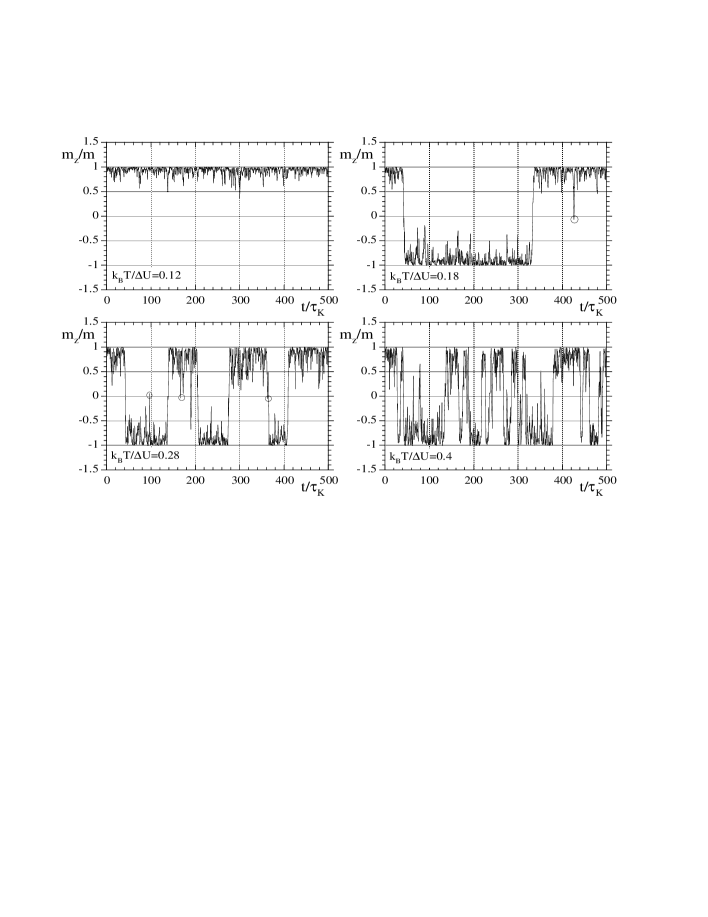
Figure 12: Projection of $\vec{s}(t)$ onto the anisotropy axis for ${\cal H}=-\Delta Us_{z}^{2}$ in zero field, for various temperatures.

The stochastic Landau–Lifshitz equation describes a variety of systems

1. Magnetic systems: magnetic nanoparticles and approximately, magnetic molecular clusters.

2. Electric systems (taking formally the limit $\lambda\gg 1$): permanent dipole molecules, nematic liquid crystals, and relaxor ferroelectrics.

Figure 11 displays the results for the dynamical susceptibility vs. the temperature for an ensemble of 1000 spins with parallel anisotropy axes for $\lambda=0.1$. At low temperatures, the relaxation time obeys $\tau\gg 2\pi/\omega$, so that the probability of over-barrier rotations is almost zero. The spins rotate close to the bottom of the potential wells (see the panel $k_{{\rm B}}T/\Delta U=0.12$ of Fig. 12) and the response is small. As $T$ is increased the spins can depart from the minima (panel $k_{{\rm B}}T/\Delta U=0.18$) and rotate over the barrier. However, since the jump mechanism is not efficient enough, the response lags behind the probing field, and an appreciable imaginary component of the response arises. If $T$ is further increased, the very thermal agitation, which up to this point was responsible for the growth of the response, reaches a level that simultaneously disturbs the alignment of the magnetic moments in the field direction. The response has then a maximum and starts to decrease. Finally, at still higher temperatures the jumps are so frequent (panel $k_{{\rm B}}T/\Delta U=0.4$) that the spins quickly redistribute according to the conditions set by the instantaneous field and the response tends to the thermal equilibrium one.

7.2 Methods for the Fokker–Planck equation

There are several methods to solve Fokker–Planck equations not amenable for an analytical treatment. Among them we can mention the method of the eigenvalues, which consist in finding the eigenvalues of the Fokker–Planck operator occurring in the dynamical equation $\partial_{t}P={\cal L}_{\scriptscriptstyle{\rm FP}}P$ However, the operator ${\cal L}_{\scriptscriptstyle{\rm FP}}$ is not in general Hermitian. If the stationary distribution is known $P_{0}$, and ${\cal L}_{\scriptscriptstyle{\rm FP}}$ fulfills the detailed balance condition, it can be seen that the transformed operator $\overline{{\cal L}}_{\scriptscriptstyle{\rm FP}}=P_{0}^{-1/2}{\cal L}_{\scriptscriptstyle{\rm FP}}P_{0}^{1/2}$ is Hermitian, so the problem can be reduced to an ordinary eigenvalue problem.

$$\overline{{\cal L}}_{\scriptscriptstyle{\rm FP}}p_{n}=-\lambda_{n}p_{n}\;,$$ (7.13)

from which we will have $P(y,t)=\sum_{n}a_{n}p_{n}(y)e^{-\lambda_{n}t}$. However, along with relying on the knowledge of $P_{0}$ and the detailed balance condition, the method has the drawback that the eigenvalue problem may be difficult to solve (as happens for the Schrödinger equation). Concerning approximate methods, we can mention the small noise expansion (also for Langevin equations) and the method of adiabatic elimination of fast variables, which reduces the dimensionality of the problem.

In what follows we shall discuss an alternative method, the continued fraction method, which is a special case of the expansion into complete sets approach. The method, although limited in principle to problems with a few variables, it is exact and in general very efficient, and, in addition, illustrates more general techniques used in non-equilibrium statistical mechanics. We shall discuss the method with two important examples: the Klein–Kramers equation and the Fokker–Planck equation for the Debye dipole.

7.2.1 Solution of the Klein–Kramers equation by continued–fractions

The Klein–Kramers equation (5.20) can be written in the compact form as

$$\partial_{t}P=\Big{(}\underbrace{{\cal L}_{\rm rev}+{\cal L}_{\rm irr}}_{{\cal L}_{\scriptscriptstyle{\rm FP}}}\Big{)}P\;,\qquad\left\{\begin{array}[]{rcl}{\cal L}_{\rm rev}&=&-v\,\partial_{x}+V^{\prime}\partial_{v}=\big{\{}{\cal H}\,,\cdot\big{\}}_{\rm PB}\\[4.30554pt] {\cal L}_{\rm irr}&=&\gamma\,\partial_{v}\left[v+(k_{{\rm B}}T/m)\partial_{v}\right]\end{array}\right.$$ (7.14)

Scaled quantities.

To simplify the notation, we introduce a thermal rescaling of the velocity, time, damping, and potential

$$\bar{v}=v/\sqrt{k_{{\rm B}}T/m}\;,\quad\bar{t}=t\times\sqrt{k_{{\rm B}}T/m}\;,\quad\bar{\gamma}=\gamma/\sqrt{k_{{\rm B}}T/m}\;,\quad U=mV/k_{{\rm B}}T\;.$$ (7.15)

Well, for the $v$, $t$, and $\gamma$ so defined we shall not keep the bars and we shall simply write the Klein–Kramers equation as

$${\framebox{$\displaystyle{\partial_{t}P=\left({\cal L}_{\rm rev}+{\cal L}_{\rm irr}\right)P\;,\qquad\left\{\begin{array}[]{rcl}{\cal L}_{\rm rev}&=&-v\,\partial_{x}+U^{\prime}\partial_{v}\\ {\cal L}_{\rm irr}&=&\gamma\,\partial_{v}\left(v+\partial_{v}\right)\end{array}\right.\;.}$}}$$ (7.16)

Expansion in an orthonormal basis of $v$.

We can expand the probability distribution $P(x,v,t)$ in an orthonormal basis $\psi_{n}(v)$ (to be specified below) as follows

$$P=W\sum_{n}c_{n}(x,t)\psi_{n}(v)\;,$$ (7.17)

where $W=W(x,v)$ is some function we extract for later convenience. Due to the orthonormality of the $\psi_{n}(v)$, we can write $c_{n}=\int\!{\rm d}v\,\psi_{n}P/W$, and hence

$$\mbox{OBS: partial derivatives}\dot{c}_{n}=\int\!{\rm d}v\,\psi_{n}W^{-1}\underbrace{\partial_{t}P}_{{\cal L}_{\scriptscriptstyle{\rm FP}}P}=\int\!{\rm d}v\,\psi_{n}\left(W^{-1}{\cal L}_{\scriptscriptstyle{\rm FP}}W\right)\underbrace{P/W}_{\sum_{m}c_{m}\psi_{m}}\;.$$

Then, we can compactly write

$${\framebox{$\displaystyle{\dot{c}_{n}=\sum_{m}\hat{Q}_{n,m}c_{m}\;,\qquad\hat{Q}_{n,m}=\int\!{\rm d}v\,\psi_{n}\overline{{\cal L}}_{\scriptscriptstyle{\rm FP}}\psi_{m}\quad\overline{{\cal L}}_{\scriptscriptstyle{\rm FP}}=W^{-1}{\cal L}_{\scriptscriptstyle{\rm FP}}W\;.}$}}$$ (7.18)

Then, the equations for the $c_{n}$ are like a system of linear equations with the matrix elements of $\overline{{\cal L}}_{\scriptscriptstyle{\rm FP}}$. However, the $\hat{Q}_{n,m}$ still contain operators over $x$. Besides, it seems that all the $c_{m}$, contribute to the equation for $\dot{c}_{n}$.

As for the function $W$, by analogy with the transformation $P_{0}^{-1/2}{\cal L}_{\scriptscriptstyle{\rm FP}}P_{0}^{1/2}$ to simplify the problem, we try it at least for the $v$ dependent part. Then, since $P_{0}\propto\exp(-v^{2}/2)$ in our units we put $W\propto\exp(-v^{2}/4)$. For the $x$ dependent part, one sets $W\propto\exp(-\varepsilon U)$, which for $\varepsilon=1/2$ corresponds to the $x$-dependent part of $P_{0}^{1/2}$ (if given by the Boltzmann distribution). Thus, from these considerations we set $W\propto\exp[-(v^{2}/4+\varepsilon U)]$.

Calculation of $\overline{{\cal L}}_{\scriptscriptstyle{\rm FP}}=W^{-1}{\cal L}_{\scriptscriptstyle{\rm FP}}W$.

Since ${\cal L}_{\scriptscriptstyle{\rm FP}}={\cal L}_{\rm rev}+{\cal L}_{\rm irr}$, we have to calculate $\overline{\cal L}_{\rm rev}=W^{-1}{\cal L}_{\rm rev}W$ and $\overline{\cal L}_{\rm irr}=W^{-1}{\cal L}_{\rm irr}W$.

For $\overline{\cal L}_{\rm irr}$ we have

$$\gamma^{-1}\overline{\cal L}_{\rm irr}f=e^{v^{2}/4}\partial_{v}\left(v+\partial_{v}\right)e^{-v^{2}/4}f=-\left(-\partial_{v}^{2}+{\textstyle\frac{1}{4}}v^{2}-{\textstyle\frac{1}{2}}\right)f\;,$$

which has the structure of (minus) the Hamilton operator of the harmonic oscillator in quantum mechanics. Hence, we introduce creation and annihilation operators $b^{+}$ and $b$, defined as

$$\left\{\begin{array}[]{lcr}b&=&\partial_{v}+\tfrac{1}{2}v\\[2.15277pt] b^{+}&=&-\partial_{v}+\tfrac{1}{2}v\end{array}\right.\qquad\Longrightarrow\qquad\big{[}b\,,b^{+}\big{]}=1\;.$$ (7.19)

Since the $1/2$ in $\overline{\cal L}_{\rm irr}$ cancels the “zero-point fluctuations”, we finally have

$${\framebox{$\displaystyle{\overline{\cal L}_{\rm irr}=-\gamma b^{+}b\;.}$}}$$ (7.20)

Because of this, it seems natural to choose the $\psi_{n}(v)$ as the Hermite functions

$$\psi_{n}(v)=\frac{1}{\sqrt{n!(2\pi)^{1/2}}}\,e^{-v^{2}/4}H_{n}(v)\;.$$ (7.21)

For $\overline{\cal L}_{\rm rev}$, since ${\cal L}_{\rm rev}=-v\,\partial_{x}+U^{\prime}\partial_{v}$, we need $\overline{\partial_{v}}$ and $\overline{\partial_{x}}$

$$\overline{\partial_{v}}f = e^{v^{2}/4}\partial_{v}\left(e^{-v^{2}/4}f\right)\;,\qquad\Rightarrow\qquad\overline{\partial_{v}}=-b^{+}$$

$$\overline{\partial_{x}}f = e^{\varepsilon U}\partial_{x}\left(e^{-\varepsilon U}f\right)\;,\qquad\Rightarrow\qquad\overline{\partial_{x}}=\partial_{x}-\varepsilon U^{\prime}\;.$$

Then, for $\overline{\cal L}_{\rm rev}$ we have

$$\overline{\cal L}_{\rm rev}=-\underbrace{\left(b+b^{+}\right)}_{v}\underbrace{\left(\partial_{x}-\varepsilon U^{\prime}\right)}_{\overline{\partial_{x}}}\underbrace{-b^{+}}_{\overline{\partial_{v}}}U^{\prime}=-b\left(\partial_{x}-\varepsilon U^{\prime}\right)-b^{+}\left[\partial_{x}+(1\!-\!\varepsilon)U^{\prime}\right]\;.$$

Calling $D_{+}$ to the “coefficient” of $b$ and $D_{-}$ to that of $b^{+}$, we finally have

$$\left\{\begin{array}[]{rcl}D_{+}&=&\partial_{x}-\varepsilon U^{\prime}\\ D_{-}&=&\partial_{x}+(1\!-\!\varepsilon)U^{\prime}\end{array}\right.\quad\Rightarrow\quad{\framebox{$\displaystyle{\overline{\cal L}_{\rm rev}=-bD_{+}-b^{+}D_{-}\;.}$}}$$ (7.22)

Calculation of $\hat{Q}_{n,m}$: the Brinkman hierarchy.

Recall that we need $\overline{{\cal L}}_{\scriptscriptstyle{\rm FP}}=\overline{\cal L}_{\rm rev}+\overline{\cal L}_{\rm irr}$, to obtain its matrix elements $\hat{Q}_{n,m}=\int\!{\rm d}v\,\psi_{n}\overline{{\cal L}}_{\scriptscriptstyle{\rm FP}}\psi_{m}$, which enter in the equation of motion for the coefficients $\dot{c}_{n}=\sum_{m}\hat{Q}_{n,m}c_{m}$. This is an easy task now, since we have written $\overline{\cal L}_{\rm irr}$ and $\overline{\cal L}_{\rm rev}$ in terms of $b$ and $b^{+}$. Then, using the “ladder” properties of $b$ and $b^{+}$, that is, $b^{+}\psi_{n}=\sqrt{n+1}\psi_{n+1}$ and $b\psi_{n}=\sqrt{n}\psi_{n-1}$, plus the orthogonality of the $\psi_{n}$, we obtain

$$\hat{Q}_{n,m}=\int\!{\rm d}v\,\psi_{n}\left(\overline{\cal L}_{\rm rev}+\overline{\cal L}_{\rm irr}\right)\psi_{m}=-\sqrt{n}D_{-}\delta_{n-1,m}-n\gamma\delta_{n,m}-\sqrt{n+1}D_{+}\delta_{n+1,m}\;.$$

Therefore, the sum in $\dot{c}_{n}=\sum_{m}\hat{Q}_{n,m}c_{m}$, is trivially done, and one finally gets the so-called Brinkman hierarchy (1956)

$${\framebox{$\displaystyle{\dot{c}_{n}=-\left(\sqrt{n}D_{-}\,c_{n-1}+\gamma nc_{n}+\sqrt{n+1}D_{+}\,c_{n+1}\right)\;.}$}}$$ (7.23)

We see that, due to (i) the choice of the basis functions to expand $P$ and (ii) the extraction of the factor $\exp(-v^{2}/4)$, only the nearest neighbours of $c_{n}$ contribute in $\dot{c}_{n}=\sum_{m}\hat{Q}_{n,m}c_{m}$. Writing explicitly the equations, we see that this fact results in a tri-diagonal structure of the system

$${\framebox{$\displaystyle{\begin{array}[]{ccccccccccc}-\dot{c}_{0}&=&0\gamma c_{0}&+&\sqrt{1}\,D_{+}c_{1}&+&0&+&\cdots&&\\[6.45831pt] -\dot{c}_{1}&=&\sqrt{1}\,D_{-}c_{0}&+&1\gamma c_{1}&+&\sqrt{2}\,D_{+}c_{2}&+&0&+&\cdots\\[6.45831pt] -\dot{c}_{2}&=&0&+&\sqrt{2}\,D_{-}c_{1}&+&2\gamma c_{2}&+&\sqrt{3}\,D_{+}c_{3}&+&0\\[6.45831pt] -\dot{c}_{3}&=&\cdots&+&0&+&\sqrt{3}\,D_{-}c_{2}&+&3\gamma c_{3}&+&\sqrt{4}\,D_{+}c_{4}\\[6.45831pt] \vdots&&\vdots&&\vdots&&\vdots&&\vdots&&\vdots\end{array}}$}}$$

This equation is completely equivalent to the Klein–Kramers equation (7.16) and valid for any potential.

Continued fractions.

Why are we so happy for having transformed the Klein–Kramers equation into an infinity hierarchy for the $c_{n}$? First, by taking the Laplace transform $\tilde{f}(s)\equiv\int_{0}^{\infty}{{\rm d}t}\,e^{-st}f(t)$ a differential-recurrence relation of the general form

$$\frac{{\rm d}c_{i}}{{\rm d}t}+Q_{i}^{-}c_{i-1}+Q_{i}c_{i}+Q_{i}^{+}c_{i+1}=f_{i}\;,$$ (7.24)

can be reduced to (we omit the tildes on the Laplace transforms)

$${\framebox{$\displaystyle{Q_{i}^{-}c_{i-1}+\hat{Q}_{i}c_{i}+Q_{i}^{+}c_{i+1}=\hat{f}_{i}\;,}$}}$$ (7.25)

where $\hat{Q}_{i}=Q_{i}+s$ and $\hat{f_{i}}=f_{i}+c_{i}(0)$. Then, this relation can be solved by introducing the ansatz $c_{i}=S_{i}c_{i-1}+a_{i}$, obtaining

$${\framebox{$\displaystyle{c_{i}=S_{i}c_{i-1}+a_{i}\quad\mbox{with}\quad S_{i}=-\frac{Q_{i}^{-}}{\hat{Q}_{i}+Q_{i}^{+}S_{i+1}}\quad a_{i}=-\frac{Q_{i}^{+}a_{i+1}-\hat{f}_{i}}{\hat{Q}_{i}+Q_{i}^{+}S_{i+1}}}$}}$$ (7.26)

It is to be remarked that the quantities involved in the relation (7.25) do not need to be scalars, but they can be vectors ($c_{i}$ and $f_{i}$) and the coefficients $Q_{i}$ matrices. The only change in the solution (7.26) is that the fraction bar then means matrix inversion.

The reason for the name “continued fraction”, is that, if we consider for instance $S_{i}$, it is given in terms of $S_{i+1}$ in the denominator. But this can be expressed in terms of $S_{i+2}$, and so on, leading to an expression of the form

$$K=\cfrac{p_{1}}{q_{1}+\cfrac{p_{2}}{q_{2}+\cfrac{p_{3}}{q_{3}+\dotsb}}}\;,$$ (7.27)

which is called a continued fraction. Well, if the $c_{i}$ are judiciously chosen to decrease with increasing $i$, we can truncate at some large $N$, setting $c_{N}=0$. This leads all the quantities to vanish at $i=N$, and we can iterate downward the continued fractions in Eq. (7.26) down to $i=0$, storing the successive $S_{i}$ and $a_{i}$. Then, starting from $c_{0}$ (usually known by some means, e.g., normalisation of the distribution), we iterate upwards with $c_{i}=S_{i}c_{i-1}+a_{i}$, obtaining the solution to the recurrence-relation (7.25). To ensure convergence, one can repeat the calculation with a truncation index $2N$, $4N$, etc. and check that the results do not change. Note that the steps described above are very easy to code in a computer program (even in a programmable pocket calculator). This is the answer to the question of why it was important to transform the Klein–Kramers equation into the Brinkman hierarchy.

Solving the Brinkman hierarchy.

As written, the hierarchy (7.23), involves coefficients that still contain the operators $D_{\pm}$ over the $x$ variables, instead of true coefficients. But we only need to find a representation of those operators in a basis of functions of $x$, say $u_{p}(x)$. Then we just calculate the matrix elements of any operator $\hat{A}$ in that basis $A_{p\,q}=\int\!{\rm d}x\,u_{p}^{\ast}\hat{A}u_{q}$, while the expansion coefficients of $c_{n}(x,t)$ are expressed as a column vector

$$c_{n}(x,t)=\sum_{p}c_{n}^{p}(t)u_{p}(x)\;,\qquad\Rightarrow\qquad{\bf C}_{n}=\left(\begin{array}[]{c}c_{n}^{-P}\\ \vdots\\ c_{n}^{P}\end{array}\right)\;.$$

Then, the Brinkman hierarchy (7.23) is reduced to the following differential recurrence relation

$${\framebox{$\displaystyle{\dot{{\bf C}}_{n}={\bf Q}_{n}^{-}{\bf C}_{n-1}+{\bf Q}_{n}{\bf C}_{n}+{\bf Q}_{n}^{+}{\bf C}_{n+1}\;,}$}}$$ (7.28)

whose coefficients are not any more operators but ordinary matrices, with elements

$$\begin{array}[]{ccl}\left({\bf Q}_{n}^{-}\right)_{p\,q}&=&-\sqrt{n}\left[\left(\partial_{x}\right)_{p\,q}+(1\!-\!\varepsilon)U_{p\,q}^{\prime}\right]\\ \left({\bf Q}_{n}\right)_{p\,q}&=&-n\,\gamma\,\delta_{p\,q}\\ \left({\bf Q}_{n}^{+}\right)_{p\,q}&=&-\sqrt{n+1}\left[\left(\partial_{x}\right)_{p\,q}-\varepsilon U_{p\,q}^{\prime}\right]\end{array}$$ (7.29)

The choice of the basis functions $u_{p}(x)$ is naturally dictated by the symmetry of the potential.

In this form, we can directly use the method of continued fractions to solve the Brinkman hierarchy. In principle, with the $c_{n}^{p}$ obtained we can construct the probability distribution and compute any observable. Nevertheless, this is not even required, since common observables are directly obtained from the expansion coefficients. For instance, if $\varepsilon=0$ in $W\propto\exp(-v^{2}/4)$, this quantity is after normalisation $W=\psi_{0}$ (see the definition of the Hermite functions (7.21)] so that for the averaged velocity $\left\langle v\right\rangle=\int\!{\rm d}x\,\int\!{\rm d}v\,vP(x,v,t)$ we get

$$\left\langle v\right\rangle=\sum_{n\,p}c_{n}^{p}\int\!{\rm d}x\,u_{p}(x)\underbrace{\int\!{\rm d}v\,\overbrace{\underbrace{v}_{b+b^{+}}\psi_{0}(v)}^{\psi_{1}}\psi_{n}(v)}_{\delta_{n,1}}=\sum_{p}c_{1}^{p}\int\!{\rm d}x\,u_{p}(x)=c_{1}^{0}\;,$$

where he have just assumed that the $0$th element of the basis $u_{p}(x)$ is constant (say $u_{0}=1$), so that the result follows from orthogonality ($u_{0}\perp u_{n}$).

Example: particles in a periodic potential.

Let us consider the case of a general periodic potential $U^{\prime}=\sum_{q}U_{q}^{\prime}e^{\mathrm{i}qx}$, where the $U_{q}^{\prime}$ are the Fourier components of the potential derivative. In this case the natural choice of the basis functions $u_{p}(x)$ is that of plane waves $u_{p}(x)=e^{\mathrm{i}qx}/\sqrt{2\pi}$. Then the matrix elements needed to construct the matrices ${\bf Q}_{n}$ in Eq. (7.29) are simply

$$\left(\partial_{x}\right)_{p\,q}=\mathrm{i}p\delta_{p\,q}\;,\qquad(U^{\prime})_{p\,q}=U_{p-q}^{\prime}\;.$$ (7.30)

Then, the number of diagonals occupied in the matrices ${\bf Q}_{n}$ below and above the main diagonal is equal to the number of harmonics in the potential. In the example of the cosine potential, this number is only one, while in the ratchet potential (7.8), this number is two.

Well, in the example of the ratchet potential we computed the average velocity vs. force by Langevin simulation (Fig. 10). If we compute now the same curves with the continued-fraction method, we get a complete agreement shown in Fig. 13 (without any free parameter).

Figure 13: Depinning curves in a ratchet potential of Fig. 10, obtained with Langevin simulation (symbols), together with the results obtained with the continued-fraction method (thick lines).

As an additional example, in Fig. 14, we show the real part of the dynamical susceptibility as a function of the frequency in an ordinary (non-ratchet) periodic potential (thus, the curves could correspond to a Josephson junction, or to the ac conductivity in a transport problem). We see a peak about the frequency of oscillations in the bottom of the potential wells (which defines the frequency scale in the graph). The peak becomes more and more sharp and high the lower the damping is, showing the typical features of a resonant system.

Figure 14: Real part of the dynamical susceptibility (ac conductivity) vs. frequency. The curves have been obtained with the continued-fraction method for $T/d=0.1$ and various values of the damping $\gamma=1$, $0.3$, $0.1$, $0.03$. The resonance at $\omega\sim 1$ is clearly seen.

When the continued-fraction method can be used its advantages are: (i) it has no statistical error bars, (ii) it is in general extremely efficient, (iii) it outputs the complete distribution if required, and (iv) it may be extended to problems of quantum Brownian motion. The drawbacks are that it is quite specific of the problem to be solved (we need to compute the matrix elements for each potential, and the relation between the coefficients and the observables), and in this respect the Langevin simulations do not have this problem. Besides, the simulations output trajectories, which are lost in the continued fraction approach. Finally, it can only be implemented for systems with a few variables (e.g., independent particles), while the Langevin simulations do not suffer this limitation.

7.2.2 Solution of the Debye equation by continued–fractions

This continued-fraction method can also be applied to rotational problems. We shall illustrate this with the Fokker–Planck equation for a dipole (4.30). First, using the definition of the Debye relaxation time $\tau_{{\rm D}}=\zeta/2k_{{\rm B}}T$ [Eq. (5.35)], the abbreviation $\alpha=pE/k_{{\rm B}}T$ and changing to Cartesian coordinates $z=\cos\vartheta$, the Debye equation can be written as

$${\framebox{$\displaystyle{2\tau_{{\rm D}}\frac{\partial P}{\partial t}=\frac{\partial}{\partial z}\left[(1-z^{2})\left(\frac{\partial P}{\partial z}-\alpha\,P\right)\right]\;.}$}}$$ (7.31)

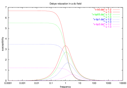
Figure 15: Dynamical susceptibility (polarisability) of a dipole in various static fields. The curves have been obtained with the continued-fraction method for $T=0.1$ and the fields used are $pE/k_{{\rm B}}T=0$, $1$, $2$ and $4$.

In this problem the natural choice for basis function is the Legendre polynomials $p_{n}(\cos\vartheta)$ [cf. Eq. (7.17)]

$$P=\sum_{n}c_{n}(t)p_{n}(z)\;.$$ (7.32)

Due to the orthogonality of the $p_{n}(z)$, $\int_{-1}^{1}\!{\rm d}z\,p_{n}(z)p_{m}(z)=2\delta_{n,m}/(2n+1)$, we have $c_{n}=[(2n+1)/2]\int\!{\rm d}z\,p_{n}(z)\,P(z)$. Then the equation of motion for the $c_{n}$ reads [cf. Eq. (7.18)]

$$\frac{4\tau_{{\rm D}}}{2n+1}\dot{c}_{n}=\int\!{\rm d}z\,p_{n}\overbrace{{\cal L}_{\scriptscriptstyle{\rm FP}}\underbrace{P}_{\hbox to0.0pt{$\displaystyle\scriptstyle\sum_{m}c_{m}p_{m}$\hss}}}^{\partial_{t}P}=\sum_{m}\hat{Q}_{n,m}c_{m}\;,\quad\mbox{with}\quad Q_{n,m}=\int\!{\rm d}z\,p_{n}{\cal L}_{\scriptscriptstyle{\rm FP}}p_{m}\;.$$

To calculate $Q_{n,m}$ (which is not an operator here), we use relations obeyed by the Legendre polynomials and an integration by parts:

$$Q_{n,m} = \int\!{\rm d}z\,p_{n}\frac{{\rm d}}{{\rm d}z}\left[(1-z^{2})\left(\frac{{\rm d}p_{m}}{{\rm d}z}-\alpha\,p_{m}\right)\right]$$

$$= -m(m+1)\int\!{\rm d}z\,p_{n}p_{m}+\alpha\int\!{\rm d}z\,\frac{{\rm d}p_{n}}{{\rm d}z}(1-z^{2})p_{m}$$

$$= -n(n+1)\frac{2\delta_{nm}}{2n+1}+\alpha\,\frac{n(n+1)}{2n+1}\left(\frac{2\delta_{n-1,m}}{2n-1}-\frac{2\delta_{n+1,m}}{2n+3}\right)\;.$$

Inserting this result into the equation for $\dot{c}_{n}$, we finally find

$${\framebox{$\displaystyle{\frac{2\tau_{{\rm D}}}{n(n+1)}\dot{c}_{n}=-c_{n}+\frac{pE}{k_{{\rm B}}T}\left(\frac{c_{n-1}}{2n-1}-\frac{c_{n+1}}{2n+3}\right)\;.}$}}$$ (7.33)

which is a tridiagonal differential-recurrence relation for the dipole analogous to the Brinkman hierarchy (7.23).

Solving Eq. (7.33) by continued fractions, we can obtain any observable. For instance, we can compute the linear susceptibility in a static field (remember that the solved this problem in the absence of bias field), by setting $E=E_{0}+\Delta E\cos(\omega t)$. The results are shown in Fig. 15, for various $E_{0}$. It is seen that the equilibrium susceptibility (real part at $\omega\to 0$) decreases with $E_{0}$, since the susceptibility measures the slope of the static polarization, which saturates at large fields. Besides the relaxation time (roughly, the inverse of the location of the maximum of the imaginary part) decreases with $E_{0}$, so that the relaxation is faster in a static field.

8 Derivation of Langevin equations in
the bath-of-oscillators formalism

Now we shall discuss the foundations of the Langevin equations by showing how they can be “derived” from more or less microscopic description of a system coupled with its environment.

8.1 Dynamical approaches to the Langevin equations

The Langevin equations we have discussed for Brownian particles and spins, are phenomenological inasmuch as they constructed by augmenting known phenomenological equations by fluctuating terms. For subsequent reference, let us first rewrite these equations in the notation we shall employ later:

$\bullet$ Brownian particle

$$\left\{\begin{array}[]{rcl}\displaystyle\frac{{\rm d}q}{{\rm d}t}&=&\displaystyle\frac{p}{m}\\[8.61108pt] \displaystyle\frac{1}{m}\frac{{\rm d}p}{{\rm d}t}&=&\displaystyle-\frac{\partial V}{\partial q}-\gamma\,\frac{{\rm d}q}{{\rm d}t}+\xi(t)\;,\qquad\left\langle\xi(t)\xi(t^{\prime})\right\rangle=2(\gamma k_{{\rm B}}T/m)\delta(t-t^{\prime})\;.\end{array}\right.$$ (8.1)

Note that the fluctuating terms only enter in the equation for the momentum.

$\bullet$ Brownian spins and dipoles

$$\frac{{\rm d}\vec{s}}{{\rm d}t}=\vec{s}\wedge\left[\vec{B}+\vec{\xi}(t)\right]-\lambda\,\vec{s}\wedge\left(\vec{s}\wedge\vec{B}\right)\;,\quad\left\langle\xi_{k}(t)\xi_{\ell}(t^{\prime})\right\rangle=2(\lambda k_{{\rm B}}T)\delta_{k\ell}\delta(t-t^{\prime})\;.$$ (8.2)

This stochastic Landau–Lifshitz equation is equivalent to the Gilbert equation where the damping term is $\propto-\lambda\vec{s}\wedge({\rm d}\vec{s}/{\rm d}t)$. Recall that Eq. (8.2) contains as a special case the stochastic dynamical equation for the electrical dipole.

Note that in both equations the fluctuating and dissipation terms are not independent: $D=\gamma k_{{\rm B}}T/m$ for the particle, which corresponds to $D=\lambda k_{{\rm B}}T$ for the spin. Besides, the force $F=-\partial V/\partial q$, corresponds to $\vec{B}=-\partial{\cal H}/\partial\vec{s}$, while the damping $-\gamma({\rm d}q/{\rm d}t)$, corresponds to $-\lambda\vec{s}\wedge\left(\vec{s}\wedge\vec{B}\right)$, which as mentioned above is related with $\propto-\lambda\vec{s}\wedge({\rm d}\vec{s}/{\rm d}t)$.

There have been several attempts to justify, starting from dynamical descriptions of a system coupled to its surroundings, these important Langevin equations. The effort was first directed to the Langevin equations for the Brownian particle (translational problems) and then to rotational Brownian motion of spins and dipoles.

In most of those studies, the environment is represented as a set of independent harmonic oscillators. The oscillators are somehow “projected out” and an equation for the system variables is derived. The final equation has the form of a generalized Langevin equation (i.e., containing “memory” terms), whose fluctuating and dissipative terms naturally obey fluctuation-dissipation relations. For instance, for the particle problem one gets

$$\frac{{\rm d}p}{{\rm d}t}=-\frac{\partial{\cal H}}{\partial q}+f(t)-\int_{t_{0}}^{t}\!\!{\rm d}{t^{\prime}}\,{\cal K}(t-t^{\prime})\frac{{\rm d}q}{{\rm d}t}(t^{\prime})\;,\qquad\left\langle f(t)f(t^{\prime})\right\rangle=k_{{\rm B}}T\,{\cal K}(t-t^{\prime})\;.$$ (8.3)

Thus the relaxation (damping) term, involves a memory integral taken along the past history of the system. Besides, the memory kernel ${\cal K}(t-t^{\prime})$ is determined by the correlation properties of the fluctuating force $f(t)$. Thus, if the autocorrelation of the fluctuating terms is very short $\left\langle f(t)f(t^{\prime})\right\rangle\propto\delta(t-t^{\prime})$, the damping term reduces to minus the velocity $-({\rm d}q/{\rm d}t)$ of the particle. Similar results are obtained for the spin and dipole problems.

In what follows we shall discuss the bath of oscillators formalism. First, since we shall use a Hamiltonian formalism throughout, we shall start with a brief review of the main results from Hamiltonian mechanics that we shall need. Subsequently, we shall introduce the model for the system coupled with its environment, deduce the corresponding dynamical equations, and finally discuss some examples.

8.2 Quick review of Hamiltonian dynamics

The dynamical equations for a system with Hamiltonian ${\cal H}(p,q)$ are

$$\frac{{\rm d}q}{{\rm d}t}=\frac{\partial{\cal H}}{\partial p}\;,\qquad\frac{{\rm d}p}{{\rm d}t}=-\frac{\partial{\cal H}}{\partial q}\;.$$ (8.4)

Then, the time evolution of an arbitrary dynamical variable of the system $A(p,q)$ (assumed not explicitly time dependent), is ${\rm d}A/{\rm d}t=(\partial A/\partial q)({\rm d}q/{\rm d}t)+(\partial A/\partial p)({\rm d}p/{\rm d}t)$. Then, using for ${\rm d}q/{\rm d}t$ and ${\rm d}p/{\rm d}t$ the Hamilton equations and introducing the Poisson bracket of two arbitrary dynamical variables

$$\big{\{}A,B\big{\}}\equiv\frac{\partial A}{\partial q}\frac{\partial B}{\partial p}-\frac{\partial A}{\partial p}\frac{\partial B}{\partial q}\;,$$ (8.5)

we have for ${\rm d}A/{\rm d}t$ the basic Hamiltonian evolution equation

$${\framebox{$\displaystyle{\frac{{\rm d}A}{{\rm d}t}=\big{\{}A,{\cal H}\big{\}}\;.}$}}$$ (8.6)

Finally, by using this equation for $A=q$, with $\partial q/\partial q=1$, $\partial q/\partial p=0$, and for $A=p$ with $\partial p/\partial q=0$, and $\partial p/\partial p=1$, we see that the Hamilton equations (8.4) are a particular case of Eq. (8.6). For a system with variables $(p_{a},q_{a})$ $a=1,\dots,N$, the above results are the same, with the only change of introducing a sum over $a$ in the definition of the Poisson bracket.

Two more results we shall need are the product rule of the Poisson bracket

$$\big{\{}A,BC\big{\}}=\big{\{}A,B\big{\}}C+B\big{\{}A,C\big{\}}\;,$$ (8.7)

and the chain rule

$$\big{\{}f,g\big{\}}=\sum_{i,k}\frac{\partial f}{\partial x_{i}}\frac{\partial g}{\partial x_{k}}\big{\{}x_{i},x_{k}\big{\}}\;,\qquad x_{i}=x_{i}(p,q)\;,$$ (8.8)

which immediately follow from the ordinary differentiation rules.

Spin dynamics case.

The equations for an isolated classical spin (not subjected to fluctuations and dissipation)

$$\frac{{\rm d}\vec{s}}{{\rm d}t}=\vec{s}\wedge\vec{B}\;,\qquad\vec{B}=-\frac{\partial{\cal H}}{\partial\vec{s}}\;.$$ (8.9)

can also be written in Hamiltonian form. To this end, let us write the formula for the gradient operator in spherical coordinates

$$\frac{\partial u}{\partial\vec{s}}=\hat{s}\frac{\partial u}{\partial s}+\hat{\vartheta}\frac{1}{s}\frac{\partial u}{\partial\vartheta}+\hat{\varphi}\frac{1}{s\sin\vartheta}\frac{\partial u}{\partial\varphi}\;,$$ (8.10)

where $\varphi$ and $\vartheta$ are the azimuthal and polar angles of $\vec{s}$. Since the length of $\vec{s}$ is constant, the set vectorial equations (8.9), can be written as

$$\frac{{\rm d}\varphi}{{\rm d}t}=-\frac{1}{s\sin\vartheta}\frac{\partial{\cal H}}{\partial\vartheta}\;,\qquad\frac{{\rm d}\vartheta}{{\rm d}t}=\frac{1}{s\sin\vartheta}\frac{\partial{\cal H}}{\partial\varphi}\;,$$ (8.11)

which correspond to the Hamilton equations (8.4) with the conjugate canonical variables

$${\framebox{$\displaystyle{q=\varphi\;,\qquad p=s_{z}\;.}$}}$$ (8.12)

In terms of the variables (8.12) the Cartesian components of the spin are given by

$$s_{x}=\sqrt{s^{2}-p^{2}}\cos q\;,\qquad s_{y}=\sqrt{s^{2}-p^{2}}\sin q\;,\qquad s_{z}=p\;.$$

From these $s_{i}(p,q)$ and the definition of the Poisson bracket of two arbitrary dynamical variables [Eq. (8.5)], one can readily obtain the customary Poisson-bracket (“commutation”) relations among the spin variables

$$\big{\{}s_{i},s_{j}\big{\}}=\sum_{k}\epsilon_{ijk}s_{k}\;,$$ (8.13)

where $\epsilon_{ijk}$ is the Levi–Civita symbol. In addition, on using the chain rule of the Poisson bracket [Eq. (8.8)], one gets the useful relation

$$\big{\{}s_{i},W(\vec{s})\big{\}}=-\bigg{(}\vec{s}\wedge\frac{\partial W}{\partial\vec{s}}\bigg{)}_{i}\;,$$ (8.14)

which is valid for any function of the spin variables $W(\vec{s})$.

8.3 Dynamical equations in the bath-of-oscillators formalism

We shall now study a classical system surrounded by an environment that can be represented by a set of independent classical harmonic oscillators. In spite of its academic appearance, those oscillators could correspond to the normal modes of an electromagnetic field, the lattice vibrations of a crystal (in the harmonic approximation), or they can be an effective low-energy description of a more general surrounding medium (Caldeira and Leggett, [1]).

8.3.1 The system-environment Hamiltonian

The total system consisting of the “system of interest” plus the oscillators representing the environment forms a closed dynamical system that we shall describe by augmenting the isolated-system Hamiltonian as follows

$${\cal H}_{\rm T}={\cal H}(p,q)+\sum_{\alpha}\tfrac{1}{2}\Big{\{}P_{\alpha}^{2}+\omega_{\alpha}^{2}\Big{[}Q_{\alpha}+\frac{\varepsilon}{\omega_{\alpha}^{2}}F_{\alpha}(p,q)\Big{]}^{2}\Big{\}}\;.$$ (8.15)

Here, $\alpha$ is an oscillator index [e.g., the pair $(\vec{k},s)$ formed by the wave-vector and branch index of a normal mode of the environment], and the coupling terms $F_{\alpha}(p,q)$ are arbitrary functions of the system variables. These terms may depend on the parameters of the oscillators $\omega_{\alpha},$ but not on their dynamical variables $P_{\alpha},Q_{\alpha}$. On the other hand, we have introduced a system-environment coupling constant $\varepsilon$ for the sake of convenience in keeping track of the orders of the various contributions.

The terms proportional to $F_{\alpha}^{2}$, which emerge when squaring $Q_{\alpha}+(\varepsilon/\omega_{\alpha}^{2})F_{\alpha}$, are “counter-terms” introduced to balance the coupling-induced renormalization of the Hamiltonian of the system. The formalism takes as previously considered whether such a renormalization actually occurs for a given interaction, so that ${\cal H}$ would already include it (whenever exists). An advantage of this convention is that one deals with the experimentally accessible energy of the system, instead of the “bare” one, which might be difficult to determine.

8.3.2 Dynamical equations

Let us first cast the Hamiltonian (8.15) into the form

$${\cal H}_{\rm T}={\cal H}^{({\rm m})}(p,q)+\sum_{\alpha}\tfrac{1}{2}\left(P_{\alpha}^{2}+\omega_{\alpha}^{2}Q_{\alpha}^{2}\right)+\varepsilon\sum_{\alpha}Q_{\alpha}F_{\alpha}(p,q)\;,$$ (8.16)

where $q$ and $p$ are the canonical coordinate and conjugate momentum of a system with Hamiltonian ${\cal H}(p,q)$ and the “modified” system Hamiltonian ${\cal H}^{({\rm m})}$ augments ${\cal H}$ by the aforementioned counter-terms

$${\cal H}^{({\rm m})}={\cal H}+\frac{\varepsilon^{2}}{2}\sum_{\alpha}\frac{F_{\alpha}^{2}}{\omega_{\alpha}^{2}}\;.$$ (8.17)

Besides, in the above expression for ${\cal H}_{\rm T}$ the Hamiltonian of the oscillators is clearly recognised ${\cal H}_{{\rm E}}=\sum_{\alpha}\tfrac{1}{2}\left(P_{\alpha}^{2}+\omega_{\alpha}^{2}Q_{\alpha}^{2}\right)$, and the same for the coupling term ${\cal H}_{{\rm int}}=\varepsilon\sum_{\alpha}Q_{\alpha}F_{\alpha}(p,q)$.

The equation of motion for any dynamical variable $C$ without explicit dependence on the time, $\partial C/\partial t\equiv 0$, is given by the basic Hamiltonian evolution equation (8.6) with ${\cal H}\to{\cal H}_{\rm T}$, with the whole Poisson bracket is given by

$$\big{\{}A,B\big{\}}\equiv\frac{\partial A}{\partial q}\frac{\partial B}{\partial p}-\frac{\partial A}{\partial p}\frac{\partial B}{\partial q}+\sum_{\alpha}\frac{\partial A}{\partial Q_{\alpha}}\frac{\partial B}{\partial P_{\alpha}}-\frac{\partial A}{\partial P_{\alpha}}\frac{\partial B}{\partial Q_{\alpha}}\;.$$

Therefore, the (coupled) equations of motion for any dynamical variable of the system $A(p,q)$ and the environment variables read ($C=A,P_{\alpha}$, and $Q_{\alpha}$)

$$\frac{{\rm d}A}{{\rm d}t} = \big{\{}A,{\cal H}^{({\rm m})}\big{\}}+\varepsilon\sum_{\alpha}Q_{\alpha}\big{\{}A,F_{\alpha}\big{\}}\;,$$ (8.18)

$$\frac{{\rm d}Q_{\alpha}}{{\rm d}t} = P_{\alpha}\;,\qquad\frac{{\rm d}P_{\alpha}}{{\rm d}t}=-\omega_{\alpha}^{2}Q_{\alpha}-\varepsilon F_{\alpha}\;,$$ (8.19)

where we have used $\big{\{}Q_{\alpha},P_{\alpha}\big{\}}=1$. The goal is to derive a dynamical equation for $A(p,q)$ involving the system variables only (reduced dynamical equation).

On considering that in Eqs. (8.19) the term $-\varepsilon F_{\alpha}(t)=-\varepsilon F_{\alpha}[p(t),q(t)]$ plays the rôle of a time-dependent forcing on the oscillators, those equations can be explicitly integrated, yielding

$$Q_{\alpha}(t)=Q_{\alpha}^{{\rm h}}(t)-\frac{\varepsilon}{\omega_{\alpha}}\int_{t_{0}}^{t}\!\!{\rm d}{t^{\prime}}\,\sin[\omega_{\alpha}(t-t^{\prime})]F_{\alpha}(t^{\prime})\;,$$ (8.20)

where

$$Q_{\alpha}^{{\rm h}}(t)=Q_{\alpha}(t_{0})\cos[\omega_{\alpha}(t-t_{0})]+[P_{\alpha}(t_{0})/\omega_{\alpha}]\sin[\omega_{\alpha}(t-t_{0})]\;,$$ (8.21)

are the solutions of the homogeneous system of equations for the oscillators in the absence of the system-environment interaction (proper modes of the environment). Then, on integrating by parts in Eq. (8.20) one gets for the combination $\varepsilon Q_{\alpha}$ that appears in Eq. (8.18)

$$\varepsilon Q_{\alpha}(t)=f_{\alpha}(t)-\left[{\cal K}_{\alpha}(t-t^{\prime})F_{\alpha}(t^{\prime})\right]_{t^{\prime}=t_{0}}^{t^{\prime}=t}+\int_{t_{0}}^{t}\!\!{\rm d}{t^{\prime}}\,{\cal K}_{\alpha}(t-t^{\prime})\frac{{\rm d}F_{\alpha}}{{\rm d}t}(t^{\prime})\;,$$ (8.22)

where

$$f_{\alpha}(t)=\varepsilon Q_{\alpha}^{{\rm h}}(t)\;,\qquad{\cal K}_{\alpha}(\tau)=\frac{\varepsilon^{2}}{\omega_{\alpha}^{2}}\cos(\omega_{\alpha}\tau)\;.$$ (8.23)

Next, in order to eliminate the environment variables from the equation for $A(p,q)$, one substitutes Eq. (8.22) back into Eq. (8.18), getting

$$\frac{{\rm d}A}{{\rm d}t}=\big{\{}A,{\cal H}^{({\rm m})}\big{\}} - \sum_{\alpha}\big{\{}A,F_{\alpha}\big{\}}{\cal K}_{\alpha}(0)F_{\alpha}(t)+\sum_{\alpha}\big{\{}A,F_{\alpha}\big{\}}{\cal K}_{\alpha}(t-t_{0})F_{\alpha}(t_{0})$$

$$+ \sum_{\alpha}\big{\{}A,F_{\alpha}\big{\}}\bigg{[}f_{\alpha}(t)+\int_{t_{0}}^{t}\!\!{\rm d}{t^{\prime}}\,{\cal K}_{\alpha}(t-t^{\prime})\frac{{\rm d}F_{\alpha}}{{\rm d}t}(t^{\prime})\bigg{]}\;.$$

The term $\sum_{\alpha}\big{\{}A,F_{\alpha}\big{\}}{\cal K}_{\alpha}(t-t_{0})F_{\alpha}(t_{0})$ depends on the initial state of the system $(p(t_{0}),q(t_{0}))$ and produces a transient response that can be ignored in the long-time dynamics (we shall return to this question below). The parallel term $-\sum_{\alpha}\big{\{}A,F_{\alpha}\big{\}}{\cal K}_{\alpha}(0)F_{\alpha}(t)$ is derivable from a Hamiltonian and balances exactly the term due to the counter-terms in $\big{\{}A,{\cal H}^{({\rm m})}\big{\}}$. This can be shown by using

$$-\sum_{\alpha}\big{\{}A,F_{\alpha}\big{\}}{\cal K}_{\alpha}(0)F_{\alpha}=\big{\{}A,-\tfrac{1}{2}\sum_{\alpha}{\cal K}_{\alpha}(0)F_{\alpha}^{2}\big{\}}\;,$$

which follows from the product rule (8.7) of the Poisson bracket and then using ${\cal K}_{\alpha}(0)=\varepsilon^{2}/\omega_{\alpha}^{2}$ [see Eq. (8.23)]. Therefore, one is left with the reduced dynamical equation

$$\frac{{\rm d}A}{{\rm d}t}=\big{\{}A,{\cal H}\big{\}}+\sum_{\alpha}\big{\{}A,F_{\alpha}\big{\}}\bigg{[}f_{\alpha}(t)+\int_{t_{0}}^{t}\!\!{\rm d}{t^{\prime}}\,{\cal K}_{\alpha}(t-t^{\prime})\frac{{\rm d}F_{\alpha}}{{\rm d}t}(t^{\prime})\bigg{]}\;,$$ (8.24)

where the first term yields the free (conservative) time evolution of the system, whereas the second term incorporates the effects of the interaction of the system with its environment.

To conclude, let us decompose the coupling functions as

$$F_{\alpha}(p,q)=\sum_{{\rm a}}c_{\alpha}^{{\rm a}}W_{{\rm a}}(p,q)\;.$$ (8.25)

Here “${\rm a}$” stands for a general index depending on the type of interaction. The idea is to split the part of the coupling $W_{{\rm a}}(p,q)$ which is common to all the modes, so that $F_{\alpha}$ is obtained multiplying that part by certain mode-dependent system-environment coupling constants $c_{\alpha}^{{\rm a}}$. For instance, if $\alpha$ is a mode of wave-vector $\vec{k}$, and $F_{\vec{k}}=\vec{k}\cdot\vec{r}$, then ${\rm a}=i$ (the Cartesian index) with $c_{\vec{k}}^{i}=k_{i}$ and $W_{i}=r_{i}$. Introducing the above coupling function into Eq. (8.24), we have

$$\frac{{\rm d}A}{{\rm d}t}=\big{\{}A,{\cal H}\big{\}}+\sum_{\alpha}\big{\{}A,\sum_{{\rm a}}c_{\alpha}^{{\rm a}}W_{{\rm a}}\big{\}}\bigg{[}f_{\alpha}(t)+\int_{t_{0}}^{t}\!\!{\rm d}{t^{\prime}}\,{\cal K}_{\alpha}(t-t^{\prime})\sum_{{\rm b}}c_{\alpha}^{{\rm b}}\frac{{\rm d}W_{{\rm b}}}{{\rm d}t}(t^{\prime})\bigg{]}\;.$$

Therefore, we finally have

$${\framebox{$\displaystyle{\frac{{\rm d}A}{{\rm d}t}=\big{\{}A,{\cal H}\big{\}}+\sum_{{\rm a}}\big{\{}A,W_{{\rm a}}\big{\}}\bigg{[}f_{{\rm a}}(t)+\int_{t_{0}}^{t}\!\!{\rm d}{t^{\prime}}\,\sum_{{\rm b}}{\cal K}_{{\rm a}{\rm b}}(t-t^{\prime})\frac{{\rm d}W_{{\rm b}}}{{\rm d}t}(t^{\prime})\bigg{]}}$}}$$ (8.26)

where

$${\framebox{$\displaystyle{f_{{\rm a}}(t)=\sum_{\alpha}c_{\alpha}^{{\rm a}}f_{\alpha}(t)\;,\qquad{\cal K}_{{\rm a}{\rm b}}(\tau)=\sum_{\alpha}c_{\alpha}^{{\rm a}}c_{\alpha}^{{\rm b}}{\cal K}_{\alpha}(\tau)\;.}$}}$$ (8.27)

The terms $f_{{\rm a}}(t)$ are customarily interpreted as fluctuating “forces” (or “fields”). Indeed $f_{{\rm a}}(t)$ is a sum of a large number of sinusoidal terms with different frequencies and phases; this can give to $f_{{\rm a}}(t)$ the form of a highly irregular function of $t$ that is expected for a fluctuating term (see below). The integral term keeps in general memory of the previous history of the system, and provides the relaxation due to the interaction with the surrounding medium.

The origin of both types of terms can be traced back as follows. Recall that in Eq. (8.20) the time evolution of the oscillators has formally been written as if they were driven by (time-dependent) forces $-\varepsilon F_{\alpha}[p(t^{\prime}),q(t^{\prime})]$ depending on the state of the system. Therefore, $Q_{\alpha}(t)$ consists of the sum of the proper (free) mode $Q_{\alpha}^{{\rm h}}(t)$ and the driven-type term, which naturally depends on the “forcing” (state of the system) at previous times. Then, the replacement of $Q_{\alpha}$ in the equation for the system variables by the driven-oscillator solution incorporates:

1. The time-dependent modulation due to the proper modes of the environment.

2. The “back-reaction” on the system of its preceding action on the surrounding medium.

Thus, the formalism leads to a description in terms of a reduced number of dynamical variables at the expense of both explicitly time-dependent (fluctuating) terms and history-dependent (relaxation) terms.

8.3.3 Statistical properties of the fluctuating terms

In order to determine the statistical properties of the fluctuating sources $f_{{\rm a}}(t)$, one usually assumes that the environment was in thermodynamical equilibrium at the initial time (recall that no statistical assumption has been explicitly introduced until this point):

$$P_{{\rm eq}}({\bf P}(t_{0}),{\bf Q}(t_{0}))\propto\exp\big{[}-\beta{\cal H}_{{\rm E}}(t_{0})\big{]}\;,\quad{\cal H}_{{\rm E}}(t_{0})=\sum_{\alpha}\tfrac{1}{2}\left[P_{\alpha}(t_{0})^{2}+\omega_{\alpha}^{2}Q_{\alpha}(t_{0})^{2}\right]\;.$$

The initial distribution is therefore Gaussian and one has for the first two moments

$$\left\langle Q_{\alpha}(t_{0})\right\rangle=0\;, \left\langle P_{\alpha}(t_{0})\right\rangle=0\;,$$

$$\left\langle Q_{\alpha}(t_{0})Q_{\beta}(t_{0})\right\rangle=\delta_{\alpha\beta}\frac{k_{{\rm B}}T}{\omega_{\alpha}^{2}}\;, \left\langle Q_{\alpha}(t_{0})P_{\beta}(t_{0})\right\rangle=0\;, \left\langle P_{\alpha}(t_{0})P_{\beta}(t_{0})\right\rangle=\delta_{\alpha\beta}k_{{\rm B}}T\;.$$

From these results one readily gets the averages of the proper modes over initial states of the environment (ensemble averages):

$$\left\langle Q_{\alpha}^{{\rm h}}(t)\right\rangle = \underbrace{\left\langle Q_{\alpha}(t_{0})\right\rangle}_{0}\cos[\omega_{\alpha}(t-t_{0})]+\underbrace{\left\langle P_{\alpha}(t_{0})\right\rangle}_{0}\frac{1}{\omega_{\alpha}}\sin[\omega_{\alpha}(t-t_{0})]\;,$$

$$\left\langle Q_{\alpha}^{{\rm h}}(t)Q_{\beta}^{{\rm h}}(t^{\prime})\right\rangle = \underbrace{\left\langle Q_{\alpha}(t_{0})Q_{\beta}(t_{0})\right\rangle}_{\delta_{\alpha\beta}k_{{\rm B}}T/\omega_{\alpha}^{2}}\cos[\omega_{\alpha}(t-t_{0})]\cos[\omega_{\beta}(t^{\prime}-t_{0})]$$

$${}+\underbrace{\left\langle Q_{\alpha}(t_{0})P_{\beta}(t_{0})\right\rangle}_{0}\frac{1}{m_{b}\omega_{\beta}}\cos[\omega_{\alpha}(t-t_{0})]\sin[\omega_{\beta}(t^{\prime}-t_{0})]$$

$${}+\underbrace{\left\langle P_{\alpha}(t_{0})Q_{\beta}(t_{0})\right\rangle}_{0}\frac{1}{\omega_{\alpha}}\sin[\omega_{\alpha}(t-t_{0})]\cos[\omega_{\beta}(t^{\prime}-t_{0})]$$

$${}+\underbrace{\left\langle P_{\alpha}(t_{0})P_{\beta}(t_{0})\right\rangle}_{\delta_{\alpha\beta}k_{{\rm B}}T}\frac{1}{\omega_{\alpha}m_{b}\omega_{\beta}}\sin[\omega_{\alpha}(t-t_{0})]\sin[\omega_{\beta}(t^{\prime}-t_{0})]$$

$$= k_{{\rm B}}T\frac{\delta_{\alpha\beta}}{\omega_{\alpha}^{2}}\{\cos[\omega_{\alpha}(t-t_{0})]\cos[\omega_{\alpha}(t^{\prime}-t_{0})]$$

$$\hskip 40.00006pt+\sin[\omega_{\alpha}(t-t_{0})]\sin[\omega_{\alpha}(t^{\prime}-t_{0})]\}\;,$$

so that

$$\left\langle Q_{\alpha}^{{\rm h}}(t)\right\rangle=0\;,\qquad\left\langle Q_{\alpha}^{{\rm h}}(t)Q_{\beta}^{{\rm h}}(t^{\prime})\right\rangle=k_{{\rm B}}T\frac{\delta_{\alpha\beta}}{\omega_{\alpha}^{2}}\cos[\omega_{\alpha}(t-t^{\prime})]\;.$$ (8.29)

Then, since Eq. (8.28) says that $f_{{\rm a}}(t)=\varepsilon\sum_{\alpha}c_{\alpha}^{{\rm a}}Q_{\alpha}^{{\rm h}}(t)$ and ${\cal K}_{{\rm a}{\rm b}}(\tau)=\varepsilon^{2}\sum_{\alpha}(c_{\alpha}^{{\rm a}}c_{\alpha}^{{\rm b}}/\omega_{\alpha}^{2})\cos(\omega_{\alpha}\tau)$, the equations (8.29) give for the averages of the fluctuating terms $f_{{\rm a}}(t)$:

$$\left\langle f_{{\rm a}}(t)\right\rangle = 0\;, \left\langle f_{{\rm a}}(t)f_{{\rm b}}(t^{\prime})\right\rangle = k_{{\rm B}}T\,{\cal K}_{{\rm a}{\rm b}}(t-t^{\prime})\;.$$

The second equation relates the statistical time correlation of the fluctuating terms $f_{{\rm a}}(t)$ with the relaxation memory kernels ${\cal K}_{{\rm a}{\rm b}}(\tau)$ occurring in the dynamical equations (fluctuation-dissipation relations). Short (long) correlation times of the fluctuating terms entail short-range (long-range) memory effects in the relaxation term, and vice versa. The emergence of this type of relations is not surprising in this context, since fluctuations and relaxation arise as different manifestations of the same interaction of the system with the surrounding medium. To conclude, we show in Fig. 16, the quantity $f(t)=\varepsilon\sum_{k}c_{k}\left[Q_{k}(t_{0})\cos(\omega_{k}t)+[P_{k}(t_{0})/\omega_{k}]\sin(\omega_{k}t)\right]$, with $c_{k}\propto k$, $\omega_{k}=ck$, and the $(P(t_{0}),Q(t_{0}))$ drawn from a Gaussian distribution. The graph shows that a quantity obtained by adding many sinusoidal terms with different frequencies and phases can actually be a highly irregular function of $t$.

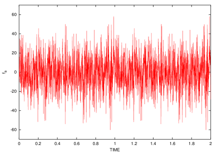
Figure 16: The quantity $f(t)$ obtained by summing over $1000$ oscillators with initial conditions drawn from a Gaussian distribution.

8.3.4 Markovian regime

We shall now study the form that the dynamical equations derived exhibit in the absence of memory effects. This occurs when the memory kernels are sharply peaked at $\tau=0$, the remainder terms in the memory integrals change slowly enough in the relevant range, and the kernels enclose a finite non-zero algebraic area. Under these conditions, one can replace the kernels by Dirac deltas and no memory effects occur.

Doing this with the memory kernel (8.27), we write

$${\cal K}_{{\rm a}{\rm b}}(\tau)=2\gamma_{{\rm a}{\rm b}}\delta(\tau)\;,$$ (8.31)

where the $\gamma_{{\rm a}{\rm b}}$ are damping coefficients related with the strength and characteristics of the coupling (see below). Then, on using $\int_{0}^{\infty}\!{\rm d}\tau\,\delta(\tau)h(\tau)=h(0)/2$, equation (8.26) reduces to

$${\framebox{$\displaystyle{\frac{{\rm d}A}{{\rm d}t}=\big{\{}A,{\cal H}\big{\}}+\sum_{{\rm a}}\big{\{}A,W_{{\rm a}}\big{\}}\bigg{[}f_{{\rm a}}(t)+\sum_{{\rm b}}\gamma_{{\rm a}{\rm b}}\frac{{\rm d}W_{{\rm b}}}{{\rm d}t}\bigg{]}\;,}$}}$$ (8.32)

with

$$\left\langle f_{{\rm a}}(t)\right\rangle=0\;,\qquad\left\langle f_{{\rm a}}(t)f_{{\rm b}}(t^{\prime})\right\rangle=2\gamma_{{\rm a}{\rm b}}k_{{\rm B}}T\,\delta(t-t^{\prime})\;.$$ (8.33)

Inspecting Eq. (8.31), one sees that the damping coefficients can be obtained from the area enclosed by the memory kernels or, alternatively, by inserting the definition of the kernel (8.28) into the corresponding integral and then using $\int_{0}^{\infty}\!{\rm d}\tau\,\cos(\omega\tau)=\pi\delta(\omega)$:

$$\gamma_{{\rm a}{\rm b}}=\int_{0}^{\infty}\!\!{\rm d}\tau\,{\cal K}_{{\rm a}{\rm b}}(\tau)\;,\qquad\gamma_{{\rm a}{\rm b}}=\pi\varepsilon^{2}\sum_{\alpha}\frac{c_{\alpha}^{{\rm a}}c_{\alpha}^{{\rm b}}}{\omega_{\alpha}^{2}}\delta(\omega_{\alpha})\;.$$ (8.34)

The area $\int_{0}^{\infty}\!\!{\rm d}\tau\,{\cal K}_{{\rm a}{\rm b}}(\tau)$ must be: (i) finite and (ii) different from zero, for the Markovian approximation to work. The second expression gives the damping coefficients in terms of the distribution of normal modes and system-environment coupling constants, and could be useful in cases where it could be difficult to find the kernels exactly.

8.4 Examples: Brownian particles and spins

In order to particularize the general expressions to definite situations, we only need to specify the structure of the coupling terms $F_{{\rm a}}$.

Brownian particle.

For instance, let us set $F_{\alpha}(p,q)=-c_{\alpha}q$ (bilinear coupling), and write down Eq. (8.24) for $A=q$ and $A=p$ with help from $\big{\{}p,B\big{\}}=-\partial B/\partial q$ and $\big{\{}q,B\big{\}}=\partial B/\partial p$. Then one gets ${\rm d}q/{\rm d}t=\partial{\cal H}/\partial p$ plus Eq. (8.3), which is the celebrated generalized Langevin equation for a “Brownian” particle. The fluctuating force is explicitly given by $f(t)=\sum_{\alpha}c_{\alpha}f_{\alpha}(t)$ and the memory kernel by ${\cal K}(\tau)=\sum_{\alpha}c_{\alpha}^{2}{\cal K}_{\alpha}(\tau)$. Naturally, in the Markovian limit ${\cal K}(\tau)=2m\gamma\delta(\tau)$ we have

$$\frac{{\rm d}q}{{\rm d}t}=\frac{\partial{\cal H}}{\partial p}\;,\qquad\frac{{\rm d}p}{{\rm d}t}=-\frac{\partial{\cal H}}{\partial q}+f(t)-\gamma\frac{{\rm d}q}{{\rm d}t}\;,$$ (8.35)

whose relaxation term comprises minus the velocity $-({\rm d}q/{\rm d}t)$ of the particle.

In general, when $\big{\{}A,F_{{\rm a}}\big{\}}$ in Eq. (8.32) is not constant, the fluctuating terms $f_{{\rm a}}(t)$ enter multiplying the system variables (multiplicative fluctuations). In this example, owing to the fact that $\big{\{}q,-c_{\alpha}q\big{\}}=0$ and $\big{\{}p,-c_{\alpha}q\big{\}}=c_{\alpha}$, the fluctuations are additive.

Spin-dynamics.

Let us now particularize the above results to the dynamics of a classical spin. To do so, we merely put $A=s_{i}$, $i=x,y,z$, in Eq. (8.24), and then use Eq. (8.14) to calculate the Poisson brackets required. Using also ${\rm d}W_{{\rm b}}/{\rm d}t=(\partial W_{{\rm b}}/\partial\vec{s})\cdot({\rm d}\vec{s}/{\rm d}t)$, we have

$$\frac{{\rm d}s_{i}}{{\rm d}t}=-\bigg{(}\vec{s}\wedge\frac{\partial{\cal H}}{\partial\vec{s}}\bigg{)}_{i}-\sum_{{\rm a}}\bigg{(}\vec{s}\wedge\frac{\partial W_{{\rm a}}}{\partial\vec{s}}\bigg{)}_{i}\bigg{[}f_{{\rm a}}(t)+\sum_{{\rm b}}\gamma_{{\rm a}{\rm b}}\frac{\partial W_{{\rm b}}}{\partial\vec{s}}\cdot\frac{{\rm d}\vec{s}}{{\rm d}t}\bigg{]}\;,$$

On gathering these results for $i=x,y,z$ in vectorial form and recalling the definition of the effective field $\vec{B}=-\partial{\cal H}/\partial\vec{s}$, we arrive at

$$\frac{{\rm d}\vec{s}}{{\rm d}t}=\vec{s}\wedge\vec{B}-\vec{s}\wedge\Bigg{(}\sum_{{\rm a}}f_{{\rm a}}(t)\frac{\partial W_{{\rm a}}}{\partial\vec{s}}+\bigg{[}\sum_{{\rm a}{\rm b}}\gamma_{{\rm a}{\rm b}}\frac{\partial W_{{\rm a}}}{\partial\vec{s}}\frac{\partial W_{{\rm b}}}{\partial\vec{s}}\bigg{]}\cdot\frac{{\rm d}\vec{s}}{{\rm d}t}\Bigg{)}\;.$$

Then, defining the fluctuating magnetic field

$$\vec{\xi}(t)=-\sum_{{\rm a}}f_{{\rm a}}(t)\frac{\partial W_{{\rm a}}}{\partial\vec{s}}\;,$$ (8.36)

and the second-rank tensor $\hat{\Lambda}$ with elements

$$\Lambda_{ij}=\sum_{{\rm a},{\rm b}}\gamma_{{\rm a}{\rm b}}\frac{\partial W_{{\rm a}}}{\partial s_{i}}\frac{\partial W_{{\rm b}}}{\partial s_{j}}\;,$$ (8.37)

we finally obtain the Langevin equation for the spin

$${\framebox{$\displaystyle{\frac{{\rm d}\vec{s}}{{\rm d}t}=\vec{s}\wedge\left[\vec{B}+\vec{\xi}(t)\right]-\vec{s}\wedge\hat{\Lambda}\frac{{\rm d}\vec{s}}{{\rm d}t}\;.}$}}$$ (8.38)

Equation (8.38) contains ${\rm d}\vec{s}/{\rm d}t$ on its right-hand side, so it will be referred to as a Gilbert-type equation. For $\varepsilon\ll 1$, on replacing perturbatively that derivative by its conservative part, ${\rm d}\vec{s}/{\rm d}t\simeq\vec{s}\wedge\vec{B}$, one gets the weak-coupling Landau–Lifshitz-type equation

$${\framebox{$\displaystyle{\frac{{\rm d}\vec{s}}{{\rm d}t}=\vec{s}\wedge\left[\vec{B}+\vec{\xi}(t)\right]-\vec{s}\wedge\hat{\Lambda}\left(\vec{s}\wedge\vec{B}\right)\;.}$}}$$ (8.39)

which describes weakly damped precession. From the statistical properties (8.33) of the fluctuating sources $f_{{\rm a}}(t)$, one gets

$$\left\langle\xi_{i}(t)\right\rangle=0\;,\quad\left\langle\xi_{i}(t)\xi_{j}(t^{\prime})\right\rangle=2\Lambda_{ij}k_{{\rm B}}T\delta(t-t^{\prime})\;,$$ (8.40)

which relates the structure of the correlations of the fluctuating field and the relaxation tensor.

For a general form of the spin-environment interaction, due to the occurrence of the tensor $\hat{\Lambda}$ the structure of the relaxation terms in the above equations deviates from the forms proposed by Gilbert and Landau and Lifshitz. However, if the spin-environment interaction yields uncorrelated and isotropic fluctuations ($\Lambda_{ij}=\lambda\delta_{ij}$), one finds that: (i) the statistical properties (8.40) reduce to those in (8.2) and (ii) the Langevin equation (8.39) reduces to the stochastic Landau–Lifshitz equation (8.2).

We remark in closing that the occurrence of the vector product $\vec{s}\wedge\vec{\xi}$ in the dynamical equations entails that the fluctuating terms enter in a multiplicative way. In the spin-dynamics case, in analogy with the results obtained for mechanical rigid rotators, the multiplicative character of the fluctuations is an inevitable consequence of the Poisson bracket relations for angular-momentum-type dynamical variables $\big{\{}s_{i},s_{j}\big{\}}=\sum_{k}\epsilon_{ijk}s_{k}$, which, even for $F_{{\rm a}}$ linear in $\vec{s}$, lead to non-constant $\big{\{}A,F_{{\rm a}}\big{\}}$ in Eq. (8.24). In our derivation this can straightly be traced back by virtue of the Hamiltonian formalism employed.

8.5 Discussion

We have seen that starting from a Hamiltonian description of a classical system interacting with the surrounding medium, one can derive generalized Langevin equations, which, in the Markovian approach, reduce to known phenomenological Langevin equations.

Note however that the presented derivation of the equations is formal in the sense that one must still investigate specific realizations of the system-plus-environment whole system, and then prove that the assumptions employed (mainly that of Markovian behavior) are at least approximately met. Let us give an example for a particle coupled to the elastic waves (phonons) of the substrate where it moves. The interaction would be proportional to the deformation tensor ${\cal H}_{\rm SE}\propto\partial u/\partial x$ in one dimension. Expanding the displacement field in normal modes $u(x)=\sum_{k}u_{k}\exp(\mathrm{i}kx)$, where the $u_{k}$ are the coordinates of the environment variables (our $Q_{\alpha}$), we have ${\cal H}_{\rm SE}\propto\sum_{k}\mathrm{i}k\exp(\mathrm{i}kx)u_{k}$, so that $c_{k}\propto\mathrm{i}k\exp(\mathrm{i}kx)$. If we had allowed complex $c_{\alpha}$, the products $c_{\alpha}^{2}$ would had been replaced by $|c_{\alpha}|^{2}$. Well, the corresponding memory kernel [Eq. (8.28)], then gives

$${\cal K}(\tau)=\varepsilon^{2}\sum_{\alpha}\frac{|c_{\alpha}|^{2}}{\omega_{\alpha}^{2}}\cos(\omega_{\alpha}\tau)\stackrel{{\scriptstyle\omega_{k}=ck}}{{\to}}\int_{0}^{k_{\rm D}}{\rm d}k\frac{{{}\not}k^{2}}{c^{2}{{}\not}k^{2}}\cos(ck\tau)\propto\frac{\sin(\omega_{\rm D}\tau)}{\tau}\;.$$

But, $\sin(\Omega\tau)/\tau$ plays the role of a Dirac delta for any process with time-scales much larger than $1/\Omega$. Thus, taking the Markovian limit is well justified in this case.

On the other hand, we have considered the classical regime of the environment and the system. A classical description of the environment is adequate, for example, for the coupling to low-frequency ($\hbar\omega_{\alpha}/k_{{\rm B}}T\ll 1$) normal modes. Nevertheless, the fully Hamiltonian formalism used, allows to guess the structure of the equations in the quantum case (just replacing Poisson brackets by commutators).

APPENDICES

Dynamical equations for the averages: macroscopic equation

From the master equation one can derive the dynamical equations for the averages of a Markov stochastic process. We shall write down the corresponding derivations directly in the multivariate case.

Let us first write the equation for the time evolution of an arbitrary function $\left\langle f({\bf{y}})\right\rangle$. First, one has

$$\frac{d{}}{d{t}}\left\langle{f({\bf{y}})}\right\rangle=\frac{d{}}{d{t}}{\displaystyle\int}\!{\rm d}{{\bf{y}}}\,f({\bf{y}})P({\bf{y}},t)={\displaystyle\int}\!{\rm d}{{\bf{y}}}\,f({\bf{y}})\frac{\partial{P({\bf{y}},t)}}{\partial{t}}\;.$$

Then, by using the master equation to express $\partial{P}/\partial{t}$, one has

$$\frac{d{}}{d{t}}\left\langle{f({\bf{y}})}\right\rangle = \underbrace{{\displaystyle\int}\!{\rm d}{{\bf{y}}}\,f({\bf{y}}){\displaystyle\int}\!{\rm d}{{\bf{y}}^{\prime}}\,W({\bf{y}}|{\bf{y}}^{\prime})P({\bf{y}}^{\prime},t)}_{{\bf{y}}^{\prime}\leftrightarrow{\bf{y}}}-{\displaystyle\int}\!{\rm d}{{\bf{y}}}\,f({\bf{y}}){\displaystyle\int}\!{\rm d}{{\bf{y}}^{\prime}}\,W({\bf{y}}^{\prime}|{\bf{y}})P({\bf{y}},t)$$ (.41)

$$= {\displaystyle\int}\!{\rm d}{{\bf{y}}^{\prime}}\,f({\bf{y}}^{\prime}){\displaystyle\int}\!{\rm d}{{\bf{y}}}\,W({\bf{y}}^{\prime}|{\bf{y}})P({\bf{y}},t)-{\displaystyle\int}\!{\rm d}{{\bf{y}}}\,f({\bf{y}}){\displaystyle\int}\!{\rm d}{{\bf{y}}^{\prime}}\,W({\bf{y}}^{\prime}|{\bf{y}})P({\bf{y}},t)$$

$$= {\displaystyle\int}\!{\rm d}{{\bf{y}}}\,P({\bf{y}},t){\displaystyle\int}\!{\rm d}{{\bf{y}}^{\prime}}\,[f({\bf{y^{\prime}}})-f({\bf{y}})]W({\bf{y}}^{\prime}|{\bf{y}})\;.$$

On applying now this equation to $f({\bf{y}})=y_{i}$, and defining [cf. Eq. (4.2)]

$$a_{i}^{(1)}({\bf{y}},t)={\displaystyle\int}\!{\rm d}{{\bf{y}}^{\prime}}\,(y_{i}^{\prime}-y_{i})W({\bf{y}}^{\prime}|{\bf{y}})\;,$$ (.42)

the last line in Eq. (.41) is the average of $a_{i}^{(1)}({\bf{y}},t)$, so we can finally write

$${\framebox{$\displaystyle{\frac{d{}}{d{t}}\left\langle{y_{i}}\right\rangle=\big{\langle}{a_{i}^{(1)}({\bf{y}},t)}\big{\rangle}\qquad(i=1,2,\ldots)\;.}$}}$$ (.43)

This is an exact consequence of the master equation and therefore holds for any Markov process.

Note that when $a_{i}^{(1)}$ is linear function of ${\bf{y}}$ one has $\big{\langle}{a_{i}^{(1)}({\bf{y}},t)}\big{\rangle}=a_{i}^{(1)}(\left\langle{{\bf{y}}}\right\rangle,t)$, whence

$$\frac{d{}}{d{t}}\left\langle{y_{i}}\right\rangle=a_{i}^{(1)}(\left\langle{{\bf{y}}}\right\rangle,t)\;,$$

which is a system of ordinary differential equations for $\left\langle{{\bf{y}}}\right\rangle$ and can be identified with the macroscopic equation of the system. For instance in the decay problem (4.9), since $W_{n^{\prime},n}$ is non-zero for $n^{\prime}=n-1$, we have

$$a^{(1)}(n,t)=\sum_{n^{\prime}}(n^{\prime}-n)\underbrace{W_{n^{\prime},n}}_{\gamma n\delta_{n^{\prime},n-1}}=[({{}\not}n-1)-{{}\not}n]\,\gamma n=-\gamma n\;.$$

Therefore, from the general result (.43) we have ${\rm d}\left\langle n\right\rangle/{\rm d}t=\langle a^{(1)}(n,t)\rangle=-\left\langle\gamma n\right\rangle$, in agreement with Eq. (4.10).

On the other hand, when $a_{i}^{(1)}$ is a non-linear function of ${\bf{y}}$, Eq. (.43) is not a differential equation for $\left\langle{y_{i}}\right\rangle$. Then Eq. (.43) is not a closed equation for $\left\langle{y_{i}}\right\rangle$ but higher-order moments enter as well. Thus, the evolution of $\left\langle{y_{i}}\right\rangle$ in the course of time is not determined by $\left\langle{y_{i}}\right\rangle$ itself, but is also influenced by the fluctuations around this average. To get equations for higher-order moments we proceed analogously. For instance, for $\left\langle{y_{i}(t)y_{j}(t)}\right\rangle$, we can use Eq. (.41) with $f({\bf{y}})=y_{i}y_{j}$. Writting $(y_{i}^{\prime}y_{j}^{\prime}-y_{i}y_{j})=(y_{i}^{\prime}-y_{i})(y_{j}^{\prime}-y_{j})+y_{i}(y_{j}^{\prime}-y_{j})+y_{j}(y_{i}^{\prime}-y_{i})$, and defining, analogously to Eqs. (4.2) and (.42),

$$a_{ij}^{(2)}({\bf{y}},t)={\displaystyle\int}\!{\rm d}{{\bf{y}}^{\prime}}\,(y_{i}^{\prime}-y_{i})(y_{j}^{\prime}-y_{j})W({\bf{y}}^{\prime}|{\bf{y}})\;.$$ (.44)

we finally have

$${\framebox{$\displaystyle{\frac{d{}}{d{t}}\left\langle{y_{i}y_{j}}\right\rangle=\big{\langle}{a_{ij}^{(2)}({\bf{y}},t)}\big{\rangle}+\big{\langle}{y_{i}a_{j}^{(1)}({\bf{y}},t)}\big{\rangle}+\big{\langle}{y_{j}a_{i}^{(1)}({\bf{y}},t)}\big{\rangle}\;.}$}}$$ (.45)

which is also an exact consequence of the master equation. However, if $a_{ij}^{(2)}$ is a non-linear function of ${\bf{y}}$, the equation involves even higher order moments $\left\langle y_{i}y_{j}y_{k}\right\rangle$, so what we have is an infinite hierarchy of coupled equations for the moments.

The Langevin process $\xi(t)$ as the derivative of the Wiener–Lévy process

Let us formally write ${\rm d}W/{\rm d}t=\xi(t)$, and see which are the properties of the $W(t)$ so defined. On integrating over an interval $\tau$, we have

$$w(\tau)\equiv\Delta W(\tau)\equiv W(t+\tau)-W(t)=\int_{t}^{t+\tau}\!\!\xi(s)ds\;.$$ (.47)

Let us show that this $w(\tau)$ is indeed a Wiener–Lévy process. Firstly, $w(\tau)$ is Gaussian because $\xi(t)$ is so. Furthermore, on using the statistical properties (5.1) one gets ($\tau,\tau_{1},\tau_{2}\geq 0$)

$$w(0)=0\;,\qquad\left\langle{w(\tau)}\right\rangle=0\;,\qquad\left\langle{w(\tau_{1})w(\tau_{2})}\right\rangle=2D\min(\tau_{1},\tau_{2})\;.$$ (.48)

Proof: $w(0)=0$ follows immediately from the definition (.47), while for the average $\left\langle{w(\tau)}\right\rangle$, one gets $\left\langle{w(\tau)}\right\rangle=\int_{t}^{t+\tau}\!\!\,\underbrace{\left\langle{\xi(s)}\right\rangle}_{0}ds=0$. On the other hand, for $\left\langle{w(\tau_{1})w(\tau_{2})}\right\rangle$, one finds

$$\left\langle{w(\tau_{1})w(\tau_{2})}\right\rangle = \int_{t}^{t+\tau_{1}}\int_{t}^{t+\tau_{2}}\,\overbrace{\left\langle{\xi(s)\xi(s^{\prime})}\right\rangle}^{2D\delta(s-s^{\prime})}ds^{\prime}ds$$

$$= 2D\int_{t}^{t+\min(\tau_{1},\tau_{2})}\,\overbrace{\int_{t}^{t+\max(\tau_{1},\tau_{2})}\,\,\delta(s-s^{\prime})ds^{\prime}}^{1}ds$$

$$= 2D\min(\tau_{1},\tau_{2})\;,$$

where we have sorted the integrals to ensure that, when using the Dirac delta to take one of them, the location of the “maximum” of the delta is inside the corresponding integration interval, and the result is therefore unity.

Now on comparing these results with those for the increment of the Wiener–Lévy process, whose average is zero since that of the Wiener–Lévy process is zero and the second moment is given by Eqs. (3.12), one realises that the process defined by Eq. (.47) coincides with the increment of a Wiener–Lévy process.

Proof of the convergence of the Heun scheme

We shall check that the Heun scheme correctly generates the Kramers–Moyal coefficients, by carrying out the Taylor expansion of Eq. (7.1.2), accounting for Eq. (7.5). Concerning the terms involving $A_{i}$, one has

$$\tfrac{1}{2}\left\{{A_{i}(\tilde{{\bf{y}}},t+\Delta t)+A_{i}[{\bf{y}}(t),t]}\right\}\Delta t$$

$$=\tfrac{1}{2}\bigg{\{}{A_{i}[{\bf{y}}(t),t]+\frac{\partial{A_{i}}}{\partial{t}}\Delta t+\sum_{j}\frac{\partial{A_{i}}}{\partial{y_{j}}}\overbrace{[\tilde{y}_{j}-y_{j}(t)]}^{\hbox to0.0pt{$\displaystyle\qquad{\scriptstyle{A_{j}\Delta t+\sum_{k}B_{jk}\Delta W_{k}}}$\hss}}+\cdots+A_{i}[{\bf{y}}(t),t]}\bigg{\}}\Delta t$$

$$=A_{i}[{\bf{y}}(t),t]\Delta t+{\cal O}[(\Delta t)^{3/2}]\;,$$

whereas, the terms involving $B_{ik}$ can be expanded as

$$\tfrac{1}{2}\left\{{B_{ik}(\tilde{{\bf{y}}},t+\Delta t)+B_{ik}[{\bf{y}}(t),t]}\right\}\Delta W_{k}$$

$$= \tfrac{1}{2}\bigg{\{}{B_{ik}[{\bf{y}}(t),t]+\frac{\partial{B_{ik}}}{\partial{t}}\Delta t+\sum_{k}\frac{\partial{B_{ik}}}{\partial{y_{j}}}\overbrace{[\tilde{y}_{j}-y_{j}(t)]}^{\hbox to0.0pt{$\displaystyle\qquad{\scriptstyle{A_{j}\Delta t+\sum_{\ell}B_{j\ell}\Delta W_{\ell}}}$\hss}}+\cdots+B_{ik}[{\bf{y}}(t),t]}\bigg{\}}\Delta W_{k}$$

$$= B_{ik}[{\bf{y}}(t),t]\Delta W_{k}+\sum_{k}\frac{\partial{B_{ik}}}{\partial{y_{j}}}[{\bf{y}}(t),t]\sum_{\ell}B_{j\ell}[{\bf{y}}(t),t]\Delta W_{\ell}\Delta W_{k}+{\cal O}[(\Delta t)^{3/2}]\;.$$

In this case we have retained in $\tilde{y}_{j}-y_{j}(t)$ terms up to order $(\Delta t)^{1/2}$, which in the corresponding expansion of $A_{i}$ are omitted since they yield terms of order $(\Delta t)^{3/2}$. Finally, on inserting these expansions in Eq. (7.1.2), on gets

$$y_{i}(t+\Delta t)\simeq y_{i}(t)+A_{i}[{\bf{y}}(t),t]\Delta t+\sum_{k}B_{ik}[{\bf{y}}(t),t]\Delta W_{k}$$

$${}+\frac{1}{2}\sum_{k\ell}\bigg{\{}{\sum_{j}B_{j\ell}[{\bf{y}}(t),t]\frac{\partial{B_{ik}}}{\partial{y_{j}}}[{\bf{y}}(t),t]}\bigg{\}}\Delta W_{k}\Delta W_{\ell}\;,$$ (.49)

which corresponds to Eq. (2.8) of Ramírez-Piscina, Sancho and Hernández-Machado. Finally, to obtain the Kramers–Moyal coefficients, we have to average Eq. (Proof of the convergence of the Heun scheme) for fixed initial values ${\bf{y}}(t)$ (conditional average). To do so, one can use $\left\langle{\Delta W_{k}}\right\rangle=0$ and $\left\langle{\Delta W_{k}\Delta W_{\ell}}\right\rangle=(2D\Delta t)\delta_{k\ell}$, to get

$$\bigg{\langle}{\sum_{k}B_{ik}\Delta W_{k}}\bigg{\rangle} = 0\;,$$

$$\bigg{\langle}{\frac{1}{2}\sum_{jk\ell}B_{j\ell}\frac{\partial{B_{ik}}}{\partial{y_{j}}}\Delta W_{k}\Delta W_{\ell}}\bigg{\rangle} = D\bigg{(}{\sum_{jk}B_{jk}\frac{\partial{B_{ik}}}{\partial{y_{j}}}}\bigg{)}\Delta t\;,$$

$$\bigg{\langle}{\sum_{k}B_{ik}\Delta W_{k}\sum_{\ell}B_{j\ell}\Delta W_{\ell}}\bigg{\rangle} = 2D\bigg{(}{\sum_{k}B_{ik}B_{jk}}\bigg{)}\Delta t\;.$$

Therefore, from Eq. (Proof of the convergence of the Heun scheme) one obtains

$$\left\langle{y_{i}(t+\Delta t)-y_{i}(t)}\right\rangle=\bigg{(}{A_{i}+D\sum_{jk}B_{jk}\frac{\partial{B_{ik}}}{\partial{y_{j}}}}\bigg{)}\Delta t+{\cal O}[(\Delta t)^{3/2}]$$

$$\left\langle{\left[{y_{i}(t+\Delta t)-y_{i}(t)}\right]\left[{y_{j}(t+\Delta t)-y_{j}(t)}\right]}\right\rangle=2D\bigg{(}{\sum_{k}B_{ik}B_{jk}}\bigg{)}\Delta t+{\cal O}[(\Delta t)^{3/2}]\;,$$

which lead to the Kramers–Moyal coefficients (5.3.1) via Eq. (4.21). Q.E.D.

Proof of the Box–Muller algorithm.

We can verify that the transformation (7.6) leads to a pair of independent Gaussian random numbers as an exercise of transformation of variables as introduced in Sec. 2.4:

$$P_{W_{1},W_{2}}(w_{1},w_{2}) = {\displaystyle\int_{0}^{1}}\!{\rm d}{r_{1}}\,\!{\displaystyle\int_{0}^{1}}\!{\rm d}{r_{2}}\,\delta[w_{1}-\sqrt{-2\ln(r_{1})}\cos(2\pi r_{2})]$$

$$\hskip 55.00008pt{}\times\delta[w_{2}-\sqrt{-2\ln(r_{1})}\sin(2\pi r_{2})]\overbrace{P_{R_{1},R_{2}}(r_{1},r_{2})}^{1~{}\text{by~{}hypothesis}}\;.$$

Let us now introduce the substitution

$$u_{1}(r_{1},r_{2})=\sqrt{-2\ln(r_{1})}\cos(2\pi r_{2})\;,\quad u_{2}(r_{1},r_{2})=\sqrt{-2\ln(r_{1})}\sin(2\pi r_{2})\;,$$

the Jacobi matrix of which reads

$$\left(\begin{array}[]{cc}\frac{\partial{u_{1}}}{\partial{r_{1}}}&\frac{\partial{u_{1}}}{\partial{r_{2}}}\\[8.61108pt] \frac{\partial{u_{2}}}{\partial{r_{1}}}&\frac{\partial{u_{2}}}{\partial{r_{2}}}\end{array}\right)=\left(\begin{array}[]{cc}-\frac{1}{r_{1}}\frac{1}{\sqrt{-2\ln(r_{1})}}\cos(2\pi r_{2})&-2\pi\sqrt{-2\ln(r_{1})}\sin(2\pi r_{2})\\ -\frac{1}{r_{1}}\frac{1}{\sqrt{-2\ln(r_{1})}}\sin(2\pi r_{2})&\quad 2\pi\sqrt{-2\ln(r_{1})}\cos(2\pi r_{2})\end{array}\right)$$

and the corresponding Jacobian (the determinant of this matrix) is given by $\partial{(u_{1},u_{2})}/\partial{(r_{1},r_{2})}=-{2\pi}/{r_{1}}$. Nevertheless, when changing the variables in the above integrals one needs the absolute value of the Jacobian of the inverse transformation, which is given by $|\partial{(r_{1},r_{2})}/\partial{(u_{1},u_{2})}|={r_{1}}/{2\pi}$. Besides, $r_{1}(u_{1},u_{2})$ can be obtained from the above transformation: $-2\ln(r_{1})=u_{1}^{2}+u_{2}^{2}$ $\Rightarrow$ $r_{1}=\exp[-\frac{1}{2}\left(u_{1}^{2}+u_{2}^{2}\right)]$. On using all these results the probability distribution of $(w_{1},w_{2})$ is finally given by

$$P_{W_{1},W_{2}}(w_{1},w_{2}) = {\displaystyle\int_{-\infty}^{\infty}}\!{\rm d}{u_{1}}\,{\displaystyle\int_{-\infty}^{\infty}}\!{\rm d}{u_{2}}\,\delta(w_{1}-u_{1})\delta(w_{2}-u_{2})\frac{1}{2\pi}\exp\left[{-\tfrac{1}{2}\left(u_{1}^{2}+u_{2}^{2}\right)}\right]$$

$$= \frac{1}{\sqrt{2\pi}}\exp\left({-\tfrac{1}{2}w_{1}^{2}}\right)\frac{1}{\sqrt{2\pi}}\exp\left({-\tfrac{1}{2}w_{2}^{2}}\right)\;.$$

This expression demonstrates that when $r_{1}$ and $r_{2}$ are independent random numbers uniformly distributed in the interval $(0,1)$, the random variables $w_{1}$ and $w_{2}$ given by the transformation (7.6) are indeed independent and Gaussian-distributed with zero mean and variance unity.

References

• [1] A. O. Caldeira and A. J. Leggett, Dissipation and quantum tunnelling, Ann. Phys. (NY) 149 (1983), 374–456, Physica A 121, 587 (1983).
• [2] C. W. Gardiner, Handbook of stochastic methods, 2nd ed., Springer, Berlin, 1990.
• [3] W. H. Press, S. A. Teukolsky, W. T. Vetterling, and B. P. Flannery, Numerical recipes, 2nd ed., Cambridge University Press, New York, 1992.
• [4] H. Risken, The Fokker–Planck equation, 2nd ed., Springer, Berlin, 1989.
• [5] N. G. van Kampen, Stochastic processes in physics and chemistry, 2nd ed., North-Holland, Amsterdam, 1992.
• [6] H. S. Wio, An introduction to stochastic processes and nonequilibrium statistical physics, World Scientific, Singapore, 1994, Series on advances in statistical mechanics – vol. 10.