Magnetic shielding properties of high-temperature superconducting tubes subjected to axial fields

1 abstract

We have experimentally studied the magnetic shielding properties of a cylindrical shell of BiPbSrCaCuO subjected to low frequency AC axial magnetic fields. The magnetic response has been investigated as a function of the dimensions of the tube, the magnitude of the applied field, and the frequency. These results are explained quantitatively by employing the method of E. H. Brandt (Brandt E H 1998 Phys. Rev. B 58 6506) with a $J_{c}(B$) law appropriate for a polycrystalline material. Specifically, we observe that the applied field can sweep into the central region either through the thickness of the shield or through the opening ends, the latter mechanism being suppressed for long tubes. For the first time, we systematically detail the spatial variation of the shielding factor (the ratio of the applied field over the internal magnetic field) along the axis of a high-temperature superconducting tube. The shielding factor is shown to be constant in a region around the centre of the tube, and to decrease as an exponential in the vicinity of the ends. This spatial dependence comes from the competition between two mechanisms of field penetration. The frequency dependence of the shielding factor is also discussed and shown to follow a power law arising from the finite creep exponent $n$.

2 Introduction

Electromagnetic shielding has two main purposes. The first one is to prevent an electronic device from radiating electromagnetic energy, in order to comply with radiation regulations, to protect neighbouring equipments from electromagnetic noise, or, in certain military applications, to reduce the electromagnetic signature of the device. The second purpose of shielding is to protect sensitive sensors from radiation emitted in their surroundings, in order to take advantage of their full capabilities.

As long as the frequency of the source field remains large, typically $f>1\leavevmode\nobreak\ \mathrm{kHz}$, conducting materials can be used to attenuate the field with the skin effect. For the lowest frequencies, however, conductors continue to act as good electric shields (and can be used to make a Faraday cage), but they fail to shield magnetic fields. The traditional approach to shield low frequency magnetic fields consists in using soft ferromagnetic materials with a high relative permeability, which divert the source field from the region to protect [1]. As the magnetic permeability decreases with increasing frequency, this approach is only practical for low frequencies (typically $f<1\leavevmode\nobreak\ \mathrm{kHz}$). If low temperatures are allowed by the application (77 K for cooling with liquid nitrogen), shielding systems based on high-temperature superconductors (HTS) compete with the traditional solutions [2]. Below their critical temperature, $T_{c}$, HTS are strongly diamagnetic and expel a magnetic flux from their bulk. They can be used to construct enclosures that act as very effective magnetic shields over a broad frequency range [2].

Several factors determine the quality of a HTS magnetic shield. First, a threshold induction, $B_{\mathrm{lim}}$, characterizes the maximum applied induction that can be strongly attenuated. In the case of a shield that is initially not magnetized and is subjected to an increasing applied field, the internal field remains close to zero until the applied induction rises above $B_{\mathrm{lim}}$. The field then penetrates the inner region of the shield and the induction increases with the applied field [3, 4, 5, 6, 7, 8]. A second important factor is the geometrical volume over which a shield of given size and shape can attenuate an external field below a given level. A third determining factor is the frequency response of the shield.

In this paper, we focus on the shielding properties of a ceramic tube in the parallel geometry, which means that the source field is applied parallel to the tube axis. This geometry is amenable to direct physical interpretation and numerical simulations, as currents flow along concentric circles perpendicular to the axis. Note that a HTS tube certainly outperforms a ferromagnetic shield in the parallel geometry [9]. For a ferromagnetic tube with an infinite length, the shield does not attenuate the external magnetic field since its longitudinal component must be continuous accross the air-ferromagnet interface. For finite lengths, the magnetic flux is caught in the material because of demagnetization effects but the shielding efficiency remains poor for long tubes.

A number of results can be found in the literature on HTS tubes in the parallel geometry. For HTS polycrystalline materials, $B_{\mathrm{lim}}$ was found to vary between $0.3\leavevmode\nobreak\ \mathrm{mT}$ for a tube with a superconducting wall of thickness $d=40\leavevmode\nobreak\ \mu\mathrm{m}$ [10, 11], and $15\leavevmode\nobreak\ \mathrm{mT}$ for $d=2.2\leavevmode\nobreak\ \mathrm{mm}$ [8] at $77\leavevmode\nobreak\ \mathrm{K}$. If lower temperatures are allowed than $77\leavevmode\nobreak\ \mathrm{K}$, higher $B_{\mathrm{lim}}$ values can be obtained with other compounds. As an example, MgB₂ tubes were reported to shield magnetic inductions up to $1\leavevmode\nobreak\ \mathrm{T}$ at $4.2\leavevmode\nobreak\ \mathrm{K}$ [12, 13]. Results on the variation of the field attenuation along the axis appear to be contradictory. An exponential dependence was measured for a YBCO tube [14] and for a BSCCO tube  [15]. Other measurements [7, 16] in similar conditions have shown instead a constant shielding factor in a region around the centre of YBCO and BSCCO tubes. As for the frequency response, the shielding factor is expected to be constant if flux creep effects are negligible, as is the case in Bean’s model [17, 18]. It is on the other hand expected to increase with frequency in the presence of flux creep, since the induced currents saturate to values that increase with frequency [19]. Experimental data have shown very diverse behaviours. In [15], the field attenuation due to a thick BSCCO film on a cylindrical silver substrate was found to be frequency independent. The same results were established for superconducting disks made from YBCO powder and subjected to perpendicular fields [20, 21]. Yet other studies on bulk BSCCO tubes [3, 22] measured a field attenuation that decreases with frequency, whereas the attenuation was shown to slowly increase with frequency for a YBCO superconducting tube [23].

The purpose of this paper is to provide a detailed study of the magnetic shielding properties of a polycrystalline HTS tube, with regard to the three determining factors: threshold induction, spatial variation of the field attenuation, and frequency response. The study is carried both experimentally and by means of numerical simulations, in order to shed light on the relation between the microscopic mechanisms of flux penetration and the macroscopic properties. For the numerical simulations, we have followed the method proposed by E. H. Brandt in [19], which can be carried easily with good precision on a personal computer. We focus on a HTS tube with one opening at each end and assume that the superconducting properties are uniform along the axis and isotropic.

The report is organized as follows. The sample and the experimental setup are described in section 3. In section 4, we discuss the constitutive laws that are appropriate for a polygrain HTS, set up the main equations and the numerical model. Section 5 is devoted to the shielding properties of superconducting tubes subjected to slowly time varying applied fields (called the DC mode). First, the evolution of the measured internal magnetic induction of a commercial sample versus the applied induction is presented. We then detail the field penetration into a HTS tube and study the field attenuation as a function of position along the tube axis. The frequency response of the shield is addressed in section 6, where it is shown that the variations with frequency can be explained by scaling laws provided heat dissipation can be neglected. Our main results are summarized in section 7, where we also draw conclusions of practical interest.

3 Experimental

Table 1: Physical characteristics of the sample: the material composition and the critical temperature come from [24]

Material	Bi1.8Pb0.26Sr2Ca2Cu3O10+x
Length	$\ell=8\leavevmode\nobreak\ \mathrm{cm}$
Inner radius	$a_{1}=6.5\leavevmode\nobreak\ \mathrm{mm}$
Outer radius	$a_{2}=8\leavevmode\nobreak\ \mathrm{mm}$
Wall thickness	$d=1.5\leavevmode\nobreak\ \mathrm{mm}$
Critical temperature	$T_{c}\cong 108\leavevmode\nobreak\ \mathrm{K}$

We measured the shielding properties of a commercial superconducting specimen (type CST-12/80 from CAN Superconductors), which was cooled at $T=77\leavevmode\nobreak\ \mathrm{K}$ under zero-field. The sample is a tube made by isostatic pressing of a polygrain ceramic. Its main characteristics are summarized in table 1.

The experimental setup is shown in figure 1. The sample is immersed in liquid nitrogen and placed inside a source coil generating an axial magnetic induction $\mathbf{B}_{a}=B_{a}\,\hat{z}$. The applied induction, $B_{a}$, can be generated in two different modes. In the first mode, called the DC mode, $B_{a}$ increases at a constant rate of $\dot{B}_{a}\cong 0.2\leavevmode\nobreak\ \mathrm{mT/s}$ with a brief stop (around 1 second) needed to measure the internal induction at each wanted value of $B_{a}$. The maximum applied induction in this mode is $30\leavevmode\nobreak\ \mathrm{mT}$. The induction in the inside of the shield, $B_{\mathrm{in}}$, is measured with a Hall probe placed in the centre of the tube; the probe is connected to a HP34420 nanovoltmetre. To reduce noise from outside sources, the setup is enclosed in a double mu-metal ferromagnetic shield. The field resolution is around $1\leavevmode\nobreak\ \mathrm{\mu T}$. In the second mode of operation, called the AC mode, the applied field is a low-frequency alternating field with no DC component. The frequency of the applied induction ranges between $43\leavevmode\nobreak\ \mathrm{Hz}$ and $403\leavevmode\nobreak\ \mathrm{Hz}$ and the amplitude of $B_{a}$ can reach $25\leavevmode\nobreak\ \mathrm{mT}$. The field inside the tube is measured by a pick-up coil, which can be moved along the $z-$axis and whose induced voltage is measured with an EGG7260 lock-in amplifier. In this mode, the setup can measure magnetic inductions as weak as $1\leavevmode\nobreak\ \mathrm{nT}$ at $103\leavevmode\nobreak\ \mathrm{Hz}$. As a result, care must be taken to reject common-mode electrical noise. In the present work, the capacitive coupling between the source and the pick-up coils was reduced by electrically connecting the superconducting tube to ground so as to realize an electrical shield.

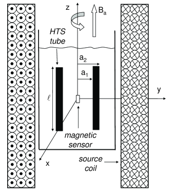
Figure 1: Experimental setup. The superconducting tube of length $\ell$ and wall tickness $d=a_{2}-a_{1}$ is placed inside a coil generating an axial induction of magnitude $B_{a}$. The applied field can have the form of a slow ramp, in which case the magnetic sensor is a Hall probe connected to a nanovoltmetre, or a that of a low-frequency alternating field, in which case the field inside the tube is measured by a pick-up coil connected to a lock-in amplifier. In all cases, the sample and the sensor are cooled with liquid nitrogen (T = 77 K) under zero-field condition.

4 Theory

4.1 Flux penetration in polycrystalline bulk ceramics

Bulk polycrystalline BiSrCaCuO ceramics consist of a stack of a large number of superconducting grains [25]. The penetration of a magnetic flux in such a material is inhomogeneous and strongly depends on the microstructure, as shielding currents can flow both in the grains and the intergranular matrix [26]. For a polygrain material that has been cooled in zero-field condition, the flux penetrates in roughly three different steps [27]. First, for the weakest applied fields, Meissner surface currents shield the volume and no flux enters the sample. When the local induction, $B$, exceeds $\mu_{0}\,H_{c1j}$, where $H_{c1j}$ is the lower critical field of the intergranular matrix, vortices start entering this region. The magnetic flux penetrates the grains at the higher induction $B\sim\mu_{0}H_{c1g}$ [28], where $H_{c1g}$ is the lower critical field of the grains themselves.

4.2 Model assumptions

In our model, we neglect surface barrier effects and set $H_{c1j}$ to zero. Therefore, flux starts threading the intergranular matrix as soon as the applied field is turned on. The penetration of individual grains depends on the intensity of the local magnetic field, which, because of demagnetization effects, varies as a function of the grain sizes and orientations. The penetration of each grain may thus take place over a range of applied fields: we expect an increasing number of grains to be penetrated as the external field is increased. Since we aim at studying the macroscopic properties of the superconducting tube and aim at deriving recommandations of practical interest, we will not seek to describe grains individually and thus neglect detailed effects of their diamagnetism. We will instead consider the induction $\mathbf{B}$ to be an average of the magnetic flux over many grains and assume the constitutive law $\mathbf{B}=\mu_{0}\,\mathbf{H}$. The resulting model describes the magnetic properties of an isotropic material which supports macroscopic shielding currents.

We will further assume the material to obey the conventional [19, 29] constitutive law

$$\mathbf{E}(J)=E_{c}\left({J\over J_{c}}\right)^{n}\>\frac{\mathbf{J}}{J},$$ (1)

where $J$ is the module of the vector current density $\mathbf{J}$. The exponent $n$ allows for flux creep and typically ranges from 10 to 40 for YBCO and BSCCO compounds at 77 K. The value for $n$ that is adequate for the sample of table 1 is to be determined from the frequency dependence of its shielding properties, see section 6.3. Note that one recovers Bean’s model, which neglects flux creep effects, by taking the limit $n\rightarrow\infty$. A final constitutive law comes from the polygrain nature of the material. The critical current density is assumed to decrease with the local induction as in Kim’s model [30]:

$$J_{c}(B)=\frac{J_{c0}}{1+B/B_{1}},$$ (2)

where $J_{c0}$ and $B_{1}$ are experimentally determined by fitting magnetization data, as discussed in section 5.2.

4.3 Model equations and numerical algorithm

A common difficulty in modelling the flux penetration in HTS materials arises from the fact that the direction of the shielding currents is usually not known a priori and, furthermore, may evolve over time as the flux front moves into the sample. This problem is greatly simplified for geometries in which the direction of the shielding currents is imposed by symmetry. Examples include long bars in a perpendicular applied field [29], in which case the currents flow along the bar, and axial symmetric specimens subjected to an axial field, for which the currents flow along concentric circles perpendicular to the symmetry axis. Numerous examples have been extensively studied by E. H. Brandt [31] for both geometries, by means of a numerical method based on the discretization of Biot-Savart integral equations. In this work, we follow Brandt’s method for modelling the flux penetration in a tube subjected to an axial field.

To set up the main equations, we closely follow [19]. As a reminder, the sample is a tube of internal radius $a_{1}$, external radius $a_{2}$, and length $\ell$ (see figure 1). We work with cylindrical coordinates, so that positions are denoted by $(r,\varphi,z)$. As the magnitude of the axial induction, $B_{a}$, is increased, the induced electric field and the resulting current density assume the form

$$\mathbf{J}=-J(r,z)\,\hat{\varphi},\quad\mathbf{E}=-E(r,z)\,\hat{\varphi},$$ (3)

where $\hat{\varphi}$ is the unit vector in the azimuthal direction. The magnetic induction is invariant under a rotation around the $z$-axis and has no $\varphi$-component. Thus,

$$\mathbf{B}(r,z)=B_{r}(r,z)\,\hat{r}+B_{z}(r,z)\,\hat{z}.$$ (4)

The fields $\mathbf{B}$, $\mathbf{E}$, and the current density, $\mathbf{J}$, satisfy Maxwell’s equations

$$\nabla\times\mathbf{E} = -\frac{\partial\mathbf{B}}{\partial t},$$ (5)

$$\nabla\times\mathbf{B} = \mu_{0}\,\mathbf{J},$$ (6)

where we have used the constitutive law $\mathbf{B}=\mu_{0}\mathbf{H}$.

In order to avoid an explicit and costly computation of the magnetic induction $\mathbf{B}(\mathbf{r},t)$ in the infinite region exterior to the tube, an equation of motion is first established for the macroscopic shielding current density $\mathbf{J}(\mathbf{r},t)$, since its support is limited to the volume of the superconductor. The magnetic field is then obtained where required by integrating the Biot-Savart law. After having eliminated $\mathbf{B}$ and integrated over $\varphi$, this procedure leads to the integral equation [19]

$$E(\mathbf{r})=-\mu_{0}\int^{a_{2}}_{a_{1}}\int^{\ell/2}_{0}Q(\mathbf{r},\mathbf{r^{\prime}})\dot{J}(\mathbf{r^{\prime}})\mathrm{d}r^{\prime}\mathrm{d}z^{\prime}+\frac{r}{2}\dot{B}_{a},$$ (7)

where $\mathbf{r}$ and $\mathbf{r^{\prime}}$ are shorthands for $(r,z)$ and $(r^{\prime},z^{\prime})$, while $Q(\mathbf{r},\mathbf{r^{\prime}})$ is a kernel which only depends on the sample geometry. In the present case, $Q$ assumes the form

$$Q(\mathbf{r},\mathbf{r^{\prime}})=f(r,r^{\prime},z-z^{\prime})+f(r,r^{\prime},z+z^{\prime}),$$ (8)

where

$$f(r,r^{\prime},\eta)=\int^{\pi}_{0}\frac{r^{\prime}\cos\varphi}{2\pi\sqrt{\eta^{2}+r^{2}+r^{\prime 2}-2rr^{\prime}\cos\varphi}}\>\mathrm{d}\varphi,$$ (9)

is to be evaluated numerically as suggested in [19]. By contrast to [19], the kernel is integrated in the radial direction from $r^{{}^{\prime}}=a_{1}$ to $r^{{}^{\prime}}=a_{2}$, as dictated by the tubular geometry of the sample.

The equation of motion for $\mathbf{J}$ is obtained in three steps. First, the electric field is eliminated from (7) by using the constitutive law (1). Second, the equation is discretized on a two-dimensional grid with spatial steps $\Delta r$ and $\Delta z$. Third, the resulting matrix equation is inverted, yielding the relation

$$\dot{J}_{i}(t)=\frac{1}{\mu_{0}\Delta r\Delta z}\sum_{j}Q_{ij}^{-1}\left\{\frac{r_{j}}{2}\dot{B}_{a}-E\left[J_{j}(t)\right]\right\}.$$ (10)

Here, $J_{i}$ and $Q_{ij}$ are shorthands for $J(\mathbf{r}_{i})$ and $Q(\mathbf{r}_{i},\mathbf{r}_{j})$. Actually, the two-dimensional space matrix is transformed into a one-dimensional vector. Imposing the initial condition

$$J_{i}(t=0)=0\quad\forall i,$$ (11)

the current density can be numerically integrated over time by updating the relation

$$J_{i}(t+\Delta t)\cong J_{i}(t)+\dot{J}_{i}(t)\,\Delta t,$$ (12)

where $\dot{J}_{i}$ is evaluated as in (10) and $\Delta t$ is chosen suitably small. An adaptative time step procedure described in [19] makes the algorithm converge towards a solution that reproduces the experimental data fairly well, see sections 5 and 6. Note that for those geometries that have one dimension much larger than the others, as is the case for a long tube with a thin wall, one can improve the convergence while preserving the precision by working with rectangular cells with the refinement described in [32].

According to the two different modes of operation of the external source that were introduced in section 3, we have run the algorithm with $B_{a}(t)$ either in the form of a ramp, $B_{a}(t)=\dot{B}_{a}\,t$, or as a sinusoidal source of frequency $f$, $B_{a}(t)=B_{o}\,\mathrm{sin}(2\pi ft)$. The shielding properties of the sample are evaluated in both cases by probing the magnetic flux density at points located along the $z$-axis of the tube. By symmetry, this field is directed along $\hat{z}$, and we define $B_{z\mathrm{in}}(z)$ as

$$\mathbf{B}(r=0,z)=B_{z\mathrm{in}}(z)\,\hat{z}.$$ (13)

For the DC mode, with $B_{a}=\dot{B}_{a}\,t$, we define the DC shielding factor as

$$DCSF(z)=\frac{B_{a}}{B_{z\mathrm{in}}(z)}.$$ (14)

However, in the AC mode, with $B_{a}(t)=B_{o}\,\mathrm{sin}(2\pi ft)$ , one must pay attention to the non-linearity of the magnetic response of the sample. The induction $B_{z\mathrm{in}}$ contains several harmonics, all odd in the absence of a DC component [33]. We are led to define the AC shielding factor as

$$ACSF(z)=\frac{B_{a,RMS}}{B_{z\mathrm{in},RMS}(z)},$$ (15)

where $B_{a,RMS}=B_{o}/\sqrt{2}$ is the RMS value of the applied magnetic induction and $B_{z\mathrm{in},RMS}(z)$ is the RMS value of the fundamental component of $B_{z\mathrm{in}}$, which can be directly measured by the lock-in amplifier.

The algorithm presented in this section allows us the determine $DCSF$ up to $10^{7}$ in the DC mode and $ACSF$ up to $10^{4}$ in the AC mode.

5 Magnetic shielding in the DC mode

5.1 Experimental results

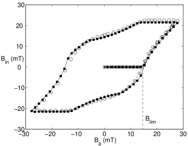
Figure 2: Evolution of the internal magnetic induction at the centre of the tube, $B_{z\mathrm{in}}(z=0)$, as a function of the applied induction. The sample (table 1) is cooled in zero-field conditions down to $T=77\leavevmode\nobreak\ \mathrm{K}$. The open circles represent the experimental data and the filled squares represent the simulation, as discussed in subsection 5.2.

Figure 2, open circles, shows the evolution of the magnetic induction measured at the centre of the tube, $B_{\mathrm{in}}\equiv B_{z\mathrm{in}}(z=0)$, as a function of the applied magnetic induction. Here, the external source was operated in the DC mode. The sample described in section 3 was cooled down to $77\leavevmode\nobreak\ \mathrm{K}$ in zero-field conditions. Then, we applied an increasing magnetic induction and reached $B_{a}=28\leavevmode\nobreak\ \mathrm{mT}$. Upon decreasing the applied induction to $B_{a}=-28\leavevmode\nobreak\ \mathrm{mT}$ and increasing it again up to $B_{a}=28\leavevmode\nobreak\ \mathrm{mT}$, the internal induction is seen to follow an hysteretic curve. This behaviour reflects the dissipation that occurs as vortices sweep in and out of the superconductor. Remarkably, along the first magnetization curve, $B_{\mathrm{in}}$ is negligible below a threshold $B_{\mathrm{lim}}\approx 14\leavevmode\nobreak\ \mathrm{mT}$ and increases rapidly for higher $B_{a}$. As the tube is no longer an efficient magnetic shield in this latter regime, several authors regarded $B_{\mathrm{lim}}$ as a parameter determining the quality of the shield [4, 7, 8]. In this paper, we determine $B_{\mathrm{lim}}$ as the maximum applied magnetic induction for which the $DCSF$ is higher than 1000 (60 dB). In figure 2, $B_{\mathrm{lim}}$ roughly corresponds to the induction at which the first magnetization curve meets the hysteretic cycle.

5.2 Model parameters and numerical results

The shape of the curve of figure 2 is indicative of the dependence of the critical current density, $J_{c}$, on the local induction. Assuming Kim’s model (2), the parameters $J_{c0}$ and $B_{1}$ can be extracted from data as follows. First, we neglect flux creep effects and set $n\to\infty$. As a result, the current density can either be null or be equal to $J=J_{c}(B)$. Second, we neglect demagnetization effects and thus assume that the tube is infinitely long. Equation (6) then becomes

$$\frac{\partial B}{\partial r}=\mu_{0}\,\frac{J_{c0}}{1+B/B_{1}}.$$ (16)

A direct integration yields a homogeneous field in the hollow of the tube that assumes the form

$$B_{\mathrm{in}} = \left\{\begin{array}[]{cc}0&\textrm{for\leavevmode\nobreak\ }B_{a}<B_{\mathrm{lim,\infty}},\\ -B_{1}+\sqrt{\left(B_{1}+B_{a}\right)^{2}-2d\mu_{0}J_{c0}B_{1}}&\textrm{for\leavevmode\nobreak\ }B_{a}>B_{\mathrm{lim,\infty}},\end{array}\right.$$ (19)

where $B_{\mathrm{lim,\infty}}$, defined as

$$B_{\mathrm{lim,\infty}}=-B_{1}+\sqrt{B_{1}^{2}+2d\mu_{0}J_{c0}B_{1}}\,,$$ (20)

is the threshold induction assuming an infinite tube with no creep. Fitting equation (19) to experimental data in the region $B_{a}>14\leavevmode\nobreak\ \mathrm{mT}$, we find $B_{1}=5\leavevmode\nobreak\ \mathrm{mT}$ and $J_{c0}=1782\leavevmode\nobreak\ \mathrm{A/cm^{2}}$.

In practice, flux creep effects are present and the exponent $n$ assumes a high, but finite, value. In our case, as to be determined in the section 6.3, we found $n\approx 25$. The filled squares of figure 2 show the simulated values of the internal induction versus the applied induction, $B_{a}$, for a tube with the dimensions of the sample and a flux creep exponent $n=25$. The $J_{c}(B)$ relation (2) was introduced in the equations of section 4.3 with $B_{1}=5\leavevmode\nobreak\ \mathrm{mT}$ and $J_{c0}=1782\leavevmode\nobreak\ \mathrm{A/cm^{2}}$. These numerical results reproduce the data fairly well. As in the experiment, a simulated value of $B_{\mathrm{lim}}$ can be obtained as the maximum applied induction for which the DCSF is higher than 60 dB. We also obtain $B_{\mathrm{lim}}\approx 14\leavevmode\nobreak\ \mathrm{mT}$. We note that even in the presence of flux creep with $n=25$, the simulated $B_{\mathrm{lim}}$ has the same value as the one given in Kim’s model, (20).

5.3 Modelling of the field penetration into a HTS tube

In this section, we compare the penetration of the magnetic flux in a tube and in a bulk cylinder through a numerical analysis. This comparison reveals the coexistence of different penetration mechanisms in the tube. An understanding of these mechanisms is necessary to predict the efficiency of a HTS magnetic shield.

We use the numerical model introduced in section 4, with a flux creep exponent $n=25$. In order to facilitate comparisons with results from the literature, we choose the critical current density, $J_{c}$, to be independent of the local magnetic induction. We further wish to normalize the applied field to the full penetration field, $H_{P}$, that, in the limit $n\rightarrow\infty$, corresponds to the field for which the sample is fully penetrated and a current density $J_{c}$ flows throughout the entire volume of the superconductor.

For a bulk cylinder of radius $a_{2}$ and length $\ell$, $H_{P}$ assumes the form [27]:

$$H_{P}={J_{c}\ell\over 2}\>\ln\left(\frac{2a_{2}}{\ell}+\sqrt{1+\frac{4a_{2}^{2}}{\ell^{2}}}\right).$$ (21)

In the limit $\ell\rightarrow\infty$, one recovers the Bean limit $H_{P\infty}=J_{c}a_{2}$. An approximate expression of $H_{P}$ for a tube can be obtained with the energy minimization approach developed in [34]:

$$H_{P}=J_{c}{\ell\over 2}\>\frac{1-\delta}{1+\delta}\>\ln\left[\frac{2a_{2}(1+\delta)}{\ell}+\left(1+\left(\frac{2a_{2}(1+\delta)}{\ell}\right)^{2}\right)^{1/2}\right],$$ (22)

with $\delta=a_{1}/a_{2}$. An interesting observation is that (22) can be rewritten as:

$$H_{P}=J_{c}d\frac{\ell}{4\bar{a}}\>\ln\left[\frac{4\bar{a}}{\ell}+\left(1+\left(\frac{4\bar{a}}{\ell}\right)^{2}\right)^{1/2}\right]$$ (23)

where $\bar{a}=(a_{1}+a_{2})/2$ is the mean radius. This shows that the correction to the field $H_{P}$ of an infinite tube, $H_{P\infty}=J_{c}(a_{2}-a_{1})=J_{c}d$, depends only on the ratio $\ell/\bar{a}$. Physically, this ratio is a measure of the importance of end effects.

Consider then the cylinder and the tube of figure 3, both of external radius $a_{2}$ and length $\ell=6a_{2}$. The inner radius of the tube is $a_{1}=0.5a_{2}$. Both samples are subjected to an increasing axial magnetic induction, with $\dot{B}_{a}(t)=E_{c}/a_{2}$ and $B_{a}(0)=0$.

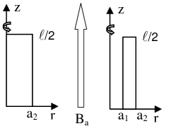
Figure 3: Cylinder and tube of external radius $a_{2}$, and length $\ell=6\leavevmode\nobreak\ a_{2}$ subjected to an axial magnetic induction $\mathbf{B}_{a}=B_{a}\hat{z}$. Only the region $0\leq r\leq{a_{2}}$ and $0\leq{z}\leq{\ell/2}$ is depicted for symmetry reasons.

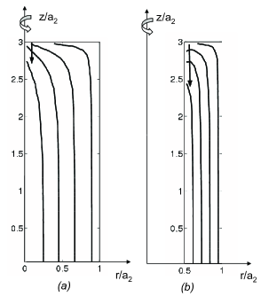
Figure 4: Cylinder (a) and tube (b) of external radius $a_{2}$, of length $\ell=6\leavevmode\nobreak\ a_{2}$ subjected to an axial magnetic field. The internal radius of the tube is $a_{1}=0.5\leavevmode\nobreak\ a_{2}$. The samples are characterized by field independent $J_{c}$ and $n$ values ($n=25$). As flux lines are symmetric about $z=0$ and $r=0$, only the region $0\leq{r}\leq{a_{2}}$ and $0\leq{z}\leq{\ell/2}$ is depicted. The contour curves show the flux fronts at $B_{a}=0.1,0.3,0.5,0.7\leavevmode\nobreak\ \mu_{0}H_{P}$ where $H_{P}$ is the field of full penetration.

Figure 4 shows a comparison of the simulated flux front for the cylinder (a) and for the tube (b) as a function of the applied magnetic induction. Here, the flux front corresponds to the locus of positions at which the current density rises to $J_{c}/2$. To label the front as a function of the applied induction, we have taken as a reference magnetic field the full penetration field, $H_{P}$, whose expression is given in (21) and (22), both for the bulk cylinder and for the tube. The flux front is depicted for different external magnetic inductions with $B_{a}/(\mu_{0}H_{P})=0.1,0.3,0.5,\leavevmode\nobreak\ \textrm{and}\leavevmode\nobreak\ 0.7$. We note that the front shapes are similar to those obtained by Navau et al. [34], which used an approximate method based on the minimization of the total magnetic energy to study the field penetration into bulk and hollow cylinders. Due to the finite length of the samples, the flux fronts are curved in the end region $z\cong\ell/2$. Remarkably, this curvature implies that the magnetic flux progresses faster towards $z=0$ along the inner boundary of the tube ($r=a_{1}$) than the magnetic flux penetrates the central region near $z=0$ in a bulk cylinder. Thus, two penetration mechanisms coexist for the tube: the magnetic field can penetrate either from the external boundary at $r=a_{2}$, as in the cylinder, or from the internal boundary at $r=a_{1}$, via the two openings.

Consider next the field lines  for the cylinder and for the tube submitted to axial fields equal to half of their respective field $H_{P}$ (see figure 5). The shape of the field lines in the region near $z=b$ are seen to be very different for the cylinder and for the tube. In particular, for the tube, the component $B_{z}$ is negative near the opening and close to the inner boundary, as seen in the dashed circle of figure 5(b). Such a behaviour is reminiscent of the field distribution found in the proximity of a thin ring [35, 36, 37, 38].

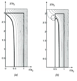
Figure 5: Cylinder (a) and tube (b) of external radius $a_{2}$ and length $\ell=6a_{2}$ subjected to an axial magnetic field. The samples are characterized by $J_{c}$ and $n$ values independent of the local magnetic induction ($n=25$). Only the region $0\leq{r}\leq{a_{2}}$ and $0\leq{z}\leq{\ell/2}$ is depicted. The applied induction is $0.5\leavevmode\nobreak\ \mu_{0}H_{P}$. The thick line represents the flux front ($J=J_{c}/2$) and the thin lines represent the magnetic field lines. One can observe negative components $B_{z}$ in the dashed circle of figure (b).

The existence of a negative $B_{z}$ inside the hollow part of the tube can be interpreted as follows. For an infinitely long tube, the magnetic field can only penetrate from the external surface and the field lines are parallel to the axis of the tube. As the length $\ell$ of the tube decreases, the flux lines spread out near $z=\ell$ due to demagnetization effects. As a result, shielding currents in the end region of the tube fail to totally shield the applied field and a non-zero magnetic field is admitted through the opening. The shielding currents flow in an extended region in the periphery of the superconductor. In the superconductor, ahead of the flux front, there is no shielding current and hence no electric field. Integrating Faraday-Lenz’s law along a contour lying in a non-penetrated region thus gives zero, meaning that the flux threaded by this contour must also be null. (As a reminder, the sample is cooled in zero-field.) Therefore, the magnetic flux due to the negative component $B_{z}$ near $r=a_{1}$ is there to cancel the positive flux that has been allowed in the hollow of the tube near the axis.

5.4 Uniformity of the field attenuation in a superconducting tube

Since magnetic flux can penetrate both through the outside surface and through the openings, it is therefore relevant to investigate how the magnetic induction varies in the hollow of the tube. Numerical simulations show that the variation of the field attenuation along the radius is much smaller than the variation along the $z$-axis. We thus concentrate on the latter and study the DC shielding factor, $DCSF$, as a function of $z$.

Figure 6 shows the variation of $DCSF$ along the $z$-axis as a function of the external induction $B_{a}$. The geometrical parameters are those of the sample studied experimentally and a $J_{c}(B)$ relation with the parameters of section 5.2 is used. As the curve $DCSF(z)$ is symmetric about $z=0$, only the portion $z>0$ is shown. Three different behaviours can be observed: in region $1$, the shielding factor is nearly constant; in region $2$, it starts decreasing smoothly; it falls off as an exponential in region $3$, which is roughly defined as the region for which $z>\ell/2-2a_{2}$.

A useful result is known for semi-infinite tubes made of type-I superconductor and subjected to a weak axial field. In the Meissner state, the magnitude of the internal induction, $B_{\mathrm{in}}$, decreases from the extremity of the tube [39] as

$$B_{\mathrm{in}}\propto\mathrm{e}^{-C(\ell/2-z)/a_{1}},$$ (24)

where $a_{1}$ is the inner radius, and $C\approx 3.83$ is the first zero of the Bessel function of the first kind $J_{1}(x)$. This result holds for $\ell/2-z\gg a_{1}$ and implies that the shielding factor increases as an exponential of $\ell/2-z$. An exponential dependence has also been measured in some HTS materials for applied fields above $H_{c1}$ [14, 15]. Other measurements [16] in similar conditions have shown instead a uniform shielding factor in a region around the center of the tube.

From the simulation results we see that both behaviours can actually be observed in a type-II tube, provided the ratio $\ell/\bar{a}$ is large. For the sample studied in this paper, this ratio is equal to $\ell/\bar{a}\sim 11$. The exponential falloff approximately follows the law $DCSF(z)\sim\exp(C(\ell/2-z)/a_{1})$ (black solid line) for the lowest fields only, but appears much softer for the larger magnitudes $B_{a}$. This behaviour can be attributed to the fact that as $B_{a}$ increases, the region near $z=\ell/2$ becomes totally penetrated (see figure 4) and the “effective” length of the tube decreases. It leads in turn to a reduction of the distance to the extremity, $\ell/2-z$, which therefore softens the falloff of the shielding factor.

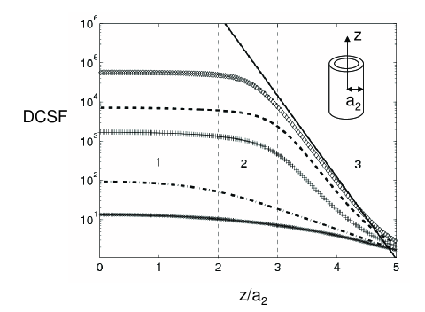
Figure 6: Simulated variation of the DC shielding factor along the $z$-axis for increasing applied inductions. From top to bottom : $B_{a}/B_{\mathrm{lim}}=0.8,0.9,1,1.05,\>\texttt{and}\>1.1$. The threshold $B_{\mathrm{lim}}$ is determined as the maximum applied induction for which the shielding factor is higher than 60 dB. The geometry is identical to that of the sample studied experimentally. The black solid line is the equation $DCSF(z)=e^{C(\ell/2-z)/a_{1}}$ (see text). For symmetry reasons, only the upper half of the tube is shown.

The two behaviours — a nearly constant shielding factor and an exponential decrease of this factor — can be associated with the two mentioned penetration mechanisms. For the part of the flux that penetrates via the openings, we expect the shielding factor to increase as an exponential of $(\ell/2-z)$ as one moves away from the extremity. This is the behaviour observed in type-I shields, for which no flux can sweep through the side wall if $d\gg\lambda$, where $\lambda$ denotes the London penetration depth. By contrast, in the centre region, for a tube with a large $\ell/\bar{a}$ ratio, the flux penetrating via the openings is vanishingly small and flux penetration through the walls prevails. This leads to the nearly constant shielding factor observed in region $1$. As the ratio $\ell/\bar{a}$ increases, flux penetration through the wall strengthens. As a result, the plateau region increases in size as is confirmed in figure 7, which shows $DCSF(z)$ for six different lengths $\ell/a_{2}$ (the outer radius and the width $d=a_{2}-a_{1}=0.2a_{2}$ are kept fixed) and for $B_{a}=0.85\leavevmode\nobreak\ B_{\mathrm{lim}}$. Note that the plateau of the shielding factor disappears for the smallest ratios $\ell/\bar{a}$ (for $\ell\leq 6a_{2}$) as for these ratios, flux penetration through the openings competes with that through the wall.

This last example shows that it is important to distinguish $B_{\mathrm{lim}}$, which we have defined as the maximum induction for which $DCSF$ is larger than 60 dB, from $\mu_{0}H_{P}$, which corresponds to the full penetration of the sample. In fact, for $\ell<6a_{2}$, the attenuation falls below 60 dB before the sample is full penetrated. If $\ell$ is further reduced, $\ell\leq 2a_{2}$, it is actually not possible to define an induction $B_{\mathrm{lim}}$, as $DCSF$ is lower than 60 dB for any applied inductions. Therefore, the interest of using short open HTS tubes for magnetic shielding applications is very limited.

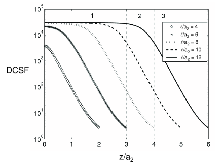
Figure 7: Evolution of the DC shielding factor along the axis for different lengths, $\ell$. The internal and external radii, $a_{1}$ and $a_{2}$, are kept fixed ($a_{1}=0.8\leavevmode\nobreak\ a_{2}$). The applied induction is $B_{a}=0.85\leavevmode\nobreak\ B_{\mathrm{lim}}$.

When $\ell\geq 6a_{2}$, the value of $B_{\mathrm{lim}}$ is very close to the applied field for which the sample is fully penetrated, as the main penetration mechanism is the non-linear diffusion through the superconducting wall. To evaluate $B_{\mathrm{lim}}$, one could then use (22), which for $\ell\geq 6a_{2}$, is close to $H_{P\infty}=J_{c}d$ . However, this formula can be misleading for understanding the influence of the wall thickness, $d$. Expressions (22) or $H_{P\infty}=J_{c}d$ were established ignoring the variation of $J_{c}$ with $B$ and show a linear dependence of $B_{\mathrm{lim}}$ as a function of $d$. However, the decrease of $J_{c}$ with the local induction yields a softer dependence as can be seen in (20). There, $B_{\mathrm{lim}}\approx B_{\mathrm{lim},\infty}$ is linear in $d$ only for thicknesses $d$ much smaller than $B_{1}/(2\mu_{0}J_{c0})\approx 0.1\leavevmode\nobreak\ \mathrm{mm}$, but grows as $\sqrt{d}$ for larger thicknesses if one takes the $J_{c0}$ and $B_{1}$ parameters of section 5.2. Thus, if one wants to shield high magnetic inductions (larger than $100\leavevmode\nobreak\ \mathrm{mT}$) with a superconductor similar to that described in section 3, unreasonnably thick wall thicknesses are required. In this case, it is advisable to first reduce the field applied to the superconductor by placing a ferromagnetic screen around it.

A final remark concerns the effect of the width of the superconducting wall, $d$, on the spatial dependence of $DCSF$. If $d$ is increased while the ratio $B_{a}/B_{\mathrm{lim}}$ is kept fixed, the shielding factor increases in magnitude but its $z$-dependence remains qualitatively the same.

In this section, we used a quasistatic field. The results concerning the spatial variation of the field attenuation are expected to be still valid in the case of an AC field.

6 Magnetic shielding in the AC mode

The sensing coil of the setup described in section 3 can move along the axis of the sample. In this section, we first present the measured variation of the AC shielding factor along the axis of the tube and compare it to numerical simulations for which an AC applied induction is used. We also measure the frequency response and interpret the results with scaling laws arising from the constitutive law $E\propto J^{n}$.

6.1 Experimental results

The variations of the measured AC shielding factor $ACSF$ defined in (15), along the axis of the sample studied experimentally for a fixed frequency and varying amplitudes of the applied field are shown in figure 8 (filled symbols). Apart from the upper curve of figure 8 corresponding to $B_{a,RMS}=10.8\leavevmode\nobreak\ \mathrm{mT}$, we observe a nearly constant measured shielding factor in the central region . Going further to the extremity of the tube, near $z=5a_{2}$, $ACSF$ decreases as an exponential.

Figure 9 (filled symbols) shows a measurement of the AC shielding factor, $ACSF$, as a function of frequency for two applied magnetic inductions when the magnetic sensor is placed at the centre of the sample. The frequency dependence appears to follow a power law.

Figure 10 shows the evolution of the AC shielding factor measured at the centre of the tube at a fixed frequency $f=103\leavevmode\nobreak\ \mathrm{Hz}$ and for varying RMS values of the applied induction. The shielding factor decreases with $B_{a,RMS}$.

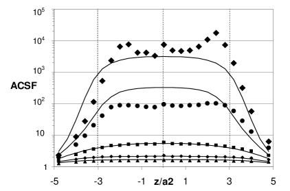
Figure 8: Variation of the AC shielding factor along the axis of the sample, at a frequency $f=103\leavevmode\nobreak\ \mathrm{Hz}$. Filled symbols : measurement. Continuous lines : simulation. From top to bottom: $B_{a,RMS}=10.8,\,12,\,13.4,\,15.3,\,\texttt{and}\,16.6\leavevmode\nobreak\ \mathrm{mT}$.

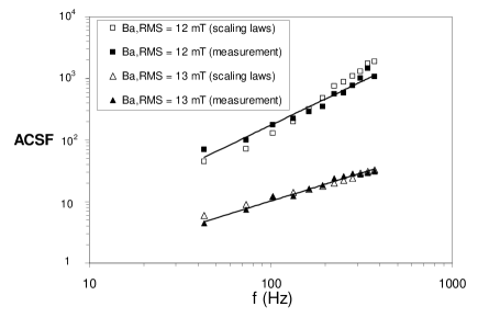
Figure 9: AC shielding factor versus frequency. The filled symbols come from a direct measurement and the open symbols correspond to an estimation based on scaling laws (see text). The two lines show that the variation of the AC shielding factor with the frequency is close to a power law.

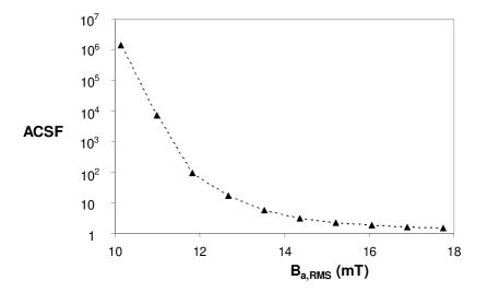
Figure 10: Measured AC shielding factor at the centre of the sample versus the RMS value of the applied magnetic induction $B_{a,RMS}$. Its frequency is kept fixed at $f=103\leavevmode\nobreak\ \mathrm{Hz}$.

6.2 Uniformity of the field attenuation

The solid lines of figure 8 represent the simulated $ACSF$ for the applied inductions used during the measurement. As in the DC case, we observe a constant shielding factor around the centre $z=0$ of the tube whereas $ACSF$ falls off exponentially near the opening ends $z=5a_{2}$. Remarkably, one can observe the relative good quantitative agreement between simulated and experimental results of figure 8. For $B_{a,RMS}=10.8\leavevmode\nobreak\ \mathrm{mT}$, local variations of the measured $ACSF$ can be observed for $\left|z\right|<3$. In particular, the maximum shielding factor is no longer located at the centre of the tube, and shielding appears to be asymmetric in $z$. For higher values of the applied magnetic induction, the maximum $ACSF$ lies at $z=0$ and shielding recovers its symmetry about the centre. These effects are supposed to be due to non-uniform superconducting properties.

6.3 Scaling laws and frequency response

The strong non-linearity of the constitutive law $E=E_{c}(J/J_{c})^{n}$ gives rise to frequency scaling laws with $n-$dependent power exponents [19]. The scaling laws can be obtained by changing the time unit in Maxwell’s equations (5) and (6) by a factor $c>0$, $t\mapsto t_{\mathrm{new}}={t/c}$. Given a solution with a current density $J(\mathbf{r},t)$, an applied induction $B_{a}(\mathbf{r},t)$, and a total induction $B(\mathbf{r},t)$, new solutions can be found that satisfy

$$J_{\mathrm{new}}(\mathbf{r},t_{\mathrm{new}}) = J(\mathbf{r},t)\,c^{1/(n-1)},$$ (25)

$$B_{\mathrm{new}}(\mathbf{r},t_{\mathrm{new}}) = B(\mathbf{r},t)c\,^{1/(n-1)},$$ (26)

$$B_{a,\mathrm{new}}(\mathbf{r},t_{\mathrm{new}}) = B_{a}(\mathbf{r},t)\,c^{1/(n-1)}.$$ (27)

Transposed to the frequency domain, these relations imply that if the frequency of the applied field is multiplied by a factor $c$, then the current density and the magnetic induction are rescaled by the factor $c^{1/(n-1)}$. In particular, if one knows the $ACSF$ corresponding to the applied induction $B_{a}$ at the frequency $f$, $ACSF(Ba,f)$, one can deduce the $ACSF$ corresponding to the magnetic induction $B_{a,\mathrm{new}}$ at the frequency $f_{\mathrm{new}}=c\,f$ by using:

$$ACSF(B_{a,\mathrm{new}},f_{\mathrm{new}})=ACSF(B_{a},f),$$ (28)

as $ACSF$ is the ratio of two magnetic inductions (see (15)) and is thus invariant under scaling. Then, the frequency dependence of $ACSF$ in figure 9 can be reproduced as follows using these scaling laws. First, we approximate the curve of figure 10 by piecewise exponentials, which gives $ACSF(B_{a},103\leavevmode\nobreak\ \mathrm{Hz})$. Second, we use (28) and write:

$$ACSF(12\leavevmode\nobreak\ \mathrm{mT},f_{\mathrm{new}})=ACSF(B_{a},103\leavevmode\nobreak\ \mathrm{Hz}),$$ (29)

with

$$B_{a} = B_{a,\mathrm{new}}\,c^{-1/(n-1)}$$ (30)

$$= 12\leavevmode\nobreak\ \mathrm{mT}\left(\frac{103}{f_{\mathrm{new}}}\right)^{1/(n-1)}$$ (31)

Hence, the variations with respect to $B_{a}$ in figure 10 can be translated into frequency variations at a fixed induction. This gives the upper curve of figure 9 (open symbols) for which we used $n=25$. The lower curve is obtained by fixing $B_{a,\mathrm{new}}$ to $13\leavevmode\nobreak\ \mathrm{mT}$. This construction thus demonstrates that the frequency variation intrinsically arises from scaling laws.

The detailed construction relies on a specific value of the creep exponent $n$, which we have taken here to be equal to $n=25$ and independent on $B$. Analysing the frequency dependence with scaling laws thus also serves the purpose of determining the value of $n$ that best fits experimental data. A HTS shield characterized by a lower $n$ value would present a more pronounced frequency dependence of the shielding factor.

One may wonder on the role played by the increased dissipation, due to the motion of vortices, as frequency is increased. Such dissipation can lead to a temperature rise, a decrease of the critical current density, and thus a decrease of the shielding factor. Nevertheless, it appears from figure 9 that the temperature increase must remain small in the frequency window investigated in our experiment ($43\leavevmode\nobreak\ \mathrm{Hz}-373\leavevmode\nobreak\ \mathrm{Hz}$), as no significant reduction of $ACSF$ can be observed in that frequency range. One may equally wonder on the role played by the different harmonics of the internal magnetic induction. For the applied fields we consider here, the fundamental component strongly dominates the higher harmonics. As as consequence, the curves of figures 9, and 10 are not significantly affected if one takes the RMS value of the total internal magnetic induction, rather than its fundamental component, to define the shielding factor in the AC mode.

7 Conclusions

We have presented a detailed study of the magnetic shielding properties of a polycrystalline Bi-2223 superconducting tube subjected to an axial field. We have measured the field attenuation with high sensitivity for DC and AC source fields, and have confronted data with computer modelling of the field distribution in the hollow of the tube. The numerical model is based on the algorithm described in [19], which is easy to implement on a personal computer. Our study allows us to detail the variation of the shielding factor along the axis, interpret it in terms of the penetration mechanisms, and take into account flux creep and its effect on the frequency dependence. To our knowledge, it is the first study which systematically describes the spatial and frequency variations of the shielding factor in the hollow of a HTS tube.

Our main findings can be summarized as follows.

• A HTS tube can efficiently shield an axial induction below a threshold induction $B_{\mathrm{lim}}$. For our commercial sample, $B_{\mathrm{lim}}=14\leavevmode\nobreak\ \mathrm{mT}$. The threshold induction $B_{\mathrm{lim}}$ increases with the ratio $\ell/\bar{a}$, the thickness of the tube, and depends on the exact $J_{c}(B)$ dependence ($\ell$ is the length of the tube and $\bar{a}$ is the mean radius). When the length of the tube decreases, $B_{\mathrm{lim}}$ can be strongly reduced because of demagnetizing effects.

• There are two penetration mechanisms in a HTS tube in the parallel geometry: one from the external surface of the tube, and one from the opening ends, the latter mechanism being suppressed for long tubes. These two mechanisms lead to a spatial variation of the shielding factor along the axis of the tube. In a zone extending between $z=0$ (centre of the tube) and $z=\ell/2-3a_{2}$, the shielding factor is constant when $\ell>6a_{2}$ ($a_{2}$ is its external radius). Then it decreases as an exponential as one moves towards the extremity of the tube. As a consequence of this spatial dependence, no zone with a constant shielding factor exists for small tubes ($\ell<6a_{2}$).

• The shielding factor increases with the frequency of the field to shield, following a power law. This dependence can be explained from scaling laws arising from the constitutive law $E\propto J^{n}$.

In practice, a tube of a Bi-2223 ceramic can thus be used to effectively shield an axial field at low frequencies. A sample with an outer radius $a_{2}=1.8\leavevmode\nobreak\ \mathrm{mm}$, a length $\ell>6a_{2}$, a thickness $d=1.5\leavevmode\nobreak\ \mathrm{mm}$, and with superconducting properties similar to the ones of our sample (table 1), strongly attenuates magnetic inductions lower than $B_{\mathrm{lim}}=14\leavevmode\nobreak\ \mathrm{mT}$ at $77\leavevmode\nobreak\ \mathrm{K}$. The shielding factor is nearly constant and larger than $10^{3}$ (60 dB) in the region $|z|<\ell/2-3a_{2}$ if the applied induction is lower than $0.9\leavevmode\nobreak\ B_{\mathrm{lim}}$.

8 Acknowlegment

E.H. Brandt is gratefully acknowledged for useful discussions. A.F. Gerday and D. Bajusz are also acknowledged for their experimental support. This research was supported in part by a ULg grant (Conseil de la Recherche support through project “Fonds spéciaux” (C-06/03)) and by the Belgian F.N.R.S (grant from FRFC: 1.5.115.03).