A geometric growth model interpolating between regular and small-world networks

Abstract

We propose a geometric growth model which interpolates between one-dimensional linear graphs and small-world networks. The model undergoes a transition from large to small worlds. We study the topological characteristics by both theoretical predictions and numerical simulations, which are in good accordance with each other. Our geometrically growing model is a complementarity for the static WS model.

[A,D,B]Zhongzhi Zhang [A,D,C]Shuigeng Zhou Corresponding author. [A,D]Zhiyong Wang [A,D]Zhen Shen

1 Introduction

Many real-life systems display both a high degree of local clustering and the small-world effect [1, 2, 3, 4, 5]. Local clustering characterizes the tendency of groups of nodes to be all connected to each other, while the small-world effect describes the property that any two nodes in the system can be connected by relatively short paths. Networks with these two characteristics are called small-world networks.

In the past few years, in order to describe real-life small-world networks, a number of models have been proposed. The first and the most widely-studied model is the simple and attractive small-world network model of Watts and Strogatz (WS model) [6], which triggered a sharp interest in the studies of the different properties of small-world networks such as the WS model or its variations. Many authors tried to find more rigorous analytical results on the properties of either the WS model or on its variants that were easier to analyze or captured new aspects of small-worlds [7, 8, 9, 10, 11, 12, 13, 14]. The WS model and its variants may provide valuable insight into some real-life networks showing how real-world systems are shaped. However, the small-world effect is much more general, it is still an active direction of research to explore other mechanisms producing small-world networks.

In real systems, a series of microscopic events shape the network evolution, including addition or removal of a node and addition or removal of an edge [16, 17, 18, 19, 20]. In addition, the number of nodes in some real-life networks increases exponentially with time. The World Wide Web, for example, has been increasing in size exponentially from a few thousand nodes in the early 1990s to hundreds of millions today. To our knowledge, all previous models of small-world networks either are static (not growing) or have focused solely on addition of nodes and edges one by one. Therefore, it is interesting to establish a exponentially growing network model and investigate the effect of more events, such as removal of edges, on the topological features.

In this paper, we present a simple geometric growth network model controlled by a tunable parameter $q$, where existing edges can be removed. As in the WS model, by tuning parameter $q$, the model undergoes a phase transition transition with increasing number of nodes from a “large-world” regime in which the average path length increases linearly with system size, to a “small-world” one in which it increases logarithmically. We study analytically and numerically the structural characteristics, all of which depend on the parameter $q$.

Our model is probable not as much a model of a real-world system as an example of vast variety of structure within the class of networks defined by a degree distribution, but it is the first growing model that exhibits the similar phenomena as the famous WS model. Thus, it may be helpful for establishing more realistic growing small-world models of real-life systems in future.

2 The network model

The network model is generated by decimating semi-ring, which is constructed in an iterative way as shown in Fig. 1. We denote our network after $t$ ($t\geq 0$) time steps by $N_{t}$. The network starts from an initial state ($t=0$) of two nodes, which are distributed on both ends of a semi-ring and connected by one edge. For $t\geq 1$, $N_{t}$ is obtained from $N_{t-1}$ as follows: for each existing internode interval along the semi-ring of $N_{t-1}$, a new node is added and connected to its both end nodes; at the same time, for each existing internode interval, with probability $q$, we remove the edge linking its two end nodes, previously existing at step $t-1$. The growth process is repeated until the network reaches the desired size.

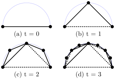
Figure 1: Scheme of the growing network for the case of $q=0.5$, showing the first four steps of the iterative process. The dashed lines denote the removed edges.

When $q=1$, the network is reduced to the one-dimension linear chains. For $q=0$, no edge are deleted, and the network grows deterministically, which allows one exactly calculate its topological properties. As we will show below that in the special of $q=0$ the network is small-world. Thus, varying $q$ in the interval (0,1), we can study the crossover between the one-dimension regular linear graph and the small-world network.

Now we compute the number of nodes and edges in $N_{t}$. We denote the number of newly added nodes and edges at step $t$ by $L_{v}(t)$ and $L_{e}(t)$, respectively. Thus, initially ($t=0$), we have $L_{v}(0)=2$ nodes and $L_{e}(0)=1$ edges in $N_{0}$. Let $N_{c}(t)$ denote the total number of internode intervals along the semi-ring at step $t$, then $N_{c}(0)=1$. By construction, we have $L_{v}(t)=N_{c}(t-1)$ for arbitrary $t\geq 1$. Note that, when a new node is added to the network, an interval is destroyed and replaced by two new intervals, hence we have the following relation: $N_{c}(t)=2\,N_{c}(t-1)$. Considering the initial value $N_{c}(0)=1$, we can easily get $N_{c}(t)=L_{v}(t+1)=2^{t}$. On the other hand, the addition of each new node leads to two new edges and one old edge removed with probability $q$, which follows that $L_{e}(t)=(2-q)\,L_{v}(t)=(2-q)\,2^{t-1}$. Therefore, the number of nodes $V_{t}$ and the total of edges $E_{t}$ in $N_{t}$ is

$$V_{t}=\sum_{t_{j}=0}^{t}L_{v}(t_{j})=2^{t}+1$$ (1)

and

$$E_{t}=\sum_{t_{j}=0}^{t}L_{e}(t_{j})=(2-q)\,2^{t}+q-1,$$ (2)

respectively. The average node degree is then

$$\langle k\rangle_{t}=\frac{2E_{t}}{V_{t}}=(4-2q)-\frac{3-2q}{2^{t}+1}$$ (3)

For large $t$ and any $q$, it is small and approximately equal to $4-2q$. Notice that many real-life networks are sparse in the sense that the number of edges in the network is much less than $V_{t}(V_{t}-1)/2$, the number of all possible edges [2, 3, 4].

3 Structural properties

Below we will find that the tunable parameter $q$ controls all the relevant properties of the model, including degree distribution, clustering coefficient, and average path length.

3.1 Degree distribution

The degree distribution $P(k)$ is defined as the probability that a randomly selected node has exactly $k$ edges. For $q=1$, all nodes, except the initial two nodes created at step 0, have the same number of connections 2, the network exhibits a completely homogeneous degree distribution.

Next we focus the case $0\leq q<1$. Let $k_{i}(t)$ denote the degree of node $i$ at step $t$. If node $i$ is added to the network at step $t_{i}$ ($t_{i}\geq 1$), then, by construction, $k_{i}(t_{i})=2$. In each of the subsequent time steps, there are two intervals with one at either side of $i$. Each of the two intervals will create a new node connected to $i$, and each edge connecting the end nodes of the intervals could be considered to be deleted with probability $q$. Then the degree $k_{i}(t)$ of node $i$ satisfies the relation

$$k_{i}(t)=k_{i}(t-1)+2(1-q).$$ (4)

It should be mentioned that Eq. (4) does not hold true for the two initial nodes created at step 0. But when the network becomes large, these few initial nodes have almost no effect on the structural characteristics. Considering the initial condition $k_{i}(t_{i})=2$, Eq. (4) becomes

$$k_{i}(t)=2+2(1-q)(t-t_{i}).$$ (5)

The degree of each node can be obtained explicitly as in Eq. (5), and we see that this degree increases at each iteration. So it is convenient to obtain the cumulative distribution [4]

$$P_{cum}(k)=\sum_{k^{\prime}=k}^{\infty}P(k^{\prime})$$ (6)

which is the probability that the degree is greater than or equal to $k$. For some networks whose degree distributions have exponential tails: $P(\tilde{k})\sim e^{-\tilde{k}/\kappa}$, cumulative distribution also has an exponential expression with the same exponent:

$$P_{cum}(\tilde{k})=\sum_{k^{\prime}=\tilde{k}}^{\infty}P(k^{\prime})\sim\sum_{k^{\prime}=\tilde{k}}^{\infty}e^{-k^{\prime}/\kappa}\sim e^{-\tilde{k}/\kappa}$$ (7)

This makes exponential distributions particularly easy to spot experimentally, by plotting the corresponding cumulative distributions on semilogarithmic scales.

Using Eq. (5), we have $P_{cum}(k)=\sum_{k^{\prime}=k}^{\infty}P(k)=P\left(t^{\prime}\leq\tau=t-\frac{k-2}{2(1-q)}\right)$. Hence

$$P_{cum}(k) = \sum_{t^{\prime}=0}^{\tau}\frac{L_{v}(t^{\prime})}{V_{t}}$$ (8)

$$= \frac{2}{2^{t}+1}+\sum_{t^{\prime}=1}^{\tau}\frac{2^{t^{\prime}-1}}{2^{t}+1}$$

$$= 2^{-\frac{k-2}{2(1-q)}}$$

The cumulative distribution decays exponentially with $k$. Thus the resulting network is an exponential network. Note that many small-world networks including the WS model belong to this class [9].

Figure 2: Semilogarithmic graph of cumulative degree distribution of the network $N_{17}$ for different $q$. All the networks have size 131073. The solid lines are the analytic calculation values given by Eq. (8).

In Fig. 2, we report the simulation results of the degree distribution for several values of $q$. From Fig. 2, we can see that the degree distribution decays exponentially, in agreement with the analytical results and supporting a relatively homogeneous topology similar to most small-world networks [9, 12, 13, 14].

3.2 Clustering coefficient

By definition, clustering coefficient [6] $C_{i}$ of a node $i$ is the ratio of the total number $e_{i}$ of edges that actually exist between all $k_{i}$ its nearest neighbors and the number $k_{i}(k_{i}-1)/2$ of all possible edges between them, i.e. $C_{i}=2e_{i}/[k_{i}(k_{i}-1)]$. The clustering coefficient $\langle C\rangle$ of the whole network is the average of all individual $C_{i}^{\prime}s$.

For the case of $q=1$, the network is a one-dimensional chain, the clustering coefficient of an arbitrary node and their average value are both zero.

For the case of $q=0$, using the connection rules, it is straightforward to calculate exactly the clustering coefficient of an arbitrary node and the average value for the network. When a new node $i$ joins the network, its degree $k_{i}$ and $e_{i}$ is $2$ and $1$, respectively. Each subsequent addition of a link to that node increases both $k_{i}$ and $e_{i}$ by one. Thus, $e_{i}$ equals to $k_{i}-1$ for all nodes at all steps. So one can see that there is a one-to-one correspondence between the degree of a node and its clustering. For a node $v$ of degree $k$, the exact expression for its clustering coefficient is $\frac{2}{k}$, which has been also been obtained in other models [12, 13, 14, 21]. This expression indicates that the local clustering scales as $C(k)\sim k^{-1}$. It is interesting to notice that a similar scaling has been observed empirically in several real-life networks [22].

Clearly, the number $n(C,t)$ of nodes with clustering coefficient $C=1$, $\frac{1}{2}$, $\frac{1}{3}$, $\cdots$, $\frac{1}{t-1}$, $\frac{1}{t}$, $\frac{2}{t+1}$ , is equal to $L_{v}(t)$, $L_{v}(t-1)$, $L_{v}(t-2)$, $\cdots$, $L_{v}(2)$, $L_{v}(1)$, $L_{v}(0)$, respectively. Therefore, the clustering coefficient spectrum of nodes is discrete. Using this discreteness, it is convenient to work with the cumulative distribution of clustering coefficient [21] as

$$W_{\rm cum}(C)=\frac{1}{V_{t}}\sum_{C^{\prime}\leq C}n(C^{\prime},t)=2\left(\frac{1}{2}\right)^{C},$$ (9)

where $C$ and $C^{\prime}$ are the points of the discrete spectrum. The average clustering coefficient $\langle C\rangle_{t}$ can be easily obtained for arbitrary $t$,

$$\langle C\rangle_{t} = \frac{1}{V_{t}}\left[\sum_{i=1}^{t}\frac{1}{i}\cdot L_{v}(t+1-i)+\frac{2}{t+1}\cdot L_{v}(0)\right]$$ (10)

$$\simeq 1\cdot\frac{1}{2}+\frac{1}{2}\cdot\frac{1}{2^{2}}+\frac{1}{3}\cdot\frac{1}{2^{3}}+$$

$$\hskip 30.00005pt\cdots+\frac{1}{t}\cdot\frac{1}{2^{t}}+\frac{2}{t+1}\cdot\frac{2}{2^{t}}$$

$$= \sum_{i=1}^{t}\frac{1}{i}\left(\frac{1}{2}\right)^{i}+\frac{2}{t+1}\cdot\frac{2}{2^{t}}$$

For infinite $t$, $\langle C\rangle=-\ln(1-\frac{1}{2})=\ln 2$ , which approaches to a constant value 0.6931, and so the clustering is high.

In the range $0<q<1$, it is difficult to derive an analytical expression for the clustering coefficient either for an arbitrary node or for their average. In order to obtain the result of the clustering coefficient $C$ of the whole network, we have performed extensive numerical simulations for the full range of $q$ between 0 and 1. Simulations were performed for network $N_{17}$ with size $131073$, averaging over 20 network samples for each value of $q$.

Figure 3: The clustering coefficient $C$ of the whole network as a function of $q$.

In Fig. 3, we plot the clustering coefficient $C$ as a function of $q$. It is obvious that $C$ decreases continuously with increasing $q$. As $q$ increases from 0 to 1, $C$ drops almost linearly from 0.6931 to 0. Note that although the clustering coefficient $C$ changes linearly for all $q$, we will show below that in the large limit of $q$, the average path length changes exponentially as $q$ . This is different from the phenomenon observed in the WS model where $C$ remains practically unchanged in the process of the network transition to a small world.

3.3 Average Path Length

We represent all the shortest path lengths of $N_{t}$ as a matrix in which the entry $d_{ij}$ is the geodesic path from node $i$ to node $j$, where geodesic path is one of the paths connecting two nodes with minimum length. A measure of the typical separation between two nodes in $N_{t}$ is given by the average path length $\bar{d}_{t}$, also known as characteristic path length, defined as the mean of geodesic lengths over all couples of nodes:

$$\bar{d}_{t}=\frac{S_{t}}{V_{t}(V_{t}-1)/2}\,,$$ (11)

where

$$S_{t}=\sum_{i\neq j,\,\,i\in N_{t},\,j\in N_{t}}d_{ij}$$ (12)

denotes the sum of the chemical distances between two nodes over all pairs. For general $q$, there are some difficulties in obtaining a closed formula for $\bar{d}_{t}$. For $q=1$ and $q=0$, the networks are deterministic, which allows one to calculate $\bar{d}_{t}$ analytically.

3.3.1 Case of $q=1$

For this particular case, the network is a linear chain (graph) which has two nodes with degree 1 at both ends of the chain and $V_{t}-2$ nodes with degree 2 in the middle. For convenience, we denote the total distances between all pair of nodes and average path length of a linear chain with $n$ nodes as $\sigma(n)$ and $l(n)$, respectively. We label each node in the linear graph with size $n$ from one end to the other as $v=1,2,\cdots,n-1,n.$ Then we have the following equation:

$$\sigma(n+1)=\sigma(n)+\theta_{n},$$ (13)

where $\theta_{n}$ is defined as

$$\theta_{n}=\sum_{i=1}^{n}d_{i(n+1)}=\sum_{i=1}^{n}\,i=\frac{n(n+1)}{2}.$$ (14)

Then the solution of Eq. (13) is

$$\sigma(n) = \sigma(2)+\sum_{m=2}^{n-1}\theta_{m}=1+\sum_{m=2}^{n-1}\,\frac{m(m+1)}{2}$$ (15)

$$= 1+\frac{1}{2}\,\left(\sum_{m=2}^{n-1}m^{2}+\sum_{m=2}^{n-1}m\right)$$

$$= \frac{n(n-1)(n+1)}{6}.$$

Thus

$$l(n)=\frac{\sigma(n)}{n(n-1)/2}=\frac{n+1}{3},$$ (16)

which increases linearly with network size.

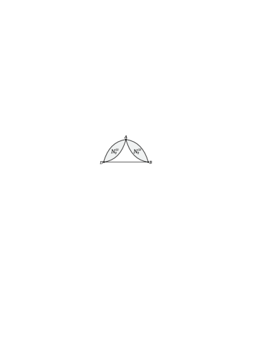
Figure 4: For $q=0$, the network after $t+1$ step iterations, $N_{t+1}$, is composed of two copies of $N_{t}$ denoted as $N_{t}^{(1)}$ and $N_{t}^{(2)}$, which are connected to each other as above.

3.3.2 Case of $q=0$

In the special case, the network has a self-similar structure that allows one to calculate $\bar{d}_{t}$ analytically, based on a similar method as that proposed in [23]. As shown in Fig. 4, the network $N_{t+1}$ may be obtained by joining $2$ copies of $N_{t}$ , which are labeled as $N_{t}^{(\alpha)}$, $\alpha=1,2$. Then we can write the sum $S_{t+1}$ as

$$S_{t+1}=2\,S_{t}+\Delta_{t}\,,$$ (17)

where $\Delta_{t}$ is the sum over all shortest paths whose endpoints are not in the same $N_{t}$ branch. The solution of Eq. (17) is

$$S_{t}=2^{t-1}S_{1}+\sum_{m=1}^{t-1}2^{t-m-1}\Delta_{m}\,.$$ (18)

The paths that contribute to $\Delta_{t}$ must all go through at least one of the $3$ edge nodes ($A$, $B$, $D$) at which the two $N_{t}$ branches are connected. Below we give the analytical expression for $\Delta_{t}$, called the crossing paths.

We define

$$d_{t}^{\text{tot}} \equiv\sum_{i\in N_{t}^{(1)}}d_{iA}\,,$$

$$d_{t}^{\text{near}} \equiv\sum_{\begin{subarray}{c}i\in N_{t}^{(1)}\\ d_{iA}<d_{iD}\end{subarray}}d_{iA}\,,\qquad V_{t}^{\text{near}}\equiv\sum_{\begin{subarray}{c}i\in N_{t}^{(1)}\\ d_{iA}<d_{iD}\end{subarray}}1\,,$$

$$d_{t}^{\text{mid}} \equiv\sum_{\begin{subarray}{c}i\in N_{t}^{(1)}\\ d_{iA}=d_{iD}\end{subarray}}d_{iA}\,,\qquad V_{t}^{\text{mid}}\equiv\sum_{\begin{subarray}{c}i\in N_{t}^{(1)}\\ d_{iA}=d_{iD}\end{subarray}}1\,,$$

$$d_{t}^{\text{far}} \equiv\sum_{\begin{subarray}{c}i\in N_{t}^{(1)}\\ d_{iA}>d_{iD}\end{subarray}}d_{iA}\,,\qquad V_{t}^{\text{far}}\equiv\sum_{\begin{subarray}{c}i\in N_{t}^{(1)}\\ d_{iA}>d_{iD}\end{subarray}}1\,,$$ (19)

so that $d_{t}^{\text{tot}}=d_{t}^{\text{near}}+d_{t}^{\text{mid}}+d_{t}^{\text{far}}$ and $V_{t}=V_{t}^{\text{near}}+V_{t}^{\text{mid}}+V_{t}^{\text{far}}$. By symmetry $V_{t}^{\text{near}}=V_{t}^{\text{far}}$. Thus,

$$\Delta_{t} =\sum_{\begin{subarray}{c}i\in N_{t}^{(1)},\,\,j\in N_{t}^{(2)}\\ i,j\neq A\end{subarray}}d_{ij}=\sum_{\begin{subarray}{c}i\in N_{t}^{(1)},\,\,j\in N_{t}^{(2)}\\ i,j\neq A,\,\,d_{iA}\leq d_{iD}\end{subarray}}(d_{iA}+d_{Aj})$$

$$\quad+\sum_{\begin{subarray}{c}i\in N_{t}^{(1)},\,\,j\in N_{t}^{(2)},\,\,i,j\neq A\\ d_{iA}>d_{iD},\,\,d_{jA}\leq d_{jB}\end{subarray}}(d_{iA}+d_{Aj})$$

$$\quad+\sum_{\begin{subarray}{c}i\in N_{t}^{(1)},\,\,j\in N_{t}^{(2)},\,\,i,j\neq A\\ d_{iA}>d_{iD},\,\,d_{jA}>d_{jB}\end{subarray}}(d_{iD}+1+d_{Bj})$$

$$=\sum_{\begin{subarray}{c}i\in N_{t}^{(1)},\,\,i\neq A\\ d_{iA}\leq d_{iD}\end{subarray}}\left[(V_{t}-1)d_{iA}+d_{t}^{\text{tot}}\right]$$

$$+\sum_{\begin{subarray}{c}i\in N_{t}^{(1)},\,\,i\neq A\\ d_{iA}>d_{iD}\end{subarray}}\left[(V_{t}^{\text{near}}+V_{t}^{\text{mid}}-1)d_{iA}+d_{t}^{\text{near}}+d_{t}^{\text{mid}}\right]$$

$$\quad+\sum_{\begin{subarray}{c}i\in N_{t}^{(1)},\,\,i\neq A\\ d_{iA}>d_{iD}\end{subarray}}\left[V_{t}^{\text{near}}(d_{iD}+1)+d_{t}^{\text{near}}\right]$$

$$=(V_{t}-1)(d_{t}^{\text{near}}+d_{t}^{\text{mid}})+(V_{t}^{\text{near}}+V_{t}^{\text{mid}}-1)d_{t}^{\text{tot}}$$

$$\quad+(V_{t}^{\text{near}}+V_{t}^{\text{mid}}-1)d_{t}^{\text{far}}+V_{t}^{\text{near}}(d_{t}^{\text{near}}+d_{t}^{\text{mid}})$$

$$\quad+V_{t}^{\text{near}}(d_{t}^{\text{near}}+V_{t}^{\text{near}})+V_{t}^{\text{near}}d_{t}^{\text{near}}\,.$$ (20)

Having $\Delta_{t}$ in terms of the quantities in Eq. (19), the next step is to explicitly determine these quantities.

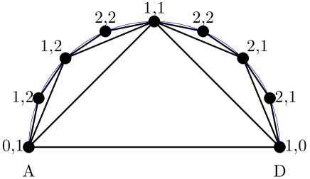
Figure 5: The first three steps of the network with $q=0$, with the nodes labeled by ordered pairs denoting the shortest distance to the left and right end nodes.

We consider a node $i\in N_{t}^{(1)}$ and the shortest-path distances to $A$ and $D$, i.e., $d_{iA}$ and $d_{iD}$. After the step $t_{i}$ when the node $i$ was generated, the values of $d_{iA}$ and $d_{iD}$ do not change at subsequent steps, since the shortest paths are always along the edges added earliest. We see this in Fig. 5, where the nodes are labeled by the ordered pairs $d_{iD},\,d_{iA}$, for the first three iterative steps. We denote by $a^{t}_{m,m^{\prime}}$ the number of nodes added at step $t$ which have $d_{iA}=m$, $d_{iD}=m^{\prime}$. Since $A$ and $D$ are connected, $m^{\prime}$ and $m$ can differ by at most 1. Thus for a given $m$ there are three categories of nodes added at step $t$, respectively numbering $a^{t}_{m,m+1},a^{t}_{m,m}$, and $a^{t}_{m+1,m}$. By symmetry $a^{t}_{m+1,m}=a^{t}_{m,m+1}$. The $m$, $m^{\prime}$ values of nodes added at step $t$ depend on the neighbor nodes, which were added at previous steps. For example, there is one node added at step $t$ ($t\geq 2$) which is a nearest-neighbor of $A$, so this new node has $m=1$, $m^{\prime}=2$, giving $a^{t}_{1,2}=1$. Nodes with $m=1$, $m^{\prime}=2$ will in turn get neighbors with $m=2$, $m^{\prime}=3$ in subsequent steps. The relationship between $a^{t}_{2,3}$ and $a^{k}_{1,2}$ for $k<t$ is

$$a^{t}_{2,3}=\sum_{k=2}^{t-2}2\,a^{k}_{1,2}=2(t-3)\,.$$ (21)

Similarly,

$$a^{t}_{3,4}=\sum_{k=4}^{t-2}2\,a^{t}_{2,3}=2(t-4)(t-5)\,.$$ (22)

Since nodes with distances $m$, $m+1$ do not appear before the step $t=2m$, the sum over $a^{k}_{2,3}$ starts at $k=4$. Proceeding in this way, for general $m\geq 1$ and $t\geq 2m$,

$$a^{t}_{m,m+1} =\sum_{k=2(m-1)}^{t-2}2\,a^{k}_{m-1,m}$$

$$=\frac{2^{m-1}(t-m-1)!}{(m-1)!(t-2m)!}\,.$$ (23)

The value of $a^{t}_{0,1}$ is $1$ for $t=0$ and $0$ for $t>0$. Analogously, for general $m\geq 2$ and $t\geq 2m-1$,

$$a^{t}_{m,m}=\frac{2^{m-1}(t-m-1)!}{(m-2)!(t-2m+1)!}\,.$$ (24)

The value of $a^{t}_{1,1}$ is $1$ for $t=1$ and $0$ for $t>1$.

As derived in the Appendix, we can obtain the quantities in Eq. (19),

$$V^{\text{near}}_{t} =\sum_{k=1}^{t}\sum_{m=0}^{\lfloor k/2\rfloor}a^{k}_{m,m+1}=\begin{cases}\frac{1}{3}2^{t}+\frac{1}{3},\ &\ t\ \text{is odd}\\ \frac{1}{3}2^{t}+\frac{2}{3},\ &\ t\ \text{is even}\end{cases}$$

$$V^{\text{mid}}_{t} =\sum_{k=1}^{t}\sum_{m=1}^{\lfloor k/2\rfloor}a^{k}_{m,m}=\begin{cases}\frac{1}{3}2^{t}+\frac{1}{3},\ &\ t\ \text{is odd}\\ \frac{1}{3}2^{t}-\frac{1}{3},\ &\ t\ \text{is even}\end{cases}$$

$$d^{\text{near}}_{t} =\sum_{k=1}^{t}\sum_{m=0}^{\lfloor k/2\rfloor}ma^{k}_{m,m+1}$$

$$=\begin{cases}-\frac{1}{27}-\frac{1}{27}2^{t}-\frac{1}{9}t+\frac{1}{9}t2^{t},\ &\ t\ \text{is odd}\\ \frac{1}{27}-\frac{1}{27}2^{t}+\frac{1}{9}t+\frac{1}{9}t2^{t},\ &\ t\ \text{is even}\end{cases}$$

$$d^{\text{mid}}_{t} =\sum_{k=1}^{t}\sum_{m=1}^{\lfloor k/2\rfloor}ma^{k}_{m,m}$$

$$=\begin{cases}\frac{5}{27}+\frac{5}{27}2^{t}+\frac{2}{9}t+\frac{1}{9}t2^{t},\ &\ t\ \text{is odd}\\ \frac{11}{27}+\frac{5}{54}2^{t}-\frac{1}{9}t+\frac{1}{18}t2^{t},\ &\ t\ \text{is even}\end{cases}$$

where $\lfloor x\rfloor$ denotes the largest integer $\leq x$ and the different results for $t$ odd and even are given consecutively, and

$$d^{\text{far}}_{t} =\sum_{k=1}^{t}\sum_{m=0}^{\lfloor k/2\rfloor}(m+1)a^{k}_{m,m+1}=d_{t}^{\text{near}}+V_{t}^{\text{near}}\,.$$ (26)

Substituting the results of Eq. (LABEL:eqapp40) into Eq. (20), we can otain

$$\Delta_{t}=\frac{1}{18}\left[-5-3(-1)^{t}+12\cdot 2^{t}+14\cdot 2^{2t}+12\,t\,4^{t}\right].$$ (27)

Substituting Eq. (27) for $\Delta_{m}$ into Eq. (18), and using $S_{1}=3$, we have

$$S_{t}=\begin{cases}\frac{3}{2}\cdot 2^{t}+\frac{1}{18}(4-5\cdot 2^{2t}-10\cdot 2^{t}+6\,t\,2^{t}\\ +6\,t\,2^{2t}),t\ \text{is odd};\\ \frac{3}{2}\cdot 2^{t}+\frac{1}{18}(6-5\cdot 2^{2t}-10\cdot 2^{t}+6\,t\,2^{t}\\ +6\,t\,2^{2t}),t\ \text{is even}.\end{cases}$$ (28)

Inserting Eq. (28) into Eq. (11), we obtain the exact expressions for average path length $\bar{d}_{t}$ which is of the form

$$\bar{d}_{t}=\begin{cases}\frac{17+2^{2-t}-5\cdot 2^{t}+6t(1+2^{t})}{9(1+2^{t})},&\ t\ \text{is odd};\\ \frac{17+3\cdot 2^{1-t}-5\cdot 2^{t}+6t(1+2^{t})}{9(1+2^{t})},\ &\ t\ \text{is even}.\end{cases}$$ (29)

In the infinite network size limit ($t\rightarrow\infty$),

$$\bar{d}_{t}\simeq\frac{2}{3}t-\frac{5}{9}\simeq\ln V_{t}-\frac{5}{9}.$$ (30)

Thus, the average path length logarithmically grows with increasing size of the network. This logarithmic scaling of $\bar{d}_{t}$ with network size, together with the large clustering coefficient obtained in the preceding section, shows that in the case of $q=0$ the graph is a small-world network.

3.3.3 Case of $0<q<1$

For $0<q<1$, in order to obtain the variation of the average path length with the parameter $q$, we have performed extensive numerical simulations for different $q$ between 0 and 1. Simulations were performed for network $N_{15}$ with size $16385$, averaging over 20 network samples for each value of $q$. In Fig. 6, we plot the average path length as a function of $q$. We observe that, when lessening $q$ from 1 to 0, average path length drops drastically from a very high value a small one, which predicts that a phase transition from large-world to small-world occurs. This behavior is similar to that in the WS model.

Figure 6: Graph of the dependence of an average path length on the tunable parameter $q$.

Why is the average path length low for small $q$? The explanation is as follows. The older nodes that had once been nearest neighbors along the semi-ring are pushed apart as new nodes are positioned in the interval between them. From Fig. 1 we can see that when new nodes enter into the networks, the original nodes are not near but, rather, have many newer nodes inserted between them. When $q$ is small, the network growth creates enough ”shortcuts” (i.e. long-range edges) attached to old nodes, which join remote nodes along the semi-ring one another as in the WS model [6]. These shortcuts drastically reduces the average path length, leading to a small-world behavior.

4 Conclusions

In summary, we have presented and studied a one-parameter model of the time evolution of geometrically growing networks. In our model, in addition to the widely considered case of addition of new nodes and new edges which connect new nodes and old ones, we also consider edge (linking old nodes) removal. The presented model interpolates between one-dimensional regular chains and small-world networks, which allow us to explore the crossover between the two limiting cases. We have obtained the analytical and numerical results for degree distribution and clustering coefficient, as well as the average path length, which are determined by the model parameter $q$. The observed topological behaviors are similar to those in the WS model.

Our model may provide a useful tool to investigate the influence of the clustering coefficient or average path length in different dynamics processes taking place on networks. In addition, using the idea presented here, we can also establish a scale-free network model which undergoes two interesting phase transitions: from a large world to a small world, and from a fractal topology to a non-fractal structure. The details will be published elsewhere.

Appendix A Derivations of $V_{t}^{\text{near}}$ and $d_{t}^{\text{near}}$

In this Appendix, we give the computation details of $V_{t}^{\text{near}}$ and $d_{t}^{\text{near}}$, respectively. Other quantities in Eq. (19) can be derived analogously. Here we only address the case of even $t=2T$ ($T$ is positive integer). For odd $t$, we can proceed in the same way.

First, we compute $V_{t}^{\text{near}}$. We rewrite $a_{m,m+1}^{t}$ and $a_{m,m}^{t}$ as

$$\begin{cases}a_{m,m+1}^{t}=2^{m-1}C_{t-m-1}^{m-1},&\ 2m\leq t;\\ a_{m,m}^{t}=2^{m-2}C_{t-m-1}^{m-2},&\ 2m\leq t+1.\end{cases}$$ (31)

For even $t=2T$, we have

$$V_{t}^{\text{near}} = \sum_{k=1}^{t}\sum_{2m\leq k}a_{m,m+1}^{k}(m\geq 1)+1(A\ \text{itself})$$ (32)

$$= \sum_{m=1}^{T}\sum_{k=2m}^{2T}a_{m,m+1}^{k}+1$$

$$= \sum_{m=1}^{T}\sum_{k=2m}^{2T}2^{m-1}C_{k-m-1}^{m-1}+1$$

$$= \sum_{m=1}^{T}2^{m-1}\sum_{k=2m}^{2T}C_{k-m-1}^{m-1}+1.$$

To find $\sum_{k=2m}^{2T}C_{k-m-1}^{m-1}$, we use the approach based on generating functions [24]. We define

$$G_{1}(x)=\sum_{k=2m}^{2T}(1+x)^{k-m-1},$$ (33)

and denote by $z$ the coefficient of power of $x^{m-1}$ in $G_{1}(x)$. Then, we have $z=\sum_{k=2m}^{2T}C_{k-m-1}^{m-1}$. At the same time, we can sum the items in right hand of Eq. (33) and obtain $G_{1}(x)$ as

$$G_{1}(x) = \frac{1-(1+x)^{2T-2m+1}}{1-(1+x)}(1+x)^{m-1}$$ (34)

$$= \frac{(1+x)^{2T-m}-(1+x)^{m-1}}{x}.$$

From Eq. (34), it is obvious that the coefficient of power of $x^{m-1}$ in $G_{1}(x)$ is $C_{2T-m}^{m}$, thus $z=\sum_{k=2m}^{2T}C_{k-m-1}^{m-1}=C_{2T-m}^{m}$. Then Eq. (32) can be written as

$$V_{t}^{\text{near}}=\sum_{m-1}^{T}2^{m-1}C_{2T-m}^{m}+1.$$ (35)

All that is left to obtain $V_{t}^{\text{near}}$ is to evaluate the sum in Eq. (35), which is denoted as $u$. In order to find $u$, we define

$$G_{2}(x)=\sum_{m=1}^{T}2^{m-1}(1+x)^{2T-m}x^{T-m}.$$ (36)

Then $u$ exactly equals the coefficient of the power of $x^{T}$ in $G_{2}(x)$. By summing over all $m$, we get $G_{2}(x)$ as

$$G_{2}(x) = \frac{2^{T}(1+x)^{T}-x^{T}(1+x)^{2T}}{(1-x)(x+2)}$$ (37)

$$= \frac{1}{3}\left(\frac{1}{1-x}+\frac{1}{x+2}\right)$$

$$\left[2^{T}(1+x)^{T}-x^{T}(1+x)^{2T}\right].$$

And since

$$\frac{1}{1-x}=1+x+x^{2}+\cdots=\sum_{t=0}^{\infty}x^{t}$$

and

$$\frac{1}{x+2}=\frac{1}{2}\sum_{t=0}^{\infty}\left(-\frac{1}{2}x\right)^{t},$$

we have $u=\frac{1}{3}2^{2T}-\frac{1}{3}$. Hence

$$V_{t}^{\text{near}}=u+1=\frac{1}{3}2^{t}+\frac{2}{3}$$ (38)

as shown in Eq. (LABEL:eqapp40).

Next, we compute $d_{t}^{\text{near}}$ based on a similar derivation process of $V_{t}^{\text{near}}$. We rewrite $d_{t}^{\text{near}}$ in the form

$$d_{t}^{\text{near}} = \sum_{k=1}^{t}\sum_{2m\leq k}ma_{m,m+1}^{k}\ (m\geq 1)$$ (39)

$$= \sum_{m=1}^{T}m2^{m-1}C_{2T-m}^{m}.$$

After above simplification, what is left is to find the sum over all $m$, which we denote as $Q_{T}$. Then

$$Q_{T} = \sum_{m=1}^{T}m2^{m-1}C_{2T-m}^{m}$$ (40)

$$= \sum_{m=1}^{T}2^{m-1}(2T-m)C_{2T-m-1}^{m-1}$$

$$= \sum_{m=1}^{T}2^{m-1}(2T-1)C_{2T-m-1}^{m-1}$$

$$-\sum_{m=1}^{T}2^{m-1}(m-1)C_{2T-m-1}^{m-1}$$

$$= \frac{1}{3}(2T-1)\left(2^{2T-1}+1\right)-2Q_{T-1}.$$

Making using of $Q_{1}=1$, Eq. (40) can be solved inductively,

$$Q_{T} = (-2)^{T-1}Q_{1}$$ (41)

$$+\sum_{m=1}^{T-1}(-2)^{T-m-1}\frac{1}{3}(2m+1)\left(2^{2m+1}+1\right)$$

$$= \frac{1}{27}-\frac{1}{27}4^{T}+\frac{2}{9}\,T+\frac{2}{9}\,T\,4^{T},$$

as given in Eq. (LABEL:eqapp40).

References

• [1] M. E. J. Newman, Models of the small world, Journal of Statistical Physics, 101 (2000), 819-841.
• [2] R. Albert and A.-L. Barabási, Statistical mechanics of complex networks, Reviews of Modern Physics, 74(1) (2002), 47-97.
• [3] S. N. Dorogvtsev and J. F. F. Mendes, Evolution of networks, Advances in Physics, 51(4) (2002), 1079-1187.
• [4] M. E. J. Newman, The structure and function of complex networks, SIAM Review, 45(2) (2003), 167-256.
• [5] S. Boccaletti, V. Latora, Y. Moreno, M. Chavez and D.-U. Hwanga, Complex networks: Structure and dynamics, Physics Reports, 424 (2006), 175-308.
• [6] D. J. Watts and S. H. Strogatz, Collective dynamics of small-world networks, Nature, 393 (1998), 440-442.
• [7] M. Barthélémy and L. A. N. Amaral, Small-World networks: Evidence for a crossover picture, Physical Review Letters, 82 (1999), 3180-3183.
• [8] M. E. J. Newman and D. J. Watts, Renormalization group analysis of the small-world network model, Physics Letters A, 263 (1999), 341-346.
• [9] A. Barrat, and M. Weigt, On the properties of small-world network, The European Physical Journal B, 13 (2000), 547-560.
• [10] J. Kleinberg, Navigation in a small world, Nature, 406 (2000), 845-845.
• [11] F. Comellas, J. Ozón, and J.G. Peters, Deterministic small-world communication networks, Information Processing Letters, 76 (2000), 83-90.
• [12] J. Ozik, B.-R. Hunt, and E. Ott, Growing networks with geographical attachment preference: Emergence of small worlds, Physical Review E, 69 (2004), 026108.
• [13] Z. Z. Zhang, L. L. Rong, and C. H. Guo, A deterministic small-world network created by edge iterations, Physica A, 363 (2006), 567-572.
• [14] Z. Z. Zhang, L. L. Rong, and F. Comellas, Evolving small-world networks with geographical attachment preference, Journal of Physics A, 39 (2006), 3253-3261.
• [15] A.-L. Barabási and R. Albert, Emergence of scaling in random networks, Science 286 (1999), 509-512.
• [16] R. Albert, and A.-L. Barabási, Topology of evolving networks: Local events and universality, Physical Review Letters, 85 (2000), 5234-5237.
• [17] S. N. Dorogovtsev, and J. F. F. Mendes, Scaling behaviour of developing and decaying networks, Europhysics Letters 52(1) (2000), 33-39.
• [18] C. Moore, G. Ghoshal, and M. E. J. Newman, Exact solutions for models of evolving networks with addition and deletion of nodes, Physical Review E, 74 (2006), 036121.
• [19] W.-X. Wang, B.-H. Wang, B. Hu, G. Yan, and Q. Ou, General dynamics of topology and traffic on weighted technological networks, Physical Review Letters, 94 (2005), 188702.
• [20] D. H. Shi, L. M. Liu, X. Zhu, and H. J. Zhou, Degree distributions of evolving networks, Europhysics Letters, 76(4) (2006), 10315.
• [21] S. N. Dorogovtsev, A. V. Goltsev, and J. F. F. Mendes, Pseudofractal scale-free web, Physical Review E, 65 (2002), 066122.
• [22] E. Ravasz and A.-L. Barabási, Hierarchical organization in complex networks, Physical Review E, 67 (2003), 026112.
• [23] M. Hinczewski and A. N. Berker, Inverted Berezinskii-Kosterlitz-Thouless singularity and high-temperature algebraic order in an Ising model on a scale-free hierarchical-lattice small-world network, Physical Review E, 73 (2006), 066126.
• [24] M. E. J. Newman, S. H. Strogatz, and D. J. Watts, Random graphs with arbitrary degree distributions and their application, Physical Review E, 64 (2001), 026118.