Random matrix analysis of complex networks

Abstract

We study complex networks under random matrix theory (RMT) framework. Using nearest-neighbor and next-nearest-neighbor spacing distributions we analyze the eigenvalues of adjacency matrix of various model networks, namely, random, scale-free and small-world networks. These distributions follow Gaussian orthogonal ensemble statistic of RMT. To probe long-range correlations in the eigenvalues we study spectral rigidity via $\Delta_{3}$ statistic of RMT as well. It follows RMT prediction of linear behavior in semi-logarithmic scale with slope being $\sim 1/\pi^{2}$. Random and scale-free networks follow RMT prediction for very large scale. Small-world network follows it for sufficiently large scale, but much less than the random and scale-free networks.

I Introduction

Random matrix theory (RMT), initially proposed to explain statistical properties of nuclear spectra, had successful predictions for the spectral properties of different complex systems such as disordered systems, quantum chaotic systems, large complex atoms, etc., followed by numerical and experimental verifications in the last few decades mehta ; rev-rmt . Quantum graphs, which model the systems of interest in quantum chemistry, solid state physics and transmission of waves, have also been studied under the RMT framework Qgraph . Recently, RMT has been shown to be useful also in understanding the statistical properties of empirical cross-correlation matrices appearing in the study of multivariate time series of followings: price fluctuations in stock market rmt-stock1 ; rmt-stock2 , EEG data of brain rmt-brain , variation of different atmospheric parameters rmt-atmosphere , etc.

In our previous studies pap1 ; pap2 complex networks have been analyzed under RMT framework. These works consider nearest-neighbor spacing distribution (NNSD) of eigenvalues spectra of adjacency and Laplacian matrices of various extensively studied networks. The NNSD gives probability for finding neighboring eigenvalues with a given spacing, and it follows two universal properties depending upon underlying correlations among the eigenvalues. For the correlated eigenvalues, NNSD follows Gaussian orthogonal ensemble (GOE) statistics of RMT, whereas it follows Poissonian statistics for the uncorrelated eigenvalues. One of the main advantages of RMT approach is that depending on the nature of eigenvalues correlations one can separate system dependent part from random universal part, which are intermingled due to the complexity of the system rev-rmt ; rmt-stock1 ; rmt-stock2 ; rmt-brain ; rmt-atmosphere . RMT analysis for the various networks shows that the NNSD of complex networks also follow universal GOE statistics of RMT pap1 . This finding suggests that different results of GOE statistics, which have successfully been applied to understand the systems coming from various fields starting from nuclei to the stock-market, can be applied to study networks as well. Our earlier works concentrate on the NNSD studies of networks. NNSD carries information for the correlation between two adjacent eigenvalues, but do not tell about the correlation between two far-off eigenvalues. Therefore, even though NNSD follows GOE statistics of RMT, other properties may show deviations, which suggests that one can not rely on NNSD results exclusively. To probe for long-range correlations as well, current work considers spectral rigidity test via well known $\Delta_{3}$-statistic of RMT. It is found that the spectral rigidity of the complex networks follows RMT prediction, with scale depending upon the properties of the networks. Present work also analyzes the next-nearest-neighbor spacing distribution (nNNSD) of the adjacency matrix of the networks.

The paper is organized as follows: following the above introduction, Sec. II explains various aspects of complex networks studies. Sec. III describes some basics of RMT relevant to our studies. Sec. IV illustrates the RMT analysis for various model networks, namely; random, scale-free and small world. The NNSD is the most widely studied property in random matrix literature, therefore, this section includes NNSD results for the above mentioned model networks pap1 , and presents results for nNNSD and the $\Delta_{3}$-statistic of these networks. Finally, Sec. V discusses and summarizes results with some possible future directions.

II Complex networks

Last 10 years have witnessed a rapid advancement in the studies of complex networks. The main concept of the network theory is to define complex systems in terms of networks of many interacting units. Few examples of such systems are interacting molecules in living cell, nerve cells in brain, computers in Internet communication, social networks of interacting people, airport networks with flight connections, etc rev-Strogatz ; rev-network ; rev-Boccaletti . In the graph theoretical terminology, units are called nodes and interactions are called edges graph . Various model networks have been introduced to study the behavior of complex systems having underlying network structures. These model networks are based on simple principles, still they capture essential features of the underlying systems.

II.1 Structural properties

In random graph model of Erdös and Rényi any two nodes are randomly connected with probability $p$ erdos . This model assumes that interactions between nodes are random. Recently, with the availability of large maps of real world networks, it has been observed that the random graph model is not appropriate for studying the behavior of real world networks. Hence many new models have been introduced. Watts and Strogatz proposed a model, popularly known as ‘small-world network’, which has properties of small diameter and high clustering SW . Moreover, this model network is very sparse : network with a very few number of edges, another property shown by many real-world networks. In addition to the above mentioned properties, Barabási and Albert show that degree distributions of many real-world networks have power-law. This implies that some nodes are much more connected than the others BA . Barabási-Albert’s scale-free model and Watts-Strogatz’s small-world model have contributed immensely in understanding evolution and behavior of the real systems having network structures. Following these two new models came an outbreak in the field of networks. These studies show that real world networks have coexistence of randomness and regularity rev-Strogatz ; Newman ; rev-Costa .

II.2 Spectral properties

Apart from the above mentioned investigations which focus on direct measurements of the structural properties of networks, there have been lot of studies demonstrating that properties of networks or graphs could be well characterized by the spectrum of associated adjacency matrix $A$ spectrum . For an unweighted graph, it is defined in the following way : $A_{ij}=1$, if $i$ and $j$ nodes are connected and $zero$ otherwise. For an undirected network, this matrix is symmetric and consequently has real eigenvalues. Eigenvalues give information about some basic topological properties of the underlying network spectrum ; handbook . Spectral properties of networks have also been used to understand some of the dynamical properties of interacting chaotic units on networks, for example largest eigenvalue of adjacency matrix determines transition to the synchronized state ott . The distribution of the eigenvalues of a matrix having finite probability $p$ of nonzero Gaussian distributed random elements per row, follows Wigner semicircular law in the limit $p\rightarrow 1$. For very small $p$ also, which corresponds to the sparse random matrix, one gets semicircular law with several peaks at different eigenvalues sparseRM .

With the increasing availability of large maps of real-world networks, analyses of spectral densities of adjacency matrix of real-world networks and model networks having real-world properties have also begun Vicsek ; Dorogovtsev ; Kim ; Aguiar . These analyses show that the matrix constructed by $zero$ and $one$ elements corresponding to a unweighted random network, also follows Wigner semicircular law Vicsek with degeneracy at $\lambda=0$. Small-world model networks show very complex spectral density with many sharp peaks Aguiar , while the spectral density of scale-free model networks exhibits so called triangular distribution Vicsek ; Kim ; Aguiar . Spectral density and NNSD of the random matrices constructed by $zero$ and $one$ elements have been studied extensively in the Ref. bauer . These studies show that NNSD of the random matrices follow GOE distribution of RMT.

III Random matrix statistics

In the random matrix studies of eigenvalues spectra, one has to consider two kinds of properties : (1) global properties, like spectral density or distribution of eigenvalues $\rho(\lambda)$, and (2) local properties, like eigenvalue fluctuations around $\rho(\lambda)$. Among these, the eigenvalue fluctuations is the most popular one. This is generally obtained from the NNSD of the eigenvalues. The eigenvalues of network are denoted by $\lambda_{i},\,\,i=1,\dots,N$, where $N$ is the size of the network and $\lambda_{i}<\lambda_{i+1},\,\,\forall i$. In order to get universal properties of the eigenvalue fluctuations, one has to remove the spurious effects due to the variations of spectral density and to work at constant spectral density on the average. Thereby, it is customary in RMT to unfold the eigenvalues by a transformation $\overline{\lambda}_{i}=\overline{N}(\lambda_{i})$, where $\overline{N}(\lambda)=\int_{\lambda_{\mbox{\tiny min}}}^{\lambda}\,\rho(\lambda^{\prime})\,d\lambda^{\prime}$ is the averaged integrated eigenvalue density mehta . Since analytical form for $\overline{N}$ is not known, we numerically unfold the spectrum by polynomial curve fitting. Using the unfolded spectrum, we calculate the nearest-neighbor spacings as

$$s_{1}^{(i)}=\overline{\lambda}_{i+1}-\overline{\lambda}_{i};$$

and due to the above unfolding, the average nearest-neighbor spacings $\langle s_{1}\rangle$ becomes unity, being independent of the system. The NNSD $P(s_{1})$ is defined as the probability distribution of these $s_{1}^{(i)}$’s. In case of Poisson statistics,

$$P(s_{1})=\exp(-s_{1});$$ (1)

whereas for GOE

$$P(s_{1})=\frac{\pi}{2}s_{1}\exp\left(-\frac{\pi s_{1}^{2}}{4}\right).$$ (2)

For the intermediate cases, NNSD is described by Brody formula brody :

$$P_{\beta}(s_{1})=As_{1}^{\beta}\exp\left(-Bs_{1}^{\beta+1}\right),$$ (3a)

where $$A B \beta$$ and are determined by the parameter as follow :

$$A\,=\,(1+\beta)\alpha\,\mbox{and}\,\alpha=\left[\Gamma\left(\frac{\beta+2}{\beta+1}\right)\right]^{\beta+1}.$$ (3b)

This is a semiempirical formula characterized by the single parameter $\beta$, popularly known as Brody parameter. $\beta=1$ corresponds to the GOE statistics and $\beta=0$ corresponds to the Poisson statistics.

Apart from NNSD, the next-nearest-neighbor spacings distribution (nNNSD) is also used to characterize the statistics of eigenvalues fluctuations. We calculate this distribution $P(s_{2})$ of next-nearest-neighbor spacings

$$s_{2}^{(i)}=(\overline{\lambda}_{i+2}-\overline{\lambda}_{i})/2$$ (4)

between the unfolded eigenvalues. Factor of two at the denominator is inserted to make the average of next-nearest-neighbor spacings $\langle s_{2}\rangle$ unity. According to Ref. mehta , the nNNSD of GOE matrices is identical to the NNSD of Gaussian symplectic ensemble (GSE) matrices, i.e.,

$$P(s_{2})=\frac{2^{18}}{3^{6}\pi^{3}}\,s_{2}^{4}\exp\left(-\frac{64}{9\pi}\,s_{2}^{2}\right).$$ (5)

The NNSD and nNNSD reflect only local correlations among the eigenvalues. The spectral rigidity, measured by the $\Delta_{3}$-statistic of RMT, gives information about the long-range correlations among eigenvalues and is more sensitive test for RMT properties of the matrix under investigation mehta ; casati . In the following we describe the procedure to calculate this quantity.

The $\Delta_{3}$-statistic measures the least-square deviation of the spectral staircase function representing the averaged integrated eigenvalue density $\overline{N}(\lambda)$ from the best straight line fitting for a finite interval $L$ of the spectrum, i.e.,

$$\Delta_{3}(L;x)=\frac{1}{L}\min_{a,b}\int_{x}^{x+L}\,\left[N(\overline{\lambda})-a\overline{\lambda}-b\right]^{2}\,d\overline{\lambda}$$ (6)

where $a$ and $b$ are obtained from a least-square fit. Average over several choices of $x$ gives the spectral rigidity $\Delta_{3}(L)$. For the Poisson case, when the eigenvalues are uncorrelated, $\Delta_{3}(L)=L/15$, reflecting strong fluctuations around the spectral density $\rho(\lambda)$. On the other hand, for the GOE case, $\Delta_{3}(L)$ depends logarithmically on $L$, i.e.,

$$\Delta_{3}(L)\sim\frac{1}{\pi^{2}}\ln L.$$ (7)

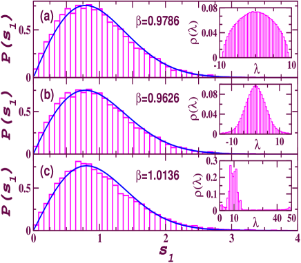
Figure 1: (Color online) Nearest-neighbor spacings distribution (NNSD) $P(s_{1})$ of the adjacency matrices of different networks [(a) random network, (b) scale-free network, and (c) small-world network]. All follow GOE statistics. The histograms are numerical results and the solid lines represent fitted Brody distribution (Eq.(3)). All networks have $N=2000$ nodes and an average degree $k=20$ per node. Figures are plotted for average over 10 random realizations of the networks. Insets show respective spectral densities $\rho(\lambda)$.

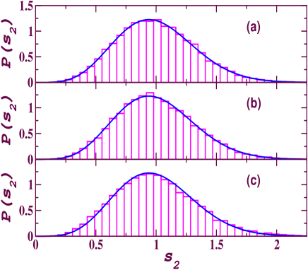
Figure 2: (Color online) Next-nearest-neighbor spacings distribution (nNNSD) $P(s_{2})$ of the adjacency matrices of different networks [(a) random network, (b) scale-free network, and (c) small-world network] is compared with the nearest-neighbor spacings distribution (NNSD) of GSE matrices. Figures are plotted for average over 10 realization of the networks. All networks have $N=2000$ nodes and an average degree $k=20$ per node.

IV Results

In the following we present results for the ensemble averaged NNSD, nNNSD and $\Delta_{3}$ statistic of random, scale-free and small-world networks.

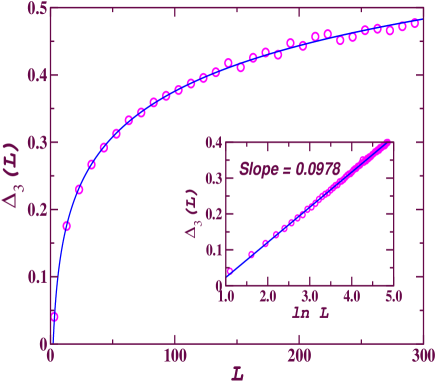
Figure 3: (Color online) $\Delta_{3}(L)$ statistic for eigenvalues spectra of the random network. The circles are numerical results and the solid curve is GOE prediction of RMT. Inset shows the $\Delta_{3}(L)$ in semi-logarithmic scale, in this scale it has the slope $0.0978$. Figure is plotted for average over 10 realizations of the networks. All networks have $N=2000$ nodes and an average degree $k=20$ per node.

IV.1 Random network

First we consider an ensemble of random networks generated by using Erdös-Rényi algorithm. Starting with $N=2000$ nodes random connections between pairs of nodes are made with probability $p$. The average degree of the graph is $k=2n/N=p(N-1)\sim pN$. There exists a critical probability $p_{c}(N)$ for which one gets a large connected component. The degree distribution of this random graph is a binomial distribution $P(k)=C^{k}_{N-1}p^{k}(1-p)^{N-1-k}$. For $p=0.01$, this method yields a connected network with average degree $p\times N=20$. Note that for very small value of $p$ one gets several disconnected components. In this study choice of $p$ is high enough to give a connected component typically spanning all the nodes.

We calculate the eigenvalues spectrum of network generated according to the above algorithm. First the eigenvalues are unfolded by using the technique described in Sec. III. This method yields the eigenvalues with constant spectral density on the average. These unfolded eigenvalues are used to calculate NNSD. The same procedure is repeated for an ensemble of the networks generated for different random realizations. Note that $p$ is always chosen such that algorithm generates a network with average degree $k=20$. Fig.1(a) plots ensemble average of NNSD. By fitting this ensemble averaged NNSD with the Brody formula given in Eq.(3) we get an estimation of the Brody parameter $\beta=0.9786\sim 1$. This value of Brody parameter clearly indicates the GOE behavior of the NNSD [Eq. (2)]. Inset of Fig. 1(a) shows corresponding spectral density which follows well known Wigner’s semicircular distribution. The same unfolded eigenvalues are used to calculate nNNSD. For this we calculate next nearest neighbor spacings as given in Eq. (4) and plot their distribution in Fig. 2(a). It can be seen from the figure that the nNNSD agrees well with the NNSD of GSE matrices as given in Eq. (5).

As explained in the introduction that NNSD and nNNSD only tell about the short range correlations among the eigenvalues. Therefore, to probe for the long range correlations we study $\Delta_{3}(L)$ statistic of the spectrum of this network. $\Delta_{3}(L)$ is calculated following Eq. (6). Fig. 3 plots this statistics for the same ensemble as used for the NNSD and nNNSD calculations above. It can be seen that $\Delta_{3}(L)$ statistic agrees very well with the RMT prediction, given by Eq. (7), upto very large value of $L$, i.e., $L\sim 300$. Inset of this figure shows the same in semi-logarithmic scale. Here one can see the expected linear behavior of $\Delta_{3}(L)$ with slope of $0.0978$ which is very close to the RMT predicted value $1/\pi^{2}\sim 0.1013$ [Eq.(7)].

Note that here an ensemble of ten networks of dimension $N=2000$ is considered. Statistical properties of eigenvalues spectra of members of this ensemble have very small deviations from each other and hence justifying ensemble averaging calculations ergodicity-RMT . Each individual network in the ensemble follows random matrix predictions with very good accuracy, however to make the statistical analysis more credible, we present the results for an ensemble of ten networks. Here we would like to mention that an ensemble of networks of much smaller dimensions, say $N=100$, has been studied as well and it follows GOE predictions of RMT. However, for this case, many more realizations are required to get good accuracy.

IV.2 Scale-free network

Scale-free network is generated by using the model of Barabási and Albert BA . Starting with a small number, $m_{0}$ of the nodes, a new node with $m\leq m_{0}$ connections is added at each time step. This new node connects with an already existing node $i$ with probability $\pi(k_{i})\propto k_{i}$, where $k_{i}$ is the degree of the node $i$. After $\tau$ time steps the model leads to a network with $N=\tau+m_{0}$ nodes and $m\tau$ connections. This model generates a scale-free network, i.e., the probability $P(k)$, that a node has degree $k$ decays as a power law $P(k)\sim k^{-\lambda}$, where $\lambda$ is a constant and for the type of probability law $\pi(k)$ used here $\lambda=3$. Other forms for the probability $\pi(k)$ are also possible which give different values of $\lambda$. However, the results reported here are independent of the value of $\lambda$.

Using the above algorithm an ensemble of scale-free networks of size $N=2000$ and average degree $k=20$ is generated. To calculate NNSD, nNNSD and $\Delta_{3}$ for the spectra of this ensemble, we follow the same procedure as described in the previous section. Fig. 1(b) shows that the NNSD of scale-free network follows GOE with $\beta=0.9626\sim 1$. Inset of this figure plots the spectral density of this network. Fig. 2(b) shows that the nNNSD of the adjacency matrix of this network agrees well with the NNSD of the GSE matrices. Fig. 4 shows the $\Delta_{3}(L)$ statistic for the adjacency matrix of scale-free network. Here we see that the $\Delta_{3}(L)$ statistic for the scale-free network agrees very well with the RMT prediction for very large $L$, i.e., $L\sim 150$, and deviations are seen only after $L=150$. Inset of this figure shows the expected linear behavior of $\Delta_{3}(L)$ in semi-logarithmic scale for $L\lesssim 150$ with the slope of $0.0975$, a value very close to the RMT predicted value $1/\pi^{2}$.

Universality of NNSD and nNNSD for random and scale-free networks seems to give the impression that these networks have same amount of randomness but $\Delta_{3}$ results tell that the scale-free network is not as much random as the random network. This is obvious from their construction algorithms as well, but $\Delta_{3}$ statistics is capturing this property which is a very important result. The finding also suggests that scale-free networks have some specific features that cannot be modeled by RMT. It may be noted that one can generate scale-free networks by using other algorithms as well kim ; mendes , for these networks also spacing distributions and spectral rigidity results will have qualitatively similar behaviors, except that the range of agreement of $L$ with the random matrix prediction would depend upon the amount of randomness in the networks.

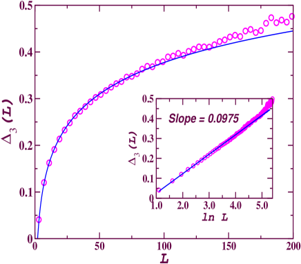
Figure 4: (Color online) $\Delta_{3}(L)$ statistic for eigenvalues spectra of the scale-free network. The circles are numerical results and the solid curve is the GOE prediction of RMT. Inset plots the $\Delta_{3}(L)$ in semi-logarithmic scale, in this scale it has the slope $0.0975$. Figure is plotted for the average over 10 realizations of the networks. All networks have $N=2000$ nodes and an average degree $k=20$ per node.

IV.3 Small-world network

Small-world networks are constructed using the following algorithm of Watts and Strogatz SW . Starting with an one-dimensional ring lattice of $N$ nodes in which every node is connected to its $k/2$ nearest neighbors, we randomly rewire each connection of the lattice with the probability $p$ such that self-connections and multiple connections are excluded. Thus $p=0$ gives a regular network and $p=1$ gives a completely random network. The typical small-world behavior is observed around $p=0.005$ pap1 . For $N=2000$ and average degree $k=20$, an ensemble of ten different realizations of the network are generated.

Again the same procedure as described in Sec. IV.1 has been used to calculate NNSD, nNNSD and $\Delta_{3}$ for the spectra. Fig.1(c) shows that the NNSD of this network again follows GOE statistics with $\beta$ very close to $1$, i.e., $\beta=1.0136$. The inset shows that the corresponding spectral density is complicated with several peaks. One peak is always at $\lambda=0$. The exact positions of other peaks may vary but overall form of spectral density remains similar. Fig. 2(c) plots the nNNSD of adjacency matrix of small-world network. It can be seen that the nNNSD agrees well with the NNSD of GSE matrices. Fig. 5 shows the $\Delta_{3}(L)$ statistic for the spectrum of adjacency matrix corresponding to the small-world network with $p=0.005$. Inset of this figure shows the expected linear behavior of $\Delta_{3}(L)$ in semi-logarithmic scale for $L\lesssim 30$ with slope of $0.1024$, a value very close to the RMT predicted value $1/\pi^{2}$. It can be seen here that $\Delta_{3}(L)$ statistics for the small-world network agrees very well with the RMT prediction for sufficiently large $L$, i.e., $L\sim 30$, but much less than the same for random and scale-free networks, implying that besides randomness, small-world network has specific features also. This again suggests that the behavior of $\Delta_{3}$ statistics can be used to understand the amount of randomness in the networks. More specifically deviation from the GOE predicted behavior corresponds to the system specific features in the network.

Note that in this paper, results for networks with the average degree 20 are presented. We have studied sparser ($\langle k\rangle<20$) and denser networks ($\langle k\rangle>20$ to $\langle k\rangle\sim N$) as well. Same universal behavior are found for these networks as far as there exists a certain amount of randomness, i.e., presence of some minimal random connections among the nodes. There exists problems with very sparse networks as of average degree two and very dense networks as of degree $\sim N$. For sparse networks ($\langle k\rangle\sim 2$) sometimes one can get several degeneracies in eigenvalues sparseRM . In this case, one has to first get rid of the degeneracies to conclude anything under the RMT framework note .

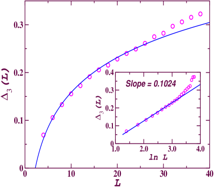
Figure 5: (Color online) $\Delta_{3}(L)$ statistic for the eigenvalues spectra of the small-world network. The circles are numerical results and the solid curve is GOE prediction of RMT. Inset plots the $\Delta_{3}(L)$ upto $L=30$ in semi-logarithmic scale, in this scale $\Delta_{3}(L)$ has the slope $0.1024$. Figure is plotted for the average over 10 realizations of the networks. All networks have $N=2000$ nodes and an average degree $k=20$ per node.

Similarly, for dense networks, universal spacing distribution are observed till very large value of average degree. For $\langle k\rangle\sim N$, largest eigenvalue has very high value than the rest of $N-1$ eigenvalues which are very close to each other, becoming equal in the limiting case of all to all connections $\langle k\rangle=N-1$. For example, random networks with $p=0.95$ (which means that the network has $95\%$ of maximum possible connections), also follow RMT predictions of universal spacing distributions till very large scale. As the number of connections are increased further one starts getting degenerate eigenvalues and for $p=0.999$ high degeneracies at various values (such as $\lambda=-1,0,1$) are observed keeping it trivially out from the RMT studies.

V Discussions

We use RMT to study complex networks and show that in spite of spectral densities of the adjacency matrices being different for different networks, their eigenvalue fluctuations are same and follow the GOE statistics of RMT. We attribute this universality to the existence of minimal amount of randomness in all these networks and show that randomness in the network connections can be quantified by the Brody parameter. In addition to the NNSD, we present the results of nNNSD and spectral rigidity via $\Delta_{3}$-statistic of RMT. The nNNSD of the eigenvalues of these model networks are identical to the NNSD of GSE matrices which again agrees with RMT prediction given in Eq. (5). NNSD and nNNSD suggest that there exists short range correlations among the eigenvalues. Spectral rigidity test shows that the $\Delta_{3}(L)$ statistics follows random matrix predicted linear behavior in semi-logarithmic plot for sufficiently large scale $L$ with slope being $\sim 1/\pi^{2}$ [see, Eq.(7)], suggesting long-range correlations among the eigenvalues. Above findings show that statistics of the bulk of eigenvalues of the model networks is consistent with those of a real symmetric random matrix and deviation from this could be understood as a system dependent part.

Universal GOE behavior of NNSD and nNNSD tell that the networks are sufficiently random, or there exists minimal amount of randomness required to introduce the correlations among the neighboring eigenvalues. The $\Delta_{3}$ analysis seems to characterize the level of randomness in networks depending on the range of correlations among eigenvalues. $\Delta_{3}$ analysis of the random network follows RMT prediction for very long range of $L$, which is not very surprising as random network follows RMT at each level starting from semi-circular density distributions. However interestingly scale-free and small-world networks also follow RMT for sufficiently large value of $L$. Beyond this value of $L$, deviation in the spectral rigidity is seen, indicating a possible breakdown of the universality. This is quite understandable as small-world network is highly clustered and scale-free network also has specific features like hubs, so it is natural that they are not as random as the random network. But it is interesting to realize that $\Delta_{3}$ statistics rightly captures this information. Moreover, small-world network is generated exactly at small-world transition by using Watts and Strogatz algorithm which yields network with very high clustering coefficient and very less number of random connections. Results presented in this paper show that these very small number of random connections make network sufficiently random to introduce the correlations among the eigenvalues for the sufficiently long range.

According to the many recent studies, randomness in connections is one of the most important and desirable ingredients for the proper functionality or the efficient performance of systems having underlying network structures. For instance, information processing in brain is considered to be because of random connections among different modular structures face . We feel that the role of random connections, and behavior and evolution of such systems can be studied better under the RMT framework. Also this RMT approach may be used to detect the connections most responsible to increase the complexity of networks. For example effect of oxygen molecule on biochemical network of a metabolic system is recently studied and is shown to increase the complexity of the system leading to a major transition in the history of life oxygen-complex .

In summary, we use RMT to analyze spectra of complex networks and show that these networks follow universal GOE statistics. These results tell that random matrix theory, a very well developed branch of Physics, can be applied to the complex networks studies. So far we have only concentrated on the model networks studied vastly in the recent literature, providing a basis to the random matrix analysis of networks. Future investigations would involve studies of real-world networks EV .

- (1) M. L. Mehta, Random Matrices, 3rd ed. (Elsevier Academic Press, Amsterdam, 2004).
- (2) T. Guhr, A. Müller-Groeling and H. A. Weidenmüller, Phys. Rep. 299, 189 (1998).
- (3) T. Kottos and U. Smilansky, Phys. Rev. Lett. 79, 4794 (1997); J. Phys. A: Math. Gen. 36, 3501 (2003).
- (4) L. Laloux, P. Cizeau, J.-P. Bouchaud, and M. Potters, Phys. Rev. Lett. 83, 1467 (1999).
- (5) V. Plerou, P. Gopikrishnan, B. Rosenow, L. A. N. Amaral, and H. E. Stanley, Phys. Rev. Lett. 83, 1471 (1999); V. Plerou, P. Gopikrishnan, B. Rosenow, L. A. N. Amaral. T. Guhr and H. E. Stanely, Phys. Rev. E 65, 0661261 (2002).
- (6) P. Seba, Phys. Rev. Lett. 91, 198104 (2003).
- (7) M. S. Santhanam and P. K. Patra, Phys. Rev. E 64, 016102 (2001).
- (8) J. N. Bandyopadhyay and S. Jalan, e-print : nlin.AO/0608028.
- (9) S. Jalan and J. N. Bandyopadhyay, e-print : cond-mat/0611735.
- (10) S. H. Strogatz, Nature 410, 268 (2001).
- (11) R. Albert and A.-L. Barabási, Rev. Mod. Phys. 74, 47 (2002) and references therein.
- (12) S. Boccaletti, V. Latora, Y. Moreno, M. Chavez, D.-U. Hwang, Phys. Rep. 424, 175 (2006).
- (13) B. Bollobás, Random Graphs (Second edition, Cambridge Univ. Press, 2001).
- (14) P. Erdös and A. Rényi, Publ. Math. Inst. Hungar. Acad. Sci. 5, 17 (1960).
- (15) D. J. Watts and S. H. Strogatz, Nature 440, 393 (1998).
- (16) A.-L. Barabási and R. Albert, Science 286, 509 (1999).
- (17) M. Girvan and M. E. J. Newman, Proc. Natl. Acad. Sci. USA 99, 7821 (2002); A. Clauset, M. E. J. Newman, and C. Moore, Phys. Rev. E 70, 066111 (2004); M. E. J. Newman, Social Networks 27, 39 (2005); M. E. J. Newman, Proc. Natl. Acad. Sci. USA 103, 8577 (2006); R. Guimerá and L. A. N. Amaral, Nature 433, 895 (2005).
- (18) L. da. F. Costa, F. A. Rodrigues, G. Travieso and P. Villas Boas, Advances in Physics, 56 167 (2007).
- (19) D. M. Cvetković, M. Doob and H. Sachs, Spectra of Graphs : theory and applications, (Academic Press, 3rd Revised edition, 1997).
- (20) M. Doob in Handbook of Graph Theory, edited by J. L. Gross and J. Yellen (Chapman & Hall/CRC, 2004).
- (21) J. G. Restrepo, E. Ott, and B. R. Hunt, Phys. Rev. E 71, 036151 (2005); Phys. Rev. Lett. 94, 094102 (2006).
- (22) S. N. Evangelou, J. Stat. Phys., 69, 361 (1992); A. D. Mirlin and Y. V. Fyodorov, J. Phys. A 24, 2273 (1991).
- (23) I. J. Farkas, I. Derényi, A. -L. Barabási, and T. Vicsek, Phys. Rev. E 64, 026704, (2001).
- (24) S. N. Dorogovtsev, A. V. Goltsev, J. F. F. Mendes and A. N. Samukhin, Phys. Rev. E 68, 046109 (2003).
- (25) K. -I. Goh, B. Kahng, and D. Kim, Phys. Rev. E 64, 051903 (2001).
- (26) M. A. M. de Aguiar and Y. Bar-Yam, Phys. Rev. E 71, 016106 (2005).
- (27) M. Bauer and O. Golinelli, J. Stat. Phys. 103, 301 (2001).
- (28) T. A. Brody, Lett. Nuovo Cimento 7, 482 (1973).
- (29) O. Bohigas, M. -J. Giannoni, and C. Schmidt, in Chaotic behaviour in quantum systems edited by G. Casati, p.103 (Plenum Press, NewYork 1985).
- (30) In RMT, different quantities are calculated by averaging over an ensemble of matrices. However for real systems, calculations are made as running averages over part of the whole spectrum. Random matrix predictions can be applied to real world systems if above two are eqvivalent, a property known as ergodicity. More explicitly, it means that the spectrum of almost all members of an ensemble, except for a set of measure zero, satisfies the above equivalence. For a very instructive discussion on ergodicity, see, O. Bohigas and M. J. Giannoni, Annals of Phys. 89, 393 (1975) and J. B. French, P. A. Mello, and A. Pandey, Phys. Lett. B 80, 17 (1978).
- (31) K. -I. Goh, B. Kahng, and D. Kim, Phys. Rev. Lett. 87, 278701 (2001).
- (32) S. N. Dorogovtsev and J. F. F. Mendes, Adv. Phys. 51, 1079 (2002).
- (33) G. Palla and G. Vattay, New Journal of Phys., 8, 307 (2006). Here, authors have studied the spacing distribution of random networks with degree near the critical point of the percolation transition for Erdös-Rényi graph. They show that before the critical transition network follows Poisson statistics and as average degree is increased they show GOE statistics. These results are also in consistent with the results presented in the paper except we concentrate on the connected graph with average degree . Adjacency matrix of a network having several disconnected components can be written as Kronecker or direct sum of the adjacency matrices of the disconnected components, i.e., , where is the number of disconnected components. In this case, even if the NNSD of the individual components follows GOE, but in general the NNSD of does not follow GOE property.
- (34) J. D. Cohen and F. Tong, Science 293, 2405 (2001).
- (35) J. Raymond and D. Segré, Science 311, 1764 (2006).
- (36) S. Jalan, J. N. Bandyopadhyay and M. S. Santhanam (under preparation).