Comment on “Phase transitions in a square Ising model with exchange and dipole interactions” by E. Rastelli, S. Regina and A. Tassi

In an recent paperRastelli et al. (2006) Regina, Rastelli and Tassi investigated the critical properties of a two dimensional Ising model with exchange and dipolar interactions described by the Hamiltonian

$${\cal H}=-J\sum_{<i,j>}\sigma_{i}\sigma_{j}+g\sum_{i\neq j}\frac{\sigma_{i}\sigma_{j}}{r^{3}_{ij}}$$ (1)

for different values of the ratio $J/g$ using Monte Carlo (MC) simulations and finite size scaling for different system sizes. Hamiltonian (1) describes an ultrathin metal-on-metal magnetic film with perpendicular anisotropy in the monolayer limitDe’Bell et al. (2000). Almost simultaneously we published a paperCannas et al. (2006) about the same subject with a very similar analysis for a different set of values of the ratio $J/g$. Our detailed numerical analysis showed evidences of an intermediate disordered phase, which was not detected by Rastelli analysis. The particular characteristics of that intermediate phase and its associated phase transitions can introduce a strong bias in the results if not properly taken into account by the numerical procedure. In this comment we show that the numerical calculation protocol used by Rastelli et al is unable to detect the presence of the intermediate phase leading to spurious results. Therefore some of their conclusions must be revised.

The main point concerns the results of Rastelli et al for $J/g=3.4$ and $J/g=5$ compared with our results in the same region of the phase diagram, namely for $J/g=4$ ($\delta=J/(2\,g)=2$ in our notation; temperatures in our paper are also rescaled by a factor 2 respect to those in Rastelli et al due to a different choice of the energy scales; see Ref.Cannas et al. (2006) for details). For that values of $J/g$ Rastelli et all found a single peak in the specific heat and single minimum in the fourth order cumulant, whose finite size scaling is consistent with a first order phase transition, concluding that the system presents a unique first order phase transition between the (low temperature) striped and the (high temperature) tetragonal liquid phases. On the other hand, we showed in Ref.Cannas et al. (2006) that for $\delta=2$ the specific heat presents two distinct maxima and the fourth order cumulant two distinct minima, consistent with the existence of an intermediate phase, characterized by orientational order and positional disorder, evidenced in the finite size scaling behavior of the static structure factor. The existence of an intermediate, nematic phase, is consistent with one of the two possible scenarios predicted by a continuum approximation for ultrathin magnetic films in Refs.Kashuba and Pokrovsky (1993); Abanov et al. (1995).

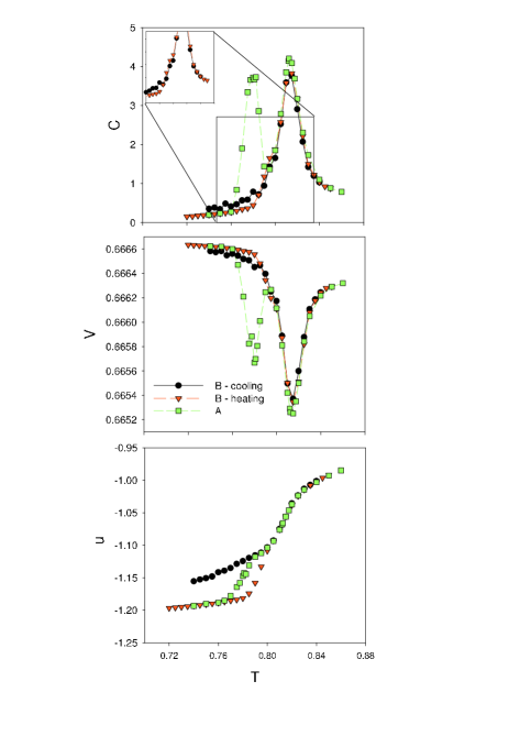
Figure 1: (Color on-line) Specific heat $C$, fourth order cumulant $V$ and internal energy per spin $u$ as a function of temperature for $J/g=4$ ($\delta=2$) and $L=48$, obtained from different MC simulation protocols (see text for details).

Moreover, we showed that the finite size scaling of the different thermodynamical quantities around the nematic-tetragonal phase transition are consistent with a first order transition, while those observed around the stripe-nematic transition present unusual features, some of them resembling a Kosterlitz-Thouless one (like a saturation in the specific heat maximum and a continuous change in the internal energy) while others are also characteristic of a first order phase transition. In particular, one of those characteristics is the existence of diverging free energy barriers between the nematic and the stripe phases, which generate a strong meta–stabilities when the system is cooled or heated through the transition temperature. To correctly characterize the finite size scaling at this phase transition thermodynamical quantities must be averaged for every temperature over a large single MC run, thus allowing the system to sample properly the different phases. Otherwise, as explained by Challa et alChalla et al. (1986), the first-order character of the transition introduces pronounced meta–stabilities with the system spending most of the time in one of the two phases (see Ref.Challa et al. (1986) for details). Hence, for every temperature we first let the system run over a transient period of $M_{1}$ Monte Carlo Steps (MCS) and then we averaged the different quantities over a single MC run of $M_{2}$ MCS, with $M_{1}$ ranging between $10^{6}$ and $2\times 10^{7}$, and $M_{2}$ ranging between $2\times 10^{7}$ and $2\times 10^{8}$; we shall call this procedure protocol A. We believe that the absence of the nematic-stripe phase transition (and therefore the evidence of the nematic phase) in Rastelli et al paper is due to the particular MC protocol they used, which introduced a strong bias in their results. They took averages over eight independent MC runs of $10^{5}$ MCS for each temperature, taking the initial configuration for every temperature as the final configuration of the previous one, disregarding $10^{4}$ MCS for thermalizationRastelli et al. (2006); we shall call this procedure protocol B. This protocol is similar to a finite rate heating (cooling) procedure from low (high) temperature and the system can get trapped in the meta–stable striped (nematic) state, thus hiding the low temperature phase transition, whose associated free energy barriers are very high for system sizes used in that work. Indeed we checked this assumption by computing the moments of the energy, namely the internal energy per spin $u$, the specific heat $C$ and the fourth order cumulant $V$ as a function of the temperature (see definitions in Ref.Cannas et al. (2006)) using Rastelli et al MC protocol for $\delta=2$ and $L=48$, both heating from the low temperature stable phase and cooling from the high temperature one. The results were averaged over $8$ (as in Rastelli et al paper) and $50$ independent runs; no qualitative differences were observed. The obtained results for $50$ independent runs are compared in Fig.1 with the results obtained in Ref.Cannas et al. (2006) for the same parameters values.

We see that the low temperature maximum of $C$ and the minimum of $V$ are almost undetectable by Rastelli et al MC protocol, the only noticeable effect being some enlarged fluctuations in the cooling procedure and a very small shoulder for the heating result at the left of the high temperature specific heat maximum (the inset of Fig.1 remarks this effect) or cumulant minimum, but clearly separated from the actual low temperature transition. Moreover, the behavior of $u$ shows clearly that the system gets trapped in a metastable super-cooled (super-heated) state, as in a finite rate cooling (heating) process (compare with Fig.19 in Ref.Cannas et al. (2006)). Indeed we observed that for some individual runs in the heating procedure the specific heat presents a small secondary maximum of the specific heat at low temperatures, but those maxima are a result of a spinodal instability of the super-heated state and therefore are strongly shifted to the right of the actual maximum. Moreover, those spinodal maxima appear located at different random temperatures and they are smeared out when averaged, giving rise to the observed shoulder.

Even when the analysis in Ref.Cannas et al. (2006) was carried out for the particular value $\delta=2$, theoretical resultsKashuba and Pokrovsky (1993); Abanov et al. (1995) lead us to expect the presence of the nematic phase to be found for a wide range of values of $\delta$, although possibly for even narrower ranges of temperatures than for $\delta=2$. In that case, the above described spurious effects should become worse. Indeed, the nematic phase and the associated behavior in the specific heat and cumulant has been foundPiC using protocol A for other values of $\delta$, including $\delta=2.25$ ($J/g=4.5$), which corresponds to the $h=3$ ground state region, as the $J/g=5$ case analyzed by Rastelli et al (and close to it).

Another related point concerns the scaling of the principal maximum of $C$ for $J/g=5$ in Rastelli et al work. They found that the maximum scales as $~{}L^{1.2}$ instead of the $L^{2}$ scaling expected in a first order transition. A careful analysis of the orientational order parameter histogram for $\delta=2$ shows the presence of multiple peaks around this transition (See Fig.7 in Ref.Cannas et al. (2006)) indicating the presence of a complex multiple phase structure in a very narrow range of temperatures; such structure is only detectable for large system sizes and can introduce a strong bias in the scaling properties for small sizes. The anomalous scaling observed by Rastelli et all is probably due to this finite size effect.

The above considerations also apply to the case $J/g=6$. In this case the results of Rastelli et al (see Fig.12 in Ref.Rastelli et al. (2006)) show rather clearly the presence of a secondary low temperature peak in the specific heat, whose height is independent of the system size, very similar to that observed for $J/g=4$ (see Fig.9 in Ref.Cannas et al. (2006)). There is also some indication of a vanishing secondary minimum in $V$, similar to that observed for $J/g=4$. Although those anomalies are very small, they are probably affected also by the simulation protocol and by finite size effects, which in this system become stronger as $J/g$ increases. Based on the scaling of the specific heat maximum and on the apparently vanishing minimum of the energy cumulant the authors conclude that the transition is continuous for $J/g\geq 6$. However, such results can also be consistent with a weak first order transition that continuously fades out as $J/g$ increases. If that would be the case, detecting the order of the transition becomes more delicate due to the above described finite size effects. Indeed, a Hartree approximation applied to the continuous version of Hamiltonian (1) predicts a first order transition for a wide range of values of Cannas et al. (2004) $J/g$. Rastelli et al criticize this result claiming that such approximation wrongly predicts a first order transition also for $g=0$, where it is known that it is second order. As is well known since the work by Brazovskii S. A. Brazovskii (1975), that calculation breaks down for $g=0$. Nevertheless, for a wide range of values of $J/g>1$ the approximation gives excellent qualitative results. It is at least very suggestive that our numerical results seem to be in agreement with the predictions of this theory. To be more specific, at the transition a modulated solution of the form $\phi(\vec{r})=m\cos{(\vec{k_{0}}\cdot\vec{r})}$ becomes stable and the amplitude of the equilibrium solution $m(T)$ jumps discontinously to a non zero value. Following Brazovskii S. A. Brazovskii (1975) it is possible to show that the amplitude at the transition is given by

$$m_{c}=m(T_{c})\propto\sqrt{r_{m}(T_{c})/u},$$ (2)

where $u$ is the coupling constant of the Landau energy and $r_{m}$ is the renormalized mass of the modulated solution Cannas et al. (2004). At the transition point $r_{m}\propto(u\,k_{0}^{2})^{2/3}$ and

$$m_{c}\propto\frac{k_{0}^{2/3}}{u^{1/6}}$$ (3)

In our model $k_{0}\propto g/J$ and consequently the amplitude at the transition decreases continuously as $g/J$ gets smaller within the range of validity of the approximation. This shows that the transition becomes weaker as $g/J$ diminishes. This is completely consistent with the difficulty in the numerical simulations to detect the first order nature of the transition for small values of $g/J$.

Finally, for $J/g=1.7$, Rastelli et al found evidence of a continuous phase transition with unusual critical exponents, from which they conclude that the $h=1$ spin configurations ($h$ being the width of the ground state stripes) undergo a continuous phase transition with a different universality class from the case $J=0$. In Ref.Cannas et al. (2006) we presented evidence that the system undergo a unique weak first order transition for $J/g=2$ ($\delta=1$); this value of the ratio also corresponds to the $h=1$ region of the phase diagram (see phase diagram in Gleiser et al. (2003)). These results are consistent with the presence of a second order transition line for small values of $J/g$ that joins with continuous slope a first order transition line for larger values of $J/g$ at a tricritical point in that region of the phase diagram (see phase diagram in Gleiser et al. (2003)). Hence, the unusual critical exponents observed by Rastelli et al are most probably due to a crossover effect related to the presence of that tricritical point in the neighborhood of $J/g=1.7$ and not to a new universality class transition line.

This work was partially supported by grants from CONICET (Argentina), Agencia Córdoba Ciencia (Argentina), SeCyT, Universidad Nacional de Córdoba (Argentina), CNPq (Brazil) and ICTP grant NET-61 (Italy).

References

- Rastelli et al. (2006) E. Rastelli, S. Regina, and A. Tassi, Phys. Rev. B 73, 144418 (2006).
- De’Bell et al. (2000) K. De’Bell, A. B. MacIsaac, and J. P. Whitehead, Rev. Mod. Phys. 72, 225 (2000).
- Cannas et al. (2006) S. A. Cannas, M. F. Michelon, D. A. Stariolo, and F. A. Tamarit, Phys. Rev. B 73, 184425 (2006).
- Kashuba and Pokrovsky (1993) A. B. Kashuba and V. L. Pokrovsky, Phys. Rev. B 48, 10335 (1993).
- Abanov et al. (1995) A. Abanov, V. Kalatsky, V. L. Pokrovsky, and W. M. Saslow, Phys. Rev. B 51, 1023 (1995).
- Challa et al. (1986) M. S. S. Challa, D. P. Landau, and K. Binder, Phys. Rev. B 34, 1841 (1986).
- (7) S. A. Pighin and S. A. Cannas, to be published.
- Cannas et al. (2004) S. A. Cannas, D. A. Stariolo, and F. A. Tamarit, Phys. Rev. B 69, 092409 (2004).
- S. A. Brazovskii (1975) S. A. Brazovskii, Sov. Phys. JETP 41, 85 (1975).
- Gleiser et al. (2003) P. M. Gleiser, F. A. Tamarit, S. A. Cannas, and M. A. Montemurro, Phys. Rev. B 68, 134401 (2003).