SU(4) composite fermions in graphene: New fractional quantum Hall states

Abstract

Theoretical studies of the fractional quantum Hall effect (FQHE) in graphene have so far focused on the plausibility and stability of the previously known FQHE states for the interaction matrix elements appropriate for graphene. We consider FQHE for SU(4) symmetry, as appropriate for the situation when all four spin and valley Landau bands are degenerate, and predict new FQHE states that have no analog in GaAs. These result from an essential interplay between the two-fold spin and valley degeneracies at fractions of the form $\nu=n/(2pn\pm 1)$, for $n\geq 3$. Conditions are outlined for the observation of these states and quantum phase transitions between them; the structure of these states and their excitations is also described.

I Introduction

Soon after the first experimental realization of graphene, a single-layer hexagonal form of carbon, the integral quantum Hall effect (IQHE)Klitzing80 was observed by Novoselov et al. and Zhang et al.Novoselov at filling factors $\nu_{n}=4n-2$. The $\Delta\nu=4$ period is understood straightforwardly as a consequence of the four-fold (near) degeneracy of Landau levels (LLs) in graphene; the Zeeman energy is small in comparison to the interaction energy scale, and the pseudospin degree of freedom, which represents the two inequivalent Dirac-cones at the corners of the Brillouin zone, does not couple to external fields if the two sublattices are equivalent. The offset $-2$ is a consequence of a Dirac-like effective Hamiltonian, which produces a linear dispersion for low energy electronic states Semenoff . Recently, Zhang et al.Zhang have observed quantum Hall plateaus at $\nu=\pm 4,\pm 1,0$. Although external effects can surely lift the four-fold degeneracy of the low-lying LLs, Yang, Das Sarma and MacDonaldYang have shown that the exchange interaction can break the SU(4) symmetry spontaneously, and the charged excitations are skyrmions Skyrmion in the $|n|\leq 3$ Landau levels at $\tilde{\nu}=1$ (or, by particle-hole symmetry, at $\tilde{\nu}=3$) where $\tilde{\nu}=\nu-\nu_{n}$ is the filling factor within the Landau level in question. This has been confirmed FQHEgraphene by exact diagonalization for $n\leq 2$ with $N\leq 9$ particles.

Although the fractional quantum Hall effectTsui82 (FQHE) has not yet been observed in graphene, it has been explored theoretically FQHEgraphene ; Apalkov assuming an SU(2) symmetry, as appropriate, for example, when the Zeeman energy is sufficiently high that only the two-fold pseudospin degeneracy remains. In this situation, the graphene FQHE problem formally maps into the well studied problem of FQHE in GaAs in the zero Zeeman energy limitWu93 ; Park1 , with the pseudospin of the former playing the role of the spin of the latter. In the $n=0$ graphene LL, the interaction pseudopotentialsHaldane are identical to those in GaAs, so the mapping is perfect, and the earlier composite-fermion results of Refs. Wu93, ; Park1, carry over to graphene with minimal change (spin replaced by pseudospin). In particular, it follows that FQHE occurs at fractional fillings given by $n/(2pn\pm 1)$, with pseudospin singlet states at even $n$ and pseudospin polarized states at odd $n$ (fully pseudospin polarized for $n=1$), terminating into a pseudospin singlet composite fermion Fermi sea in the limit of $n\rightarrow\infty$ ($\tilde{\nu}=1/2p$). The effective interaction in the $n\neq 0$ LLs in graphene interpolates between those of the $|n|$th and $(|n|-1)$st LLs for the quadratic dispersion; the composite fermion formationJain89 , and therefore the FQHE, are found to be almost as strong in the $|n|=1$ LL in graphene as in the lowest LL of GaAs FQHEgraphene .

It is natural to wonder if FQHE with new structure appears in graphene. For this purpose, we explore in this work FQHE including the full SU(4) symmetry. By a combination of exact diagonalization and the CF theory, we find new FQHE states which result from an essential interplay between the spin and the pseudospin degrees of freedom; such states occur at $\tilde{\nu}=n/(2n+1)$ for $n\geq 3$. For other states, the energy spectrum of the SU(4) problem matches with that of the SU(2) problem, although the multiplicities are vastly different. We show by exact diagonalization that the SU(4) symmetry is spontaneously broken at $\tilde{\nu}=\frac{1}{3}$ just as at $\tilde{\nu}=1$, i.e., the orbital part of the ground state is antisymmetric and the excitations are skyrmionic. At $\tilde{\nu}=\frac{1}{3},\frac{2}{3}$ and $\frac{2}{5}$, the orbital part of ground state is the same as in the SU(2) symmetric system, but the state is now a highly degenerate SU(4) multiplet.

The outline of the paper is as follows. We review the methods in Sec. II. In Sec. III we generalize the composite fermion theory to SU(4) electrons, using Fock’s condition and constructing all possible wave functions of incompressible, filled $\Lambda$ level states of composite fermions. We also indicate which states have analogs in GaAs and which do not. Section IV is concerned with exact diagonalization results for small systems, which are compared to the predictions of the CF theory. Skyrmion-like excitations are also discussed. In Sec. V we obtain thermodynamic energies using the CF theory to determine the thermodynamic ground states. Section VI discusses zero-temperature phase transitions and lists the CF predictions for the parameters where the new FQHE states should be observable. The paper is concluded in Section VII.

II Model

The electronic structure of graphene is well described by a tight binding modelSemenoff , which gives a vaulted band structure with the valence and conductance bands touching in the symmetry protected Dirac (or Fermi) points at the six corners of the hexagonal Brillouin zone. The low energy states, in particular, occupy double conesCones with apices at the corners. Only two of these six double cones are inequivalent, giving rise to a pseudospin degree of freedom. Denoting spin by $\vec{S}$ and pseudospin by $\vec{P}$, the low energy states are described in the continuum approximation by an effective HamiltonianSemenoff

$$H=v_{F}\begin{pmatrix}\vec{\sigma}\cdot\vec{\Pi}&0\\ 0&(\vec{\sigma}\cdot\vec{\Pi})^{\textrm{T}}\\ \end{pmatrix}+\Delta P_{z}+g\mu_{B}\vec{B}\cdot\vec{S},$$ (1)

that acts on a 4-spinor Hilbert space. Here $v_{F}\approx 10^{6}$ m/s is the Fermi velocity, $\vec{\Pi}=\vec{p}+\frac{e}{c}\vec{A}$, $\Delta$ is the on-site energy difference between the two sublattices, $P_{i}=1\otimes\frac{1}{2}\sigma_{i}$ is the pseudospin operator, and $\vec{S}$ is the spin. Letting $z=x-iy$, measuring distance in units of the magnetic length $\ell_{B}=\sqrt{\hbar c/eB}$, and using the symmetric gauge $\vec{A}=(-By/2,Bx/2)$, this Hamiltonian is diagonalized by the normalized eigenvectors

$$\Psi^{(0,m)}_{p=1/2,s} = \begin{pmatrix}0\\ \eta_{0,m}\\ 0\\ 0\end{pmatrix}\otimes\alpha_{s},$$ (2)

$$\Psi^{(0,m)}_{p=-1/2,s} = \begin{pmatrix}0\\ 0\\ \eta_{0,m}\\ 0\end{pmatrix}\otimes\alpha_{s},$$ (3)

$$\Psi^{(n\neq 0,m)}_{p=1/2,s} = \frac{1}{\sqrt{2}}\begin{pmatrix}-{\rm sgn}(n)i\eta_{|n|-1,m}\\ \eta_{|n|,m}\\ 0\\ 0\end{pmatrix}\otimes\alpha_{s},$$ (4)

$$\Psi^{(n\neq 0,m)}_{p=-1/2,s} = \frac{1}{\sqrt{2}}\begin{pmatrix}0\\ 0\\ \eta_{|n|,m}\\ -{\rm sgn}(n)i\eta_{|n|-1,m}\end{pmatrix}\otimes\alpha_{s},$$ (5)

where $\alpha_{1/2}=\begin{pmatrix}1\\ 0\end{pmatrix}$, $\alpha_{-1/2}=\begin{pmatrix}0\\ 1\end{pmatrix}$, and $\eta_{n,m}$ is the eigenstate of the Hamiltonian with quadratic dispersion in LL $n$ with angular momentum ($L_{z}$) equal to $m$:

$$\eta_{n,m}(z)=\frac{(-1)^{n}\sqrt{n!}}{\sqrt{2^{m+1}\pi(m+n)!}}z^{m}L_{n}^{m}\left(\frac{|z|^{2}}{2}\right)e^{-|z|^{2}/4}.$$ (6)

The corresponding energies are

$$E_{nps}={\rm sgn}(n)\sqrt{\frac{2\hbar v_{F}^{2}eB|n|}{c}}+\Delta p+g\mu_{B}Bs.$$ (7)

In the limit $g\to 0,\Delta\to 0$, the four vectors

$$\Psi^{(n,m)}_{1/2,1/2},\quad\Psi^{(n,m)}_{1/2,-1/2},\quad\Psi^{(n,m)}_{-1/2,1/2},\quad\Psi^{(n,m)}_{-1/2,-1/2}$$ (8)

are degenerate, giving rise to an SU(4) internal symmetry.

The SU(4) approximation is valid if $E_{Z}=g\mu_{B}B$ and $\Delta$ are small in comparison to the scale of the interactions, $e^{2}/(\epsilon l_{B})$. While $\Delta$ is not easy to estimate, it is generally believed to be much smaller than $E_{Z}$. One can check that

$$E_{Z}\left/\left(\frac{e^{2}}{\epsilon l_{B}}\right)\right.=0.001\epsilon g\sqrt{B[\text{T}]},$$

where $B[\text{T}]$ is the magnetic field in Tesla. Obviously, both $\epsilon$ and $g$ depend strongly on the interaction with environment in which the graphene sheet is placed. As two extremes, one can take $\epsilon_{\text{min}}=(\epsilon_{\text{air}}+\epsilon_{\text{SiO}_{2}})/2=2.75$ and $\epsilon_{\text{max}}=15$ (the graphite value). On the other hand, Zhang et al. Zhang find $1.7\leq g\leq 2.0$. With these extreme values, assuming an extremely high field $B=45$ T, we get

$$\left(E_{Z}\left/\left(\frac{e^{2}}{\epsilon l_{B}}\right)\right.\right)_{\text{min}} = 0.032,$$

$$\left(E_{Z}\left/\left(\frac{e^{2}}{\epsilon l_{B}}\right)\right.\right)_{\text{max}} = 0.208.$$

Thus the SU(4) symmetric approximation is typically valid unless $\epsilon$ happens to be close to the high end of the estimation.

The interaction between eigenstates is conveniently described in terms of pseudopotentialsHaldane , where the pseudopotential $V_{m}$ gives the energy of two electrons in relative angular momentum $m$. As a consequence of Eqs. (2) and (4), the problem of interacting electrons in the $n$th LL of graphene can be mapped into a problem of interacting electrons in $\eta_{0,m}$ states with effective pseudopotentialsApalkov ; FQHEgraphene

$$V_{m}^{(n)\textrm{gr.}}=\int\frac{d^{2}k}{(2\pi)^{2}}\frac{2\pi}{k}F_{n}(k)e^{-k^{2}}L_{m}(k^{2}),$$ (9)

where the form factor $F_{n}$ is

$$F_{0}(k)=1,\quad F_{n}(k)=\frac{1}{4}\left(L_{n}\left(\frac{k^{2}}{2}\right)+L_{n-1}\left(\frac{k^{2}}{2}\right)\right)^{2}.$$ (10)

The problem of interacting electrons is conveniently formulated in the spherical geometry, in which electrons move on the surface of a sphere and a radial magnetic field is produced by a magnetic monopole of strength $Q$ at the center.Haldane ; Fano Here $2Q\phi_{0}$ is the magnetic flux through the surface of the sphere; $\phi_{0}=hc/e$, and $2Q$ is an integer according to Dirac’s quantization condition.Dirac31 For quadratic dispersion the single particle states are monopole harmonicsYang1976 $Y_{Qlm}$, where $l=Q+n$ is the angular momentum with $n=0,1,\ldots$ being the LL index, $m=-l,-l+1,\ldots,l$ is the $z$-component of angular momentum. The Coulomb interaction is evaluated with the chord distance. The analogous solution for carriers with linear dispersion, described by the massless Dirac’s equation, is not known for the spherical geometry. We proceed to work in the basis of the monopole harmonics $Y_{QQm}$ of the lowest LL, while using the effective pseudopotentials given in Eq. (9). Because we have $F_{0}(k)=1$, in the $n=0$ Landau level the pseudopotentials derived by Fano et al.Fano can be used. In other Landau levels, however, we will use the effective pseudopotentials of the planar geometry (Eq. (9)) on the sphere. Such an identification is obviously exact in the thermodynamic limit, but is usually reasonable also for finite systems.

We neglect the finite thinkness of the two dimensional electron system, which is a much better approximation in graphene than in GaAs heterostructures. The neglect of Landau level mixing, also made below, is a more tricky assumption because both the LL separation (c.f. Eq. (7)) and the interaction energy scale as $\sqrt{B}$, and are of the same order. However, their relative strengths can be controlled by variation of other parameters (Fermi velocity, dielectric constant, etc.), and we will assume in the following that the LL separation is large enough to suppress LL mixing.

III Composite fermion theory for SU(4) electrons

We will compare the exact diagonalization results to the composite fermion theory Jain89 ; JainKamilla , and also use this theory to explore the thermodynamic limit. (Exact diagonalization can be performed only for very small systems for SU(4) symmetry.) The composite fermion (CF) theory maps the strongly interacting system of electrons in a partially filled Landau level to a system of weakly interacting particles called composite fermions, which are bound states of an electron and an even number of quantized vortices. The mapping consists of attaching $2p$ quantized vortices of the many-body wave function to each electron. The quantized vortices produce Berry phases that partly cancel the external magnetic field, and consequently composite fermions feel a reduced magnetic field $B^{\ast}=B-2p\rho\phi_{0}$. Composite fermions in magnetic field $B^{\ast}$ fill quantized kinetic energy levels analogous to Landau levels, called $\Lambda$ levels. If $m$ $\Lambda$ levels are filled, which corresponds to a filling factor $\nu=\frac{m}{2pm\pm 1}$, an incompressible quantum liquid state results. The FQHE is thus explained as the IQHE of composite fermions.

According to the CF theory, the wave functions for correlated electrons in the lowest Landau level at monopole strength $Q$ are given by

$$\Psi=P_{\rm LLL}\Phi_{1}^{2p}\Phi,$$ (11)

$$\Phi_{1}=\prod_{j<k}(u_{j}v_{k}-v_{j}u_{k}),$$ (12)

where $\Phi$ is a wave function for $N$ non-interacting electrons at monopole strength $q=Q-p(N-1)$, operator $P_{\rm LLL}$ projects a state into the $n=0$ LL, and $u=\cos(\theta/2)e^{-i\phi/2}$ and $v=\sin(\theta/2)e^{i\phi/2}$. The procedure taking us from $\Phi$ to $\Psi$ is called “composite-fermionization,” which also converts electronic Landau levels into $\Lambda$ levels of composite fermions. Incompressible ground states are constructed by completely filling the lowest few $\Lambda$ levels in one or more spin bands. The explicit relation between the monopole strength $Q$, the filling factor $\tilde{\nu}$ and the particle number $N$ is given below in Eq. (16).

III.1 Fock’s condition

The above CF construction is valid for the orbital part of the wave function independent of whether the Landau levels are singly, doubly, or quadruply degenerate, i.e., whether the low-energy electronic states have no internal (nonorbital) symmetry, have SU(2) symmetry, or have SU(4) symmetry, respectively. However, while any antisymmetric wave function is valid for a singly degenerate Landau level, only those wave functions are legitimate for SU(2) which are eigenstates of $S^{2}$ and $S_{z}$. For SU($n$) electrons, the wave functions are eigenfunctions of all the Casimir operators and the generators of the Abelian subalgebra of the Lie algebra of SU($n$). Among such functions the so-called maximal weight statesSymm satisfy Fock’s cyclic conditionHamermesh . The idea will be to construct valid IQHE wave functions $\Phi$, and then show that their “composite fermionization” produces FQHE wave functions with valid symmetry.

Fock’s cyclic condition tells us which orbital wave functions are legitimate for the highest weight state in the multiplet $[m_{1},\dots,m_{n-1}]$ of SU($n$). We are using the Young tableau notation for the SU($n$) multiplets: $m_{1}\geq m_{2}\geq\dots m_{n-1}\geq 0$ are integers, $m_{i}$ being the length of the $i$-th row of the Young tableau of the representation. (The last $m_{i}$’s are omitted if zero.) Recall that Young tableaux are generated from the direct products of the fundamental representation (a single box) with symmetrization in the rows and antisymmetrization in the columns.

Let $\{\alpha^{t}\}$ be a basis of the ($n$-dimensional) fundamental representation of SU($n$), and let $M_{t}$ be the number of particles assumed to be in the $\alpha^{t}$ internal state. Let

$$\Phi^{\prime}(\{\vec{r}_{j}\})={\cal A}\left(\Phi(\{\vec{r}_{j}\})\prod_{t=1}^{n}\prod_{i=\min_{t}}^{\max_{t}}\alpha^{t}_{i}\right),$$ (13)

where $\min_{1}=1,\max_{1}=M_{1},\min_{2}=M_{1}+1,\max_{2}=M_{1}+M_{2},\dots$, and $\cal A$ is the antisymmetrizer. Assume $\Phi(\{\vec{r}_{j}\})$ is antisymmetric in each subset $\{\min_{t},\dots,\max_{t}\}$ of its variables. $\Phi^{\prime}(\{\vec{r}_{j}\})$ is a highest weight state (w.r.t. a choice of positive roots) if and only if it is annihilated by any attempt to antisymmetrize an electron $l$ of type $u$ ($\min_{u}\leq l\leq\max_{u}$) with respect to the electrons of type $t<u$, i.e.

$$\left(e-\sum_{k=\min_{t}}^{\max_{t}}(k,l)\right)\Phi(\{\vec{r}_{j}\})=0,$$ (14)

where $e$ is the identity and $(k,l)$ permutes indices $k$ and $l$.

Consequently, any orbital wavefunction

$$\Phi=\Phi_{1}\Phi_{2}\cdots\Phi_{n},$$ (15)

where $\Phi_{s}$’s are Slater determinants such that any state $(n,m)$ in $\Phi_{s}$ is also filled in $\Phi_{s-1}$ (conversely, if $(n,m)$ is empty in $\Phi_{s}$, then it is also empty in $\Phi_{s+1}$), is a legitimate highest weight wave function for SU($n$). This class includes IQHE states ($\Psi_{s}$ has the lowest $l_{s}$ Landau level completely filled; $l_{s}$’s are in decreasing order), Fermi sea states, and single particle, single hole, and particle-hole pair states above the IQHE and Fermi sea states, provided that no hole is created in spin state $s$ in a LL that is filled in $\Phi_{s+1}$, and, conversely, no particle is created in spin state $s$ in a LL that is unfilled in $\Phi_{s-1}$.

If state $\Phi$ satisfies Fock’s condition (14), so does $\Psi$ given by Eq. (11), and is therefore a legitimate state. Thus composite fermion states with parallel or antiparallel flux attachment can be constructed from electronic Hartree-Fock states as usual. The CF theory for SU(2) systems thus generalizes trivially to SU($n$) systems.

III.2 New FQHE states

These observations enable us to construct variational wave functions for $\tilde{\nu}=\frac{m}{2pm\pm 1}$. For $m=1$, a single filled $\Lambda$ level (in one of the $\alpha^{t}$ spin bands) is the only candidate for an incompressible ground state; the SU(4) multiplet is $[N]$. For $m=2$, the two $\Lambda$ levels are filled with particles of identical or different spin state; the multiplet is $[N]$ or $[N/2,N/2]$, respectively. As the restriction on the orbital part of the CF wave functions is identical to the SU(2) case, we expect the latter is prefered in the absence of a symmetry-breaking field.

Figure 1: The construction of composite fermion ground states for fractions where four $\Lambda$-levels can be filled ($\tilde{\nu}=\frac{4}{9}$, $\frac{4}{7}$, etc). While the top three states are possible in SU(2) systems, the lowest two require an SU(4) symmetric internal degree of freedom. The filled and empty arrows indicate the $z$-component of the spin $S_{z}$ and the pseudospin $P_{z}$, respectively. This construction remains valid when $S^{\prime}_{z}$ and $P^{\prime}_{z}$ replace $S_{z}$ and $P_{z}$ (c.f. Eq. (19)). The top three states also occur in GaAs; the bottom three are new.

For $m\geq 3$, however, the SU(4) internal degree of freedom allows new ground state candidates. Let $(l_{1},l_{2},l_{3},l_{4})$ denote a trial wave function that fills $l_{1},\dots,l_{4}$ $\Lambda$ levels of the different single particle spin states. As an example, Fig. 1 depicts all such states for $m=4$. (For the monopole strength in finite spherical models, see Eq. (16) below.) Which of these states will be the ground state will be determined only by detailed microscopic calculations (to be described below). A mean field approximation, which has been found to be successful for SU(2) electrons Wu93 ; Park1 , predicts that the state with the lowest “CF kinetic energy” is the ground state. This approximation, however, neglects the residual interaction between composite fermions, which favors the maximally polarized state due to exchange contribution.

IV Exact diagonalization results

IV.1 Ground states

Table 1 shows the angular momentum and the SU(4) multiplet of the ground state in the $|n|=0,1$ Landau levels at flux values given by

$$2Q=2p(N-1)\pm\left(\frac{N-\sum_{i}l_{i}^{2}}{m}\right),$$ (16)

where the $(l_{1},l_{2},l_{3},l_{4})$ state is a candidate for the ground state at $\tilde{\nu}=\frac{m}{2pm\pm 1}$ with $m=\sum_{i}l_{i}$. The following observations are consistent with the CF theory:

1. All ground states at the $N$ and $Q$ values satisfying Eq. (16) have rotational symmetry ($L=0$), consistent with the CF theory expectation of incompressibility for these parameters $N$ and $2Q$. These systems therefore are finite size representations of incompressible states at $\tilde{\nu}=\frac{m}{2pm\pm 1}$.

2. The filling $\tilde{\nu}=\frac{1}{3}$ corresponds to $m=1$, a single filled $\Lambda$ level (in one of the $\alpha^{t}$ spin bands) is the only candidate for an incompressible ground state; the SU(4) multiplet is $[N]$, which is consistent with Table 1. The energy is identical to the SU(2) case, but the multiplicity of the ground state is different ($\approx N^{3}/6$). Analogous to $\tilde{\nu}=1$, the ground state is a completely symmetric $[N]$ multiplet, which has associated with it a fully antisymmetric orbital wave function, in accordance with the Pauli’s principle. This is the SU(4) equivalent of the well-known ferromagnetic behavior in systems with quadratic dispersion relation (GaAs heterostructures and quantum wells) in the vanishing Zeeman energy limit. Unlike in the SU(2) symmetric case, however, the spins are not necessarily aligned in the same direction; in the $[N]$ multiplet spin and pseudospin are equal, but they can take all of the possible valuesQuesne ; Hecht : $S=P=0,1,\dots,\frac{N}{2}$ if $N$ is even, and $S=P=\frac{1}{2},\frac{3}{2},\dots,\frac{N}{2}$ if $N$ is odd. (The total multiplicity comes from these choices combined with the choice of $P_{z}$ and $S_{z}$.) Any weak perturbation that polarizes the spin should also polarize the pseudospin.

3. For $m=2$, two $\Lambda$ levels are filled with particles of identical or different spin state; the multiplet is $[N]$ or $[N/2,N/2]$, respectively. As the orbital part of the CF wave functions is identical to the SU(2) case, it is no surprise that the latter is prefered in the absence of a symmetry-breaking field (c.f. the $\nu=\frac{2}{3},\frac{2}{5}$ data in Table 1). (The multiplicity of $[\frac{N}{2},\frac{N}{2}]$ is $\approx N^{4}/96$.) The ground state energy is the same as in the SU(2) symmetric case. In Sec. III it was shown that the maximal weight state is a product of two Slater determinants just as for an SU(2) singlet. Because the SU(2) systems already find the lowest energy state in this class, the orbital part of the wave function remains the same. However, the ground state is neither a spin nor a pseudospin singlet; all spin $S$ and pseudospin $P$ combinations occur with $(S+P)=0,2,\dots,\frac{N}{2}$ for $N$ even, and $(S+P)=1,3,\dots,\frac{N}{2}$ for $N$ odd.

4. At $\tilde{\nu}=\frac{3}{7}$ and $\tilde{\nu}=\frac{4}{9}$, the $n=0$ LL ground state multiplets are consistent with three and four copies of completely filled lowest $\Lambda$ levels, respectively, consistent with the expectation from the mean-field model. (Notice that $[N/3,N/3,N/3]$ and $[N/4,N/4,N/4,N/4]$ are conjugate representations to $[N/3]$ and $[0]$, respectively, which cannot be distinguished by their $(S,P)$ quantum numbers.) The mean-field expectation is not borne out in the $|n|=1$ LL. In Sec. III, however, we have seen that new composite fermion ground states become possible at these fractions; the small system calculations we can perform at $\tilde{\nu}=\frac{3}{7}$ and $\tilde{\nu}=\frac{4}{9}$ are unable to determine the true nature of the ground states at these fractions.

$\tilde{\nu}$	$N$	$2Q$	$D$	$L^{(0)}$	$SU(4)$ m.	$L^{(1)}$	$SU(4)$ m.
$\frac{1}{3}$	4	9	960	0	[4]	0	[4]
	5	12	12934	0	[5]	0	[5]
	6	15	282824	0	[6]	0	[6]
$\frac{2}{3}$	4	5	204	0	[2,2]	0	[2,2]
	6	8	14464	0	[3,3]	0	[3,3]
$\frac{2}{5}$	4	7	488	0	[2,2]	0	[2,2]
	6	12	97316	0	[3,3]	0	[3,3]
$\frac{3}{7}$	3	4	27	0	[1]	0	[1]
	6	11	64392	0	[2]	0	[4]
$\frac{4}{9}$	4	6	325	0	[0]	0	[4]

Table 1: Orbital angular momentum $L^{(n)}$ and $SU(4)$ multiplet of the ground states of finite systems on a sphere at the most prominent fractions in the $n=0$ and $|n|=1$ Landau levels of graphene. The quantity $\tilde{\nu}$ is the filling factor within the Landau level; $Q$ is the monopole strength; $N$ is the number of electrons; and $D$ is the dimension of the Hilbert space in the $L_{z}=S_{z}=P_{z}=0$ sector.

IV.2 Charged excitations: SU(4) CF skyrmions

For SU(2) symmetry and vanishing Zeeman energy, the charged excitations at $\nu=1/3$, which map into filling factor one of composite fermions, are skyrmions of composite fermions CFSkyrmion . These are analogous to skyrmions of electrons Skyrmion at $\nu=1$. The skyrmions at these fillings are obtained as the ground states with the monopole strength $Q$ changed by $\pm 1$ relative to the $Q$ of the sequence representing the state at $\tilde{\nu}$. As Tables 2 and 3 testify, near $\tilde{\nu}=\frac{1}{3}$, these states belong to an $\left[\frac{N}{2},\frac{N}{2}\right]$ or an $\left[\frac{N+1}{2},\frac{N-1}{2}\right]$ multiplet, depending on whether $N$ is even or odd. (The degeneracies of these multiplets are $\approx N^{4}/96$ and $\approx N^{4}/48$, respectively.) We identify these states with SU(4) composite fermion skyrmions. The energies of these states are identical to the familiar SU(2) skyrmions, as these spinors enforce (cf. Sec. III) exactly the same partition of the wave function into antisymmetric factors as the SU(2) singlet ($N$ even) or spin-$\frac{1}{2}$ ($N$ odd). Consequently, the gaps at $\tilde{\nu}=\frac{1}{2p+1}$ are identical to those calculated with SU(2) symmetryFQHEgraphene ; CFSkyrmion : $\Delta_{1/3}^{(0)}=0.043(5)e^{2}/\epsilon l_{B}$ and $\Delta_{1/3}^{(1)}=0.017(3)e^{2}/\epsilon l_{B}$.

$\tilde{\nu}$	$N$	$2Q$	$D$	$L^{(0)}$	$SU(4)$ m.	$L^{(1)}$	$SU(4)$ m.
1	4	2	25	0	[2,2]	0	[0,0]
	5	3	92	$\frac{1}{2}$	[3,2]	$\frac{1}{2}$	[3,2]
	6	4	644	0	[3,3]	0	[3,3]
	7	5	3236	$\frac{1}{2}$	[4,3]	$\frac{1}{2}$	[4,3]
	8	6	24483	0	[4,4]	0	[4,4]
	9	7	142587	$\frac{1}{2}$	[5,4]	$\frac{1}{2}$	[5,4]
$\frac{1}{3}$	4	8	697	0	[2,2]	0	[2,2]
	5	11	9296	$\frac{1}{2}$	[3,2]	$\frac{1}{2}$	[3,2]
	6	14	203132	0	[3,3]	0	[3,3]

Table 2: Orbital angular momentum $L^{(n)}$ and $SU(4)$ multiplet of the ground states of finite systems on the sphere on the quasiparticle side of $\nu=1$ and $\frac{1}{3}$ in the $n=0$ and $|n|=1$ Landau levels of graphene. $D$ is the dimension of the Hilbert space in the $L_{z}=S_{z}=P_{z}=0$ sector.

$\tilde{\nu}$	$N$	$2Q$	$D$	$L^{(0)}$	$SU(4)$ m.	$L^{(1)}$	$SU(4)$ m.
1	4	4	117	0	[2,2]	0	[2,2]
	5	5	521	$\frac{1}{2}$	[3,2]	$\frac{1}{2}$	[3,2]
	6	6	3868	0	[3,3]	0	[3,3]
	7	7	21170	$\frac{1}{2}$	[4,3]	$\frac{1}{2}$	[4,3]
	8	8	165992	0	[4,4]	0	[4,4]
$\frac{1}{3}$	4	10	1281	0	[2,2]	0	[2,2]
	5	13	17490	$\frac{1}{2}$	[3,2]	$\frac{1}{2}$	[3,2]
	6	16	385784

Table 3: Orbital angular momentum $L^{(n)}$ and $SU(4)$ multiplet of the ground states of finite systems on the sphere on the quasihole side of $\nu=1$ and $\frac{1}{3}$ in the $n=0$ and $|n|=1$ Landau levels of graphene. $D$ is the dimension of the Hilbert space in the $L_{z}=S_{z}=P_{z}=0$ sector.

As a technical remark, we note that the Hilbert space in the calculations leading to the result of Tables 1-3 can be further reduced by exploiting the existence of a third SU(4) generator, traditionally called $E_{00}$, that commutes with the Hamiltonian. We identify SU(4) multiplets only by their $(S,P)$ quantum numbersHecht ; Quesne , and do not implement this simplification.

V Thermodynamic limit

Because of the four-fold degeneracy of the graphene Landau levels, exact diagonalization studies are possible only for very small systems. Having established the regime of validity of the CF theory, we now use the wave functions of Eq. (11) to study large systems by the Monte Carlo method, and obtain thermodynamic limits for the energies of various candidate states.

For the $n=0$ Landau level the computation is straightforward. In the $|n|=1$ Landau levels the calculation of the energy expectation value by the Monte Carlo method requires a knowledge of the real-space interaction corresponding to the effective pseudopotentials $V^{(1)\textrm{gr.}}_{m}$. Following a well-tested proceduresecondll ; Park98 , we use a convenient form,

$$V^{\text{eff}}(r)=\frac{1}{r}+\sum_{i=0}^{M}c_{i}r^{i}e^{-r},$$ (17)

and fit the coefficients $c_{i}$ to reproduce the first $M+1$ pseudopotentials $V^{(1)\textrm{gr.}}_{m}$ of Eq. (9) by

$$V^{(n)\text{eff}}_{m}=\frac{\langle\eta_{0,m}|\sum_{i<j}V^{\text{eff}}(z_{i}-z_{j})|\eta_{0,m}\rangle}{\langle\eta_{0,m}|\eta_{0,m}\rangle}.$$ (18)

The coefficients $c_{i}$ thus obtained are given in Table 4. Our effective interaction produces the $V_{0}^{(n)\textrm{gr.}},\dots,V_{6}^{(n)\textrm{gr.}}$ pseudopotentials exactly; we have checked that the relative error in the remaining pseudopotentials is very small and does not affect our conclusions.

Table 4: Coefficients in Eq. (17), which reproduces the effective interaction for the $|n|=1$ LL of graphene.

Coefficient	Value
$c_{0}$	-11.1534
$c_{1}$	24.9078
$c_{2}$	-18.6461
$c_{3}$	6.63657
$c_{4}$	-1.221097
$c_{5}$	0.112068
$c_{6}$	-0.00404269

We have studied composite fermion wave functions for $\tilde{\nu}=\frac{m}{2pm\pm 1}$. Figure 2 shows the energies as a function of $N$ for all ground state candidates at these fractions, and the thermodynamic limits of the energies are given in Table 5.

For the sequences $\tilde{\nu}=\frac{m}{2m+1}$, which represent the integral quantum Hall effect of ²CFs (composite fermions carrying two vortices), the ground state is consistent with the prediction of the mean-field approximation: it is the one that best exploits the SU(4) spin bands to minimize the CF kinetic energy. The examples are: the state $(1,1,1)$ at $\tilde{\nu}=\frac{3}{7}$; the SU(4) singlet state $(1,1,1,1)$ at $\tilde{\nu}=\frac{4}{9}$; state $(2,1,1,1)$ at $\tilde{\nu}=\frac{5}{11}$; and state $(2,2,1,1)$ at $\tilde{\nu}=\frac{6}{13}$.

For the sequence $\tilde{\nu}=\frac{m}{4m+1}$, appropriate for ⁴CFs, the mean-field approximation is not always valid. The ferromagnetic CF ground states are competitive even when they do not have the lowest CF kinetic energy, as seen in  Figure 3 and Table 6. The ground state at $\tilde{\nu}=\frac{3}{13}$ is found to be fully polarized; the state with the least possible CF kinetic energy per particle has slightly higher energy. At $\tilde{\nu}=\frac{4}{17}$, $\frac{5}{21}$ and $\frac{6}{25}$ the states $(1,1,1,1)$, $(2,1,1,1)$ and $(2,2,1,1)$, respectively, win by a very small margin. Apparently, the gain from CF kinetic energy minimization is on the same order as that from exchange maximization; which state becomes the ground state is determined by their competition. Our results demonstrate that the inter-CF interaction are stronger for ⁴CFs than for ²CFs.

For the SU(2) case, it had been found Park2 that for $\nu=\frac{m}{2m+1}$ the model of non-interacting composite fermions predicts the ground state quantum numbers correctly, which are also confirmed extensively through several experiments. For $\nu=\frac{m}{4m+1}$, on the other hand, a fully spin polarized state was found to have the lowest energy in detailed calculations with the CF theoryPark2 . The behavior is more complicated for the SU(4) symmetry, where, at least for some fractions, the fully polarized states are not the ground states.

The data in Tables 5 and 6 include the ground states that are available in SU(2) symmetric systems. Our results are consistent with those of Park and Jain Park1 for the SU(2) case, although the values differ slightly; the current results are more accurate. The extrapolation to the theormodynamic limit in our work is based on $N=36-104$ particles, with linear functions fitted on the $E(1/N)$ curve under the condition $\chi^{2}\lesssim N-2$.

It is in principle possible to apply similar methods to the states at $\tilde{\nu}=\frac{m}{2pm-1}$, where the effective magnetic field $B^{\ast}$ felt by composite fermions is antiparallel to the real external field $B$. The projection procedure for CF wave functions has been elaborated by Möller and Simon Moller , but its implementation is impractical for the number of $\Lambda$ levels and effective monopole strengths $q$ that are of interest. (The maximal degree of derivatives for negative-$B^{*}$ states is Moller $2|q|+m$, while for parallel flux attachment it is only $m$.) Therefore, we do not pursue that direction in the present work.

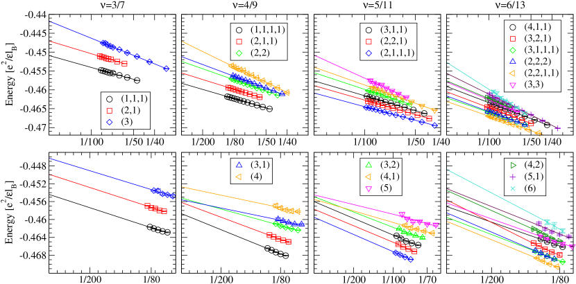
Figure 2: [Color online] Energy per particle for the novel incompressible composite fermion ground state wave functions for the sequence $\tilde{\nu}=m/(2pm+1)$. The states are denoted by $(l_{1},l_{2},l_{3},l_{4})$, explained in the text. The upper panels are for the $n=0$ Landau level, and the lower panels for the $|n|=1$ Landau level. The energies are given in units of $e^{2}/\epsilon l_{B}$, where $l_{B}=\sqrt{\hbar c/eB}$ is the magnetic length. The thermodynamic limits of the the ground state energies are given in Table 5.

$\tilde{\nu}$	State	Energy $n=0$	Energy $n=1$	$\hbar\omega_{c}^{\ast}/N$
$\frac{3}{7}$	(3)	-0.44178(8)	-0.4463(14)	1
	(2,1)	-0.44704(15)	-0.4499(7)	1/3
	(1,1,1)	-0.45090(3)	-0.4544(4)	0
$\frac{4}{9}$	(4)	-0.4471(2)	-0.4527(15)	3/2
	(3,1)	-0.4512(1)	-0.4556(12)	3/4
	(2,2)	-0.45244(9)	-0.4552(6)	1/2
	(2,1,1)	-0.45552(12)	-0.4562(7)	1/4
	(1,1,1,1)	-0.45825(5)	-0.4587(5)	0
$\frac{5}{11}$	(5)	-0.4508(4)	-0.4545(9)	2
	(4,1)	-0.45399(11)	-0.4555(7)	6/5
	(3,2)	-0.45544(16)	-0.4549(2)	4/5
	(3,1,1)	-0.45762(8)	-0.4560(6)	3/5
	(2,2,1)	-0.45888(7)	-0.4577(8)	2/5
	(2,1,1,1)	-0.46084(5)	-0.4595(9)	1/5
$\frac{6}{13}$	(6)	-0.4527(4)	-0.4488(19)	5/2
	(5,1)	-0.4556(1)	-0.4531(14)	5/3
	(4,2)	-0.4576(4)	-0.4535(7)	7/6
	(3,3)	-0.4579(2)	-0.4563(6)	1
	(4,1,1)	-0.4591(1)	-0.4571(13)	1
	(3,2,1)	-0.4605(1)	-0.4556(8)	2/3
	(2,2,2)	-0.46161(9)	-0.4585(9)	1/2
	(3,1,1,1)	-0.4621(1)	-0.4595(6)	1/2
	(2,2,1,1)	-0.46308(4)	-0.4604(7)	1/3

Table 5: Energy per particle for incompressible composite fermion ground state candidates of different SU(4) symmetries at $\tilde{\nu}=\frac{m}{2m+1}$, corresponding to the integral quantum Hall effect of ²CFs. For each fraction $\tilde{\nu}$ the states are listed in decreasing order of energy. The last column gives the CF kinetic energy ($\hbar\omega_{c}^{*}$) per particle in the thermodynamic limit, measured relative to the energy of the lowest $\Lambda$ level.

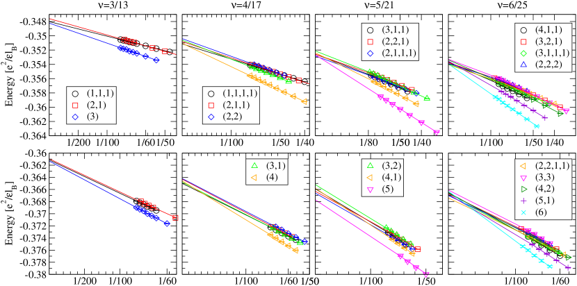
Figure 3: [Color online] Same as in Fig. 2, but for the sequence $\tilde{\nu}=m/(4m+1)$, corresponding to the integral quantum Hall effect of ⁴CFs. The thermodynamic limits of the the ground state energies are given in Table 6.

$\tilde{\nu}$	State	Energy $n=0$	Energy $n=1$	$\hbar\omega_{c}^{\ast}/N$
$\frac{3}{13}$	(2,1)	-0.34759(4)	-0.36094(17)	1/3
	(1,1,1)	-0.34801(3)	-0.36112(17)	0
	(3)	-0.34822(12)	-0.36131(29)	1
$\frac{4}{17}$	(2,2)	-0.35040(8)	-0.3642(2)	1/2
	(3,1)	-0.35062(7)	-0.3648(2)	3/4
	(2,1,1)	-0.35081(3)	-0.3643(2)	1/4
	(4)	-0.35106(5)	-0.3646(3)	3/2
	(1,1,1,1)	-0.35114(3)	-0.3650(1)	0
$\frac{5}{21}$	(3,2)	-0.35212(5)	-0.3652(3)	4/5
	(4,1)	-0.35238(9)	-0.3658(4)	6/5
	(3,1,1)	-0.35257(5)	-0.3659(3)	3/5
	(2,2,1)	-0.35257(5)	-0.3663(1)	2/5
	(5)	-0.35266(10)	-0.3677(3)	2
	(2,1,1,1)	-0.35283(6)	-0.3666(3)	1/5
$\frac{6}{25}$	(3,3)	-0.35328(2)	-0.3661(2)	1
	(4,2)	-0.35337(6)	-0.3666(2)	7/6
	(5,1)	-0.35354(9)	-0.3668(4)	5/3
	(4,1,1)	-0.35366(5)	-0.3665(1)	1
	(3,2,1)	-0.35375(3)	-0.3667(1)	2/3
	(2,2,2)	-0.35387(7)	-0.3670(2)	1/2
	(3,1,1,1)	-0.35393(3)	-0.3669(1)	1/2
	(6)	-0.35394(18)	-0.3663(6)	5/2
	(2,2,1,1)	-0.35405(4)	-0.3674(2)	1/3

Table 6: Same as in Table 5 for $\tilde{\nu}=\frac{m}{4m+1}$, corresponding to the integral quantum Hall effect of ⁴CFs. Energies per particle for incompressible composite fermion ground state candidates with different SU(4) symmetries are shown in decreasing order. For each fraction $\tilde{\nu}$ the states are in decreasing order of energy.

VI Quantum phase transitions

Either the Zeeman energy $E_{Z}^{S}=q\mu_{B}\vec{B}\cdot\vec{S}$, or the pseudo-Zeeman energy $E_{Z}^{P}=\Delta P_{z}$, or both, will break the SU(4) symmetry. Assuming the symmetry-breaking fields are weak, the effect will be to select the most favorable member of the ground state multiplet. (Notice that $P_{z}$, $S_{z}$, as well as the third member $E_{00}$ of the Abelian subalgebra of SU(4) generators, commute with the Hamiltonian of Eq. (1) in the SU(4) symmetric $\Delta\to 0,g\to 0$ limit.) Slightly stronger fields may drive zero-temperature phase transitions between the possible CF ground states at a fixed filling factor. It is convenient to change to new quantum numbers $S^{\prime}_{z},P^{\prime}_{z}$ by

$$\begin{pmatrix}S^{\prime}_{z}\\ P^{\prime}_{z}\end{pmatrix}=U\begin{pmatrix}S_{z}\\ P_{z}\end{pmatrix},$$ (19)

with a unitary $U$ to eliminate one kind of Zeeman energy. Choosing

$$U=\frac{1}{\sqrt{1+\lambda^{2}}}\begin{pmatrix}1&\lambda\\ -\lambda&1\end{pmatrix},$$ (20)

with $\lambda=E^{P}_{Z}/E^{S}_{Z}$ yields

$${E_{Z}^{S}}^{\prime} = \frac{1}{\sqrt{1+\lambda^{2}}}E^{S}_{Z}+\frac{\lambda}{\sqrt{1+\lambda^{2}}}E^{P}_{Z},$$

$${E_{Z}^{P}}^{\prime} = 0.$$

The phase transitions driven by the effective ${E_{Z}^{S}}^{\prime}$ are given in Table 7. Here we assume a sufficiently weak field that does not mix the low-lying states, but only selects the most favorable member of the ground state multiplet. In state $(l_{1},l_{2},l_{3},l_{4})$ the with $l_{i}\geq l_{i+1}$, this means filling $l_{1}+l_{2}$ $\Lambda$ levels of the favorable $S^{\prime}$ spin, and $l_{3}+l_{4}$ levels of the unfavorable $S^{\prime}$ spin. This results in an effective Zeeman energy difference per particle. Notice that no value of $E^{P}_{Z}$ and $E^{S}_{Z}$ will drive the system at $\tilde{\nu}=m/(2pm+1)$ to a completely antisymmetric orbital state $(m)$. This is a consequence of our freedom to choose a basis $P^{\prime}_{z},S^{\prime}_{z}$ in the Cartan subalgebra of SU(4) (Eq. (19)), which eliminates one kind of Zeeman energy; the states where the two unfavorable bands of the $S^{\prime}$ spin are emptied will already have the lowest possible effective Zeeman energy ${E_{Z}^{S}}^{\prime}$.

Tilting the magnetic field is often used as a means to tune the effective Zeeman energy. Unlike in GaAs/AlGaAs heterostructures, the in-plane megnetic field is unlikely to change the single-particle states in any significant manner, because the transverse thickness of the two dimensional electron system is graphene ($\sim 2$Å) is much smaller than the typical magnetic lengths ($\sim$100Å). The most favorable parameter space for the observation of these transitions occurs for very low values of the dielectric constant $\epsilon$ and the sublattice asymmetry $\Delta$. The value of $\epsilon$ depends on the interaction with the substrate on which the graphene sheet is placed.

$\tilde{\nu}$	Transition	$\left(\frac{{E_{Z}^{S}}^{\prime}}{e^{2}/\epsilon l_{B}}\right)_{c}$	Change of $\langle S^{\prime}\rangle$
$\frac{3}{7}$	$(1,1,1)\to(2,1)$	0.0116(6)	$\frac{1}{6}\to\frac{1}{2}$
$\frac{4}{9}$	$(1,1,1,1)\to(2,1,1)$	0.0109(7)	$0\to\frac{1}{4}$
	$(2,1,1)\to(2,2)$	0.0123(8)	$\frac{1}{4}\to\frac{1}{2}$
$\frac{5}{11}$	$(2,1,1,1)\to(2,2,1)$	0.0098(6)	$\frac{1}{10}\to\frac{3}{10}$
	$(2,2,1)\to(3,2)$	0.0172(8)	$\frac{3}{10}\to\frac{1}{2}$
$\frac{6}{13}$	$(2,2,1,1)\to(3,2,1)$	0.0076(5)	$\frac{1}{6}\to\frac{1}{3}$
	$(3,2,1)\to(3,3)$	0.016(2)	$\frac{1}{3}\to\frac{1}{2}$

Table 7: Zero temperature phase transitions driven by the effective Zeeman energy in the $n=0$ Landau level. The last column gives the expectation value of the transformed spin $S^{\prime}$ (Eq. (19)), which coincides with the ordinary spin in the case of perfect sublattice symmetry ($\Delta=0$). The quantity $\left({{E_{Z}^{S}}^{\prime}}/{(e^{2}/\epsilon l_{B})}\right)_{c}$ give the value of the parameter where the transition is predicted to take place.

VII Conclusion

We have used a combination of exact diagonalization and the CF theory to identify a large range of possible FQHE states in graphene allowed by SU(4) symmetry, and shown that new states, which have no analog in GaAs, can occur at filling factors $\tilde{\nu}=\frac{m}{2pm\pm 1}$ for $m\geq 3$ in the $|n|=0$ and $|n|=1$ Landau levels of graphene. For ²CFs, the ground states are those for which the composite fermion kinetic energy is minimum; these states spread out maximally in SU(4) spin space. For ⁴CFs the fully polarized ground state wins, with the exception of $\tilde{\nu}=\frac{4}{17}$, where very compact SU(4) singlet structures are possible. We have also estimated parameter regimes where these states should occur; zero temperature phase transitions can be driven by variation of an effective Zeeman energy that accounts for the combined effect of the Zeeman energy and the sublattice symmetry breaking field. At $\tilde{\nu}=\frac{1}{3}$ we found SU(4) skyrmions to be the lowest energy charged excitations.

We thank the High Performance Computing (HPC) group at Penn State University ASET (Academic Services and Emerging Technologies) for assistance and computing time on the Lion-XO cluster. Partial support of this research by the National Science Foundation under grant No. DMR-0240458 is gratefully acknowledged.

References

- (1) K. von Klitzing, G. Dorda, and M. Pepper, Phys. Rev. Lett. 45, 494 (1980).
- (2) K. S. Novoselov et al., Nature 438, 197 (2005); Y. Zhang et al., Nature 438, 201 (2005).
- (3) G. W. Semenoff, Phys. Rev. Lett. 53, 2449 (1984); F. D. M. Haldane, Phys. Rev. Lett. 61, 2015 (1988).
- (4) Y. Zhang et al., Phys. Rev. Lett. 96, 136806 (2006).
- (5) K. Yang, S. Das Sarma, A. H. MacDonald, Phys. Rev. B 74, 075423 (2006).
- (6) S. L. Sondhi,A. Karlhede, S. A. Kivelson, and E. H. Rezayi, Phys. Rev. B 47, 16419 (1993); S. E. Barrett, G. Dabbagh, L. N. Pfeiffer, K. W. West, and R. Tycko, Phys. Rev. Lett. 74, 5112 (1995); A. Schmeller, J. P. Eisenstein, L. N. Pfeiffer, and K. W. West, Phys. Rev. Lett. 75, 4290 (1995); E. H. Aifer, B. B. Goldberg, and D. A. Broido, Phys. Rev. Lett. 76, 680 (1996).
- (7) C. Tőke, P. E. Lammert, V. H. Crespi, and J. K. Jain, Phys. Rev. B 74, 235417 (2006).
- (8) D. C. Tsui, H. L. Stormer, and A. C. Gossard, Phys. Rev. Lett. 48, 1559 (1982).
- (9) V. M. Apalkov and T. Chakraborty, Phys. Rev. Lett. 97, 126801 (2006); M. O. Goerbig, R. Moessner, and B. Douçot, Phys. Rev. B 74, 161407(R) (2006).
- (10) X. G. Wu, G. Dev, and J. K. Jain, Phys. Rev. Lett. 71, 153 (1993).
- (11) K. Park and J. K. Jain, K. Park and J.K. Jain, Phys. Rev. Lett. 80, 4237 (1998); Solid State Comm. 119, 291 (2001).
- (12) F. D. M. Haldane, Phys. Rev. Lett. 51, 605 (1983); also in The Quantum Hall Effect, edited by S.M. Girvin (Springer, New York, 1987).
- (13) J. K. Jain, Phys. Rev. Lett. 63, 199 (1989); J. K. Jain, Composite Fermions, Camridge University Press (2007).
- (14) D. P. DiVincenzo and E. J. Mele, Phys. Rev. B 29, 1685 (1984); N. H. Shon and T. Ando, J. Phys. Soc. Jpn. 67, 2421 (1998).
- (15) G. Fano, F. Ortolani, and E. Colombo, Phys. Rev. B 34, 2670 (1986).
- (16) P. A. M. Dirac, Proc. R. Soc. London, Ser. A 133, 60 (1931).
- (17) T. T. Wu and C. N. Yang, Nucl. Phys. B 107, 365 (1976).
- (18) J. K. Jain and R. K. Kamilla, Int. J. Mod. Phys. B11, 2621 (1997); Phys. Rev. B 55, R4895 (1997).
- (19) W. Ludwig and C. Falter, Symmetries in Physics (Springer, 2nd ed., 1995).
- (20) M. Hamermesh, Group Theory and its Application to Physical Problems (Addison-Wesley, Reading MA, 1962).
- (21) C. Quesne, J. Math. Phys. 17, 1452 (1976).
- (22) K. T. Hecht and S. C. Pang, J. Math. Phys. 10, 1571 (1968).
- (23) R.K. Kamilla, X.G. Wu, and J.K. Jain, Solid State Commun. 99, 289 (1996); A. Wójs and J. J. Quinn, Phys. Rev. B 66, 045323 (2002); D. R. Leadley et al., Phys. Rev. Lett. 79, 4246 (1997); A. F. Dethlefsen, R. J. Haug, K. Výborný, and O. Čertík, Phys. Rev. B 74, 195324 (2006).
- (24) C. Tőke, M. R. Peterson, G. S. Jeon, and J. K. Jain, Phys. Rev. B 72, 125315 (2005).
- (25) K. Park et al., Phys. Rev. B 58, R10167 (1998); S.-Y. Lee, V.W. Scarola, and J.K. Jain, Phys. Rev. Lett. 87, 256803 (2001).
- (26) K. Park and J.K. Jain, Phys. Rev. Lett. 83, 5543 (1999).
- (27) G. Möller and S. H. Simon, Phys. Rev. B 72, 045344 (2005).