Magnetic-field symmetries of mesoscopic nonlinear conductance

Abstract

We examine contributions to the dc-current of mesoscopic samples which are non-linear in applied voltage. In the presence of a magnetic field, the current can be decomposed into components which are odd (antisymmetric) and even (symmetric) under flux reversal. For a two-terminal chaotic cavity, these components turn out to be very sensitive to the strength of the Coulomb interaction and the asymmetry of the contact conductances. For both two- and multi-terminal quantum dots we discuss correlations of current non-linearity in voltage measured at different magnetic fields and temperatures.

I Introduction

Symmetries are of fundamental interest in all fields of physics. In linear irreversible transport the Onsager-Casimir Onsager symmetry relations are important since they relate different transport coefficients. Here we are concerned with electron transport on the mesoscopic scale. This scale emerges when the distance carriers can travel without losing their phase coherence becomes comparable to the dimensions of the sample. It has long been understood that the Onsager-Casimir relations are not restricted to the macroscopic domain but extend to linear transport on the mesoscopic scale. For the linear conductance $G_{\alpha\beta}=dI_{\alpha}/dV_{\beta}$ Onsager-Casimir implies that under field reversal we have the symmetry $G_{\alpha\beta}(\Phi)=G_{\beta\alpha}(-\Phi)$. An important condition is that voltages are measured at contacts which are sufficiently large such that they can effectively be considered as equilibrium electron reservoirsMarkus_1986 .

Since symmetries are important it is crucial to understand their limit of validity. Are Onsager-Casimir relations strictly valid only in the linear transport regime? What could cause their breakdown? Is it possible to quantify and measure the departure from symmetry? In this work we report recent theoretical and experimental progress on these questions using as an example electron transport through a chaotic quantum dot. We extend earlier discussions to correlations of current non-linearity in voltage measured at different magnetic fields and temperatures. Interestingly, as we will now discuss, these questions are related to the role Coulomb interactions play in non-linear transport.

In the mesoscopic regime the linear conductance depends on quantum interference meso and depends on Coulomb interactions. A change in the Hartree potential is similar to a small change in the shape of the sample or in its impurity configuration and thus needs no separate discussion. In contrast Hartree-Fock terms AA can modify the conductance significantly. A well known example of such an interaction effect is the physics of Coulomb blockade which becomes relevant at low temperatures if the contacts are pinched-off. However, if the conductance of the quantum dot with ballistic contacts is large, $G=(e^{2}/h)g\gg e^{2}/h$, Fock terms give only a small relative correction $\lesssim 1/g$ to sample-specific quantum fluctuations. In such open dots weak localization corrections (WL) or universal conductance fluctuations (UCF) remain universal at low temperatures. In particular, Coulomb interactions do not affect WL and just slightly ($\lesssim 1/g$) modify UCF only at elevated temperatures BLF . Since these effects due to many-body physics in open quantum dots appear only as small corrections to non-interacting theory, one could conclude that Coulomb interaction effects are unimportant.

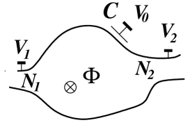
Figure 1: Quantum dot with magnetic flux $\Phi$ and dc bias voltages $V_{1,2}$ at the contacts and $V_{0}$ at the gates with capacitance $C$.

However, Coulomb interactions play a much more important role in non-linear transport. Experimentally transport is characterized by the full conductance $I/V$ rather then the differential conductance, $dI/dV\neq I/V$. In particular, here we are interested in $(1/2)\partial^{2}I/\partial V^{2}$ (at $V=0$) which we call the second-order non-linear conductance or simply the non-linear conductance. In this regime it is the Coulomb interaction that breaks the symmetry of the Onsager-Casismir relations. Conversely, measurement of transport non-linearity provides a tool to determine interactions.

Initial discussions of non-linear dc- transport AK ; KL and the rectification of an ac-applied voltage FK in mesoscopic samples were addressed without taking interaction effects into account. Interestingly, inclusion of Coulomb interaction does not only modify these phenomena but also leads to a qualitatively new effect: namely, even in a two terminal conductor it is possible to have a component to the current which is odd in magnetic field $I(\Phi)\neq I(-\Phi)$. In generic mesoscopic conductors, in chaotic cavities (quantum dots) and in metallic diffusive conductors this effect vanishes when an average is taken over many samples of slightly different geometry or impurity configuration (mesoscopic averaging) SB ; SZ . Thus in generic mesoscopic conductors this is purely a quantum effect.

Sánches and Büttiker investigated the effect of interactions on current-voltage characteristic of open chaotic (ballistic or diffusive) cavities, see Fig. 1, in the presence of a magnetic flux $\Phi$ comparable to a flux quantum $\Phi_{0}=eh/c$. SB They found the dependence of the fluctuation of the antisymmetric component on the interaction strength and the dependence on the number of ballistic channels transmitted through the contacts of the cavity. Spivak and Zyusin explored this asymmetry at small fields, $\Phi\ll\Phi_{0}$, and weak interactions in open diffusive samples SZ . Under these conditions the asymmetric fluctuations are linear in flux and interaction strength. Polianski and Büttiker PB present a theory which describes the entire crossover from the regime of low magnetic fields to the regime considered in Ref. SB, in which the flux through the sample is comparable to a flux quantum $\Phi_{0}$.

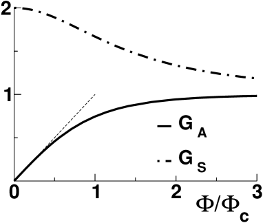
Figure 2: Normalized fluctuation of the (anti)symmetric nonlinear conductance $({\mathcal{G}}_{a}){\mathcal{G}}_{s}$ as a function of flux $\Phi/\Phi_{c},\Phi_{c}\ll\Phi_{0}$ for strongly interacting dot with symmetric contacts, from PB .

The experiments measured field asymmetry in a wide range of structures: in nanotubes wei , ballistic billiards marlow , ballistic quantum dots Zumbuhl , ballistic ensslin and diffusive Bouchiat Aharonov-Bohm rings. This motivated further research on non-linear quantum BS ; Tsvelik and classical AG effects. The experiment by Zumbühl et al.Zumbuhl investigated this asymmetry in chaotic ballistic dots at very low voltages. The experiment demonstrated that the asymmetry vanishes on average and depends linearly on flux at sufficiently small fields. The experiment also investigates the dependence of the asymmetry on the number of channels in the contacts of the sample. Some experimental results, especially, the magnitude of the asymmetry, if four or more channels are open, agree well with existing theories SB ; SZ ; PB . A more detailed investigation of the dependence on various external parameters is still necessary.

Theoretically Ref. PB, considers fluctuations of both anti-symmetric and symmetric component of non-linear conductance

$$\binom{{\mathcal{G}}_{s}(\Phi)}{{\mathcal{G}}_{a}(\Phi)}\equiv\frac{h}{4e^{2}}\left.\frac{\partial^{2}}{\partial V^{2}}\left(\frac{I(\Phi)\pm I(-\Phi)}{2}\right)\right|_{V\to 0}$$ (1)

through a 2-terminal quantum dot with arbitrary interaction strength, flux, temperature and dephasing PB . The fluctuations (square root of the variance) of these two quantities are shown in Fig. 2 as a function of the flux applied to the cavity. Interestingly, similarly to linear transport (see references in Beenakker ), the crossover of ${\mathcal{G}}_{a}$ and ${\mathcal{G}}_{s}$ from low to high magnetic fields is shown to depend on the flux $\Phi_{c}\ll\Phi_{0}$ and not on the flux quantum $\Phi_{0}$ characteristic for open diffusive samples. Since the dot is essentially zero-dimensional, the dwell time $\tau_{\rm d}$ an electron spends inside is much larger then the ergodic time $\tau_{\rm erg}$ necessary to explore the phase space of the dot. Therefore an electronic trajectory gains a flux $\sim\Phi_{0}$ during $\tau_{\rm d}/\tau_{\rm erg}\gg 1$ random explorations of the dot already at $\Phi\sim\Phi_{0}/\sqrt{\tau_{\rm d}/\tau_{\rm erg}}\ll\Phi_{0}$. Fluctuations of ${\mathcal{G}}_{a},{\mathcal{G}}_{s}$ occur on the background of an ensemble averaged anti-symettrized $\langle{\mathcal{G}}_{a}\rangle=0$ and symmetrized $\langle{\mathcal{G}}_{s}\rangle=0$ non-linear conductance. The magnitude of these fluctuations as a function of flux $\Phi/\Phi_{c}$ is shown in Fig. 2 for the limit of strongly interacting dot with symmetric contacts (corresponding to the experiment Zumbuhl ).

However, if either the Coulomb interaction is not very strong or ballistic contacts are unequal, $N_{1}\neq N_{2}$ on Fig. 1, the field-asymmetry of the non-linear signal may be strongly reduced compared to strongly interacting symmetric set-up. In practice, to observe a strong violation of Onsager relations wei ; marlow ; Zumbuhl ; ensslin ; Bouchiat one might want to consider not the amplitude of ${\mathcal{G}}_{a}$, but rather the relative asymmetry in the signal, denoted here ${{\mathcal{A}}}={\mathcal{G}}_{a}/{\mathcal{G}}_{s}$. Below we discuss the optimal regime to maximize this ratio. We find how magnetic field and temperature affect fluctuations of this asymmetry parameter and find the contact asymmetry that maximizes ${\mathcal{A}}$. For sufficiently strong interaction, symmetric contacts turn out to be the optimal regime. Surprisingly, however, if the interactions are not very strong an asymmetric set-up, $N_{1}\neq N_{2}$, is more advantageous.

Since both field-components ${\mathcal{G}}_{a},{\mathcal{G}}_{s}$ were recently explored experimentally Zumbuhl ; Bouchiat , we consider the statistics of ${\mathcal{G}}_{a}$ and ${\mathcal{G}}_{s}$ and their correlations for arbitrary interactions. Particularly, in the non-interacting limit we find an universal relation between UCF and fluctuations of ${\mathcal{G}}_{s}$, independent of temperature and applied field. In view of a multi-terminal experiment ensslin , we generalize our treatment of an asymmetric component ${\mathcal{G}}_{a}$ to a multi-terminal dot and consider non-linearity not only with respect to a contact, but also to the gate voltage. In the end we discuss interaction effects in linear vs. non-linear transport, applicability of existing theories to experimental data and provide a formula for fluctuations of the asymmetry ${\mathcal{A}}$ in the experimental regime of Ref. Zumbuhl, .

The paper is organized as follows: Sec. II describes the model and the basic steps of our approach. We present our results in Sec. III and discuss them in Sec. IV.

II Model

The 2D chaotic quantum dot, see Fig. 1, is biased with dc voltages $V_{\alpha},\alpha=1,...,M$ at contacts with $N_{\alpha}$ ballistic channels, and by the voltage $V_{0}$ at the gates with capacitance $C$. Chaos in the dot is either due to diffusive scattering off impurities, when the mean free path is smaller then the size of the dot, $l\ll L$, or due to the irregular shape of a ballistic dot with chaotic classical dynamics, $l\gg L$. The dot is in the universal regime Beenakker ; ABG , when the Thouless energy $E_{\rm T}=\hbar/\tau_{\rm erg}$ is the largest energy-scale in the problem. Typically $E_{\rm Th}\sim\hbar\mbox{ min }\{lv_{\rm F}/L^{2},v_{\rm F}/L\}$, see the review Beenakker for details. The mean level spacing (per spin direction) $\Delta=2\pi\hbar^{2}/(m^{*}\mbox{ Area})$ and the number of conducting channels $N$ together define the dwell time $\tau_{\rm d}=h/(N\Delta)\gg\tau_{\rm erg}$ which an electron typically spends inside the dot.

Scattering is assumed spin-independent and this spin degeneracy is explicitly accounted for by the factor $\nu_{s}$. The number $N$ of ballistic (orbital) channels in the contacts is assumed to be large, $N\gg 1$, so that the problem can be considered analytically. We use Random Matrix Theory (RMT) for the energy-dependent scattering matrix ${\mathcal{S}}(\varepsilon)$ and refer reader to reviews Beenakker ; ABG for details of RMT and its relation to Green function technique. The diagrammatic technique based on small parameter $1/N\ll 1$ expansion are given in diagram for energy-independent scattering matrix ${\mathcal{S}}$ and in iop for energy-dependent ${\mathcal{S}}(\varepsilon)$. We also require that the transport is only weakly nonlinear and refer to KL ; LBM for a discussion of highly nonlinear transport in mesoscopic samples. Here we assume that $eV\ll N\Delta$ and treat the $I-V$ nonlinearity only to order $(eV)^{2}$, see Eq. (1). The energy dependence of the ${\mathcal{S}}$-matrix allows us to consider non-zero temperatures $T\ll E_{\rm Th}$, and for convenience we normalize it to dimensionless parameter $t\equiv 2\pi T/(N\Delta)$.

The magnetic field appears via the total flux $\Phi$ through the dot. For simplicity the dot is assumed here to be (nearly) circular with radius $L$. As discussed in Sec. I, the relevant flux-scale for the dot in the diffusive and the ballistic regime is $\Phi_{c}\ll\Phi_{0}$ Beenakker ; PB . Therefore for convenience we normalize magnetic flux $\Phi$ through the dot to dimensionless flux $\phi$ as follows:

$$\phi=\frac{\Phi}{\Phi_{0}}\frac{\sqrt{\tau_{\rm d}v_{F}l}}{2L}.$$ (2)

To describe the crossover from the diffusive to the ballistic regime we use the substitute $l\to\pi L/4$ according to Adam (the numerical factor given in FrahmPichard ; Beenakker is not correct). The importance of crossover is evident if one notices that much of the data Zumbuhl taken pertains to this intermediate regime.

The geometrical capacitance $C$ of the dot can be defined, e.g. in the constant interaction model in the Hamiltonian approach ABG from the solution of electrostatic problem, if the shape of the dot is known exactly and all nearby conductors are taken into account. Usually such an exact solution is not available, but this capacitance can be estimated either as $C\sim\epsilon L$ for an ungated sample or as $C\sim\epsilon L^{2}/d$ for macroscopic gates separated by a distance $d$ from the dot. (Here $\epsilon$ is the dielectric constant). This capacitance defines the strength of the Coulomb interaction, and electronic repulsion is referred here as ’strong’ if a typical charging energy is large compared to the level spacing, $e^{2}/C\gg\Delta$.

For strong screening in the dot, $r_{s}=(k_{\rm F}a_{B})^{-1}=e^{2}/(\epsilon\hbar v_{\rm F})\lesssim 1$, an RPA treatment of Coulomb interactions is sufficient. Furthermore, for large dots, $L\gg a_{B}$, only the long distance screening is relevant. As a consequence, electrons with kinetic energy $\varepsilon$ have a well-defined electro-chemical potential $\tilde{\varepsilon}_{\alpha}=\varepsilon-eV_{\alpha}$ in the contact $\alpha$ and $\tilde{\varepsilon}=\varepsilon-eU(\vec{r})$ in the dot. For a quantum dot large compared to the Bohr radius but still so small that its dimensionless conductance, $g_{\rm dot}=E_{\rm Th}/\Delta$ is much larger then conductance of the contacts, $g_{\rm dot}\gg N$, the potential can be taken uniform (’zero-mode approximation’)ABG . The leading interactions are then present in the form of a Hartree electrical potential $U$ which shifts the bottom of the energy band in the dot, see Fig. 3 and therefore modifies the ${\mathcal{S}}$-matrix.

Therefore, transport depends on the Fermi-distributions $f(\tilde{\varepsilon}_{\alpha})$ and the scattering matrix ${\mathcal{S}}(\tilde{\varepsilon})$. The current in contact $\alpha$ is $I_{\alpha}=\int d\varepsilon I_{\alpha}(\varepsilon)$ and for $eV\ll N\Delta$ the spectral current $I_{\alpha}(\varepsilon)$ can be expanded in powers of $eV$:

$$I_{\alpha}(\varepsilon)=\frac{\nu_{s}e^{2}}{h}\sum_{\delta=1}^{M}f(\tilde{\varepsilon}_{\delta})\mbox{tr}\,\left[{1\!\!1}_{\alpha}\delta_{\alpha\delta}-{1\!\!1}_{\delta}{\mathcal{S}}^{\dagger}(\tilde{\varepsilon}){1\!\!1}_{\alpha}{\mathcal{S}}(\tilde{\varepsilon})\right]$$

$$\approx\frac{\nu_{s}e^{2}}{h}\sum_{\beta}g_{\alpha\beta}(\varepsilon)V_{\beta}+\frac{\nu_{s}e^{3}}{h}\sum_{\beta\gamma}g_{\alpha\beta\gamma}(\varepsilon)V_{\beta}V_{\gamma}.$$ (3)

In Eq. (II) the total current $I_{\alpha}$ is expressed in terms of the dimensionless linear conductance at energy $\varepsilon$, $g_{\alpha\beta}(\varepsilon)=\mbox{tr}\,({1\!\!1}_{\alpha}\delta_{\alpha\beta}-{1\!\!1}_{\beta}{\mathcal{S}}^{\dagger}(\varepsilon){1\!\!1}_{\alpha}{\mathcal{S}}(\varepsilon))$ and the nonlinear conductance (measured in units of inverse energy) $g_{\alpha\beta\gamma}(\varepsilon)=(h/2\nu_{s}e^{3})\partial^{2}I_{\alpha}(\varepsilon)/\partial V_{\beta}\partial V_{\gamma}$, which depends on the potential $U$. To this accuracy $U$ needs to be known only up to the first order derivatives, the characteristic potentials $u_{\alpha}=\partial U/\partial V_{\alpha}$ mb93 ; ChristenButtiker ; Christen97 . The characteristic potentials $u_{\alpha}$ are found self-consistently RPA from current conservation and gauge-invariance requirements. The dc limit $\omega\to 0$ of an ac-result iopBP reads

$$u_{\alpha} = \frac{-\int d\varepsilon f^{\prime}(\varepsilon)\mbox{tr}\,{\mathcal{S}}^{\dagger}\partial_{\varepsilon}{\mathcal{S}}{1\!\!1}_{\alpha}}{2\pi iC/\nu_{s}e^{2}-\int d\varepsilon f^{\prime}(\varepsilon)\mbox{tr}\,{\mathcal{S}}^{\dagger}\partial_{\varepsilon}{\mathcal{S}}},$$ (4)

$$u_{0} = \frac{2\pi iC/\nu_{s}e^{2}}{2\pi iC/\nu_{s}e^{2}-\int d\varepsilon f^{\prime}(\varepsilon)\mbox{tr}\,{\mathcal{S}}^{\dagger}\partial_{\varepsilon}{\mathcal{S}}}=1-\sum_{\alpha=1}^{M}u_{\alpha}.$$ (5)

We point out that this self-consistent treatment of Coulomb interactions has certain limitations. Remaining in a single-particle picture of scattering, we neglect many-body effects. We consider here a dot with multi-channel ballistic contacts, $N\gg 1$ when scattered wave-packets are delocalized. Then the effects of Fock terms are small $\lesssim 1/N$ compared to that of Hartree self-consistent potential BLF ; VA .

The sample-specific fluctuations of $u_{\alpha}$ are dependent on magnetic flux $\phi$, and determine the field-asymmetry of the non-linear conductance. These derivatives are used to express the conductances $g_{\alpha\beta\gamma}(\varepsilon)$:

$$g_{\alpha\beta\gamma}(\varepsilon)=\frac{-f^{\prime}(\varepsilon)}{2}\left(\delta_{\beta\gamma}g^{\prime}_{\alpha\beta}-u_{\beta}g^{\prime}_{\alpha\gamma}-u_{\gamma}g^{\prime}_{\alpha\beta}\right),$$ (6)

where the prime stands for energy derivative. Transport coefficients in general depend on magnetic field due to sensitivity of the matrix $\mathcal{S}$ to magnetic field. For example, field inversion transposes the scattering matrix ${\mathcal{S}}(\phi)={\mathcal{S}}^{\rm T}(-\phi)$. The response to the gate voltage remains invariant under such inversion, $u_{0}(-\phi)=u_{0}(\phi)$, but the response to the voltage at the contacts is asymmetric, $u_{\alpha}(\phi)\neq u_{\alpha}(-\phi)$.

We point out that this $\phi$-sensitivity of electrostatic potential $U(\vec{r},\phi)$, which locally shifts the bottom of the energy band, is a general feature of coherent systems. In the high-field limit of Quantum Hall bar a voltage applied to one of the contacts changes the electric potential only in the outgoing edge, but not in the incoming. The field inversion reverses the direction of edge channels, so the same voltage induces a potential on the opposite edge, $U(\vec{r},\Phi)\neq U(\vec{r},-\Phi)$. The magnetic field asymmetry in an edge state geometry with a Coulomb blockaded impurity is the subject of Ref. SB_Coulomb, . Even at the small fields, $\Phi\lesssim\Phi_{0}$, of interest here, the potential $U(\vec{r})$ remains field-sensitive, although the field effect is not as drastic as in the edge state geometries mentioned above.

Since the dot is a good conductor compared to contacts, $E_{\rm Th}/\Delta\gg N$, the voltage drops mainly over the ballistic contacts and remains uniform inside the dot. This is qualitatively sketched by the bold curve in Fig. 3 (dashed curves correspond to the potential for channels reflected by the ballistic constriction). Therefore in a quantum dot we deal with a uniform potential $U(\vec{r},\phi)=U(\phi)$. This is very different from an open diffusive sample, where $\tau_{\rm erg}\sim\tau_{\rm d}$ and the voltage drops gradually.

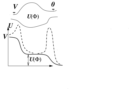
Figure 3: Electric potential $U(x)$ shifts the bottom of the energy band. Bold curve corresponds to open channels and dashed (dot-dashed) correspond to (classically) reflected channels. Potential $U$ varies only in the contact regions and remains constant inside the dot.

Classically the voltage through such a conducting nod is divided according to the widths of the contacts, $u_{{\rm cl}\,\alpha}=\partial U_{\rm cl}/\partial V_{\alpha}=N_{\alpha}/N\sim 1$, is insensitive to magnetic field. However, since the phases of scattering amplitudes between different channels are modified by the magnetic field, a field-sensitive and sample-specific correction $\delta u_{\alpha}=u_{\alpha}-u_{{\rm cl}\,\alpha}\sim 1/N$ appears. Although at such small fields it is small compared to classical the value, its asymmetry with respect to magnetic field $\delta u_{\alpha}(\phi)\neq\delta u_{\alpha}(-\phi)$ leads to the asymmetry in the current-voltage characteristic, and more specifically in the non-linear conductance $g_{\alpha\beta\gamma}(\phi)\neq g_{\alpha\beta\gamma}(-\phi)$. Below, these (anti-)symmetric components of conductance, $({\mathcal{G}}_{a}){\mathcal{G}}_{s}$,

$$\binom{{\mathcal{G}}_{s}}{{\mathcal{G}}_{a}}_{\alpha\beta\gamma}\equiv\frac{1}{2}\int d\varepsilon\left(g_{\alpha\beta\gamma}(\varepsilon,\phi)\pm g_{\alpha\beta\gamma}(\varepsilon,-\phi)\right),$$ (7)

are investigated in detail (for a 2-terminal dot Eq. (7) corresponds to Eq. (1) for $\alpha=\beta=\gamma=1$).

III Results

We group our results into two subsections. First in Sec. III.1 we consider two-terminal dots and discuss properties of the ensemble averaged non-linear conductances ${\mathcal{G}}_{a},{\mathcal{G}}_{s}$. Since the field-asymmetry of the measured signal is characterized by the relative strength of the components introduced in Eq. (7), we start by considering fluctuations and correlations of ${\mathcal{A}}={\mathcal{G}}_{a}/{\mathcal{G}}_{s}$, and discuss the dependence of ${\mathcal{A}},{\mathcal{G}}_{a},{\mathcal{G}}_{s}$ on contact width and arbitrary interactions. Second, in Sec. III.2, we generalize our treatment of ${\mathcal{G}}_{a}$ to multi-terminal quantum dots and discuss the role of a gate voltage.

III.1 Two-terminal dots

Here we consider the (anti-) symmetric nonlinear conductance in two-terminal quantum dots in terms of the ${\mathcal{S}}$-matrix and its energy derivative $\partial_{\varepsilon}{\mathcal{S}}$. To be definite, we set $V_{2}=0$ and consider derivatives with respect to $V_{1}$ only (the gate voltage $V_{0}$ is considered in Sec. III.2). With this set of voltages, the non-linear conductances are ${\mathcal{G}}_{a(s)}\equiv{\mathcal{G}}_{{a(s)},111}$. One convenient representation of ${\mathcal{G}}_{a,s}$ is given in terms of a traceless matrix $\Lambda$, which is often used for the (dimensionless) linear conductance $g$ of a quantum dot

$$g=\frac{N_{1}N_{2}}{N}-\mbox{tr}\,\Lambda{\mathcal{S}}^{\dagger}\Lambda{\mathcal{S}},\,\,\,\Lambda\equiv\frac{N_{2}{1\!\!1}_{1}-N_{1}{1\!\!1}_{2}}{N}$$ (8)

to separate the classical non-fluctuating part from the quantum contribution, the second term in Eq. (8). The projection operator ${1\!\!1}_{\alpha}$ in Eq.(8) corresponds to the diagonal matrix with a unit block for channels of the $\alpha$-th lead and zero otherwise. Another equivalent way is to use the (real) injectivity $\partial_{\varepsilon}\bar{n}_{\alpha}$ and the emissivity $\partial_{\varepsilon}\underline{n}_{\alpha}$ of the dot into and out of the contact $\alpha$ mb93 ; Christen97 :

$$\partial_{\varepsilon}\bar{n}_{\alpha} \equiv \frac{1}{2\pi i}\mbox{tr}\,{1\!\!1}_{\alpha}{\mathcal{S}}^{\dagger}\partial_{\varepsilon}{\mathcal{S}},$$ (9)

$$\partial_{\varepsilon}{\underline{n}}_{\alpha} \equiv \frac{1}{2\pi i}\mbox{tr}\,{\mathcal{S}}^{\dagger}{1\!\!1}_{\alpha}\partial_{\varepsilon}{\mathcal{S}}.$$ (10)

Using the matrix $\Lambda$ or Eq. (9) we factorize ${\mathcal{G}}_{a},{\mathcal{G}}_{s}$ into products of fluctuating quantities:

$${\mathcal{G}}_{a,s} = \frac{\pi}{\Delta^{2}}\frac{\int\int d\varepsilon d\varepsilon^{\prime}f^{\prime}(\varepsilon)f^{\prime}(\varepsilon^{\prime})\chi_{1}(\varepsilon)\chi_{2,a(s)}(\varepsilon^{\prime})}{C/(e^{2}\nu_{s})-\int d\varepsilon f^{\prime}(\varepsilon)\mbox{tr}\,{\mathcal{S}}^{\dagger}\partial_{\varepsilon}{\mathcal{S}}/(2\pi i)},$$ (11)

$$\chi_{1}(\varepsilon) = \frac{\Delta\partial_{\varepsilon}}{2\pi}\mbox{tr}\,\Lambda{\mathcal{S}}^{\dagger}\Lambda{\mathcal{S}},$$ (12)

$$\chi_{2,a}(\varepsilon) = \frac{\Delta}{2\pi i}\mbox{tr}\,\Lambda[\partial_{\varepsilon}{\mathcal{S}},{\mathcal{S}}^{\dagger}]=\Delta\left(\partial_{\varepsilon}{\underline{n}}_{1}-\partial_{\varepsilon}\bar{n}_{1}\right),$$ (13)

$$\chi_{2,s}(\varepsilon) = \frac{\Delta}{2\pi i}\mbox{tr}\,({1\!\!1}_{2}{\mathcal{S}}^{\dagger}-{\mathcal{S}}^{\dagger}{1\!\!1}_{1})\partial_{\varepsilon}{\mathcal{S}}+\frac{C\Delta}{e^{2}\nu_{s}}$$ (14)

$$= \Delta\left(\partial_{\varepsilon}\bar{n}_{2}-\partial_{\varepsilon}{\underline{n}}_{1}+\frac{C}{e^{2}\nu_{s}}\right).$$

The injectivity and emissivity are related via $\Sigma_{\alpha}\partial_{\varepsilon}\bar{n}_{\alpha}=\Sigma_{\alpha}\partial_{\varepsilon}\underline{n}_{\alpha}=\mbox{tr}\,{\mathcal{S}}^{\dagger}\partial_{\varepsilon}{\mathcal{S}}/(2\pi i)$ and $\partial_{\varepsilon}\bar{n}_{\alpha}(\phi)=\partial_{\varepsilon}{\underline{n}}_{\alpha}(-\phi)$. Their mesoscopic averages $\langle\partial_{\varepsilon}\bar{n}_{\alpha}\rangle=\langle\partial_{\varepsilon}\underline{n}_{\alpha}\rangle=N_{\alpha}/(N\Delta)$ are defined by the coupling of the dot to the contact $\alpha$. In contrast to their classical values, there are quantum fluctuations that render $\partial_{\varepsilon}\bar{n}_{\alpha}\neq\partial_{\varepsilon}\underline{n}_{\alpha}$ and thus lead to non-zero r.h.s. in Eq. (13). These averages readily demonstrate that $\langle\chi_{2a}\rangle=0$, but $\langle\chi_{2s}\rangle=C\Delta/(\nu_{s}e^{2})+(N_{2}-N_{1})/N$.

One can also demonstrate that the mesoscopically averaged $\langle{\mathcal{G}}_{a}\rangle,\langle{\mathcal{G}}_{s}\rangle=0$ using averaging over an ensemble of energy-dependent matrices (which are also symmetric in the absence of a magnetic field). Either component of ${\mathcal{G}}$ is expressed by Eq. (11) as a combination of fluctuating quantities, the most important being fluctuations of the numerator. One can notice from Eqs. (8, 12) that $\chi_{1}(\varepsilon)\propto\partial_{\varepsilon}G(\varepsilon)$. The latter was considered and proven to vanish upon ensemble averaging in Ref. deriv, . This leads to a vanishing of the ensemble average of the non-linear conductance $\langle{\mathcal{G}}_{a}\rangle,\langle{\mathcal{G}}_{s}\rangle=0$. Consequently the magnetic field asymmetry discussed here is a signature of a quantum effect, similarly to e.g. the dc current generated by an ac voltage FK . (Interestingly, also quantum pumping Brouwerpump exhibits a magnetic field asymmetry Moskalets similar to the one discussed here.) Thus the magnitudes of ${\mathcal{G}}_{a},{\mathcal{G}}_{s}$ have to be described in terms of fluctuations or pair-correlation functions averaged over a relevant ensemble of ${\mathcal{S}}$-matrices.

Averaging of ${\mathcal{S}}(\varepsilon)$ is performed using the diagrammatic technique of an expansion in $1/N\ll 1$ diagram ; iop . For ballistic contacts the results greatly simplify, since energy- and flux-dependent elements of the scattering matrix vanish, $\langle{\mathcal{S}}_{ij}(\varepsilon,\phi)\rangle=0$, and the non-vanishing pair correlator reads

$$\langle{\mathcal{S}}_{ij}(\varepsilon,\phi){\mathcal{S}}_{kl}^{*}(\varepsilon^{\prime},\phi^{\prime})\rangle=\delta_{ik}\delta_{jl}{\mathcal{D}}_{\varepsilon-\varepsilon^{\prime}}+\delta_{il}\delta_{jk}{\mathcal{C}}_{\varepsilon-\varepsilon^{\prime}},$$ (15)

$$\binom{{\mathcal{C}}_{\varepsilon-\varepsilon^{\prime}}}{{\mathcal{D}}_{\varepsilon-\varepsilon^{\prime}}}=\frac{1}{N}\cdot\frac{1}{1+(\phi\pm\phi^{\prime})^{2}-2\pi i(\varepsilon-\varepsilon^{\prime})/N\Delta}.$$ (16)

The 4th-order correlator can be also expressed in terms of the Cooperon ${\mathcal{C}}_{\varepsilon-\varepsilon^{\prime}}(\phi,\phi^{\prime})$ and the Diffuson ${\mathcal{D}}_{\varepsilon-\varepsilon^{\prime}}(\phi,\phi^{\prime})$ (higher-order correlators are presented in Refs. BLF, ; Brouwer_Rahav, ). We point out that in the Green function technique with random Hamiltonian the correlators $\langle G_{ij}^{\rm R}(\varepsilon,\phi)G_{lk}^{\rm A}(\varepsilon^{\prime},\phi^{\prime})\rangle$ are given by Eq. (15) (up to a normalization factor) ABG .

The denominator of Eq. (11) is a self-averaging quantity, $\langle(...)^{2}\rangle=\langle(...)\rangle^{2}=(C/(C_{\mu}\Delta))^{2}$, with the electrochemical capacitance $C_{\mu}\equiv C/(1+C\Delta/(\nu_{s}e^{2}))$ PietMarkus ($\Delta/\nu_{s}$ stands for the mean level spacing of spin-degenerate system). The crossover from weak to strong interaction corresponds to the increase of $C_{\mu}/C$ from $C_{\mu}/C\to\nu_{s}e^{2}/C\Delta\approx 0$ to 1. The diagrammatic technique for matrices ${\mathcal{S}}(\varepsilon)$ proves that the functions $\chi_{1}(\varepsilon,\phi)$ and $\chi_{2a,2s}(\varepsilon^{\prime},\phi^{\prime})$ are mutually uncorrelated, so that only correlators $\langle\chi_{2s}^{2},\chi_{2a}^{2}\rangle$ are important here.

The simplest quantity of interest is the relative asymmetry, the ratio ${\mathcal{A}}\equiv{\mathcal{G}}_{a}/{\mathcal{G}}_{s}$, which strongly depends on the interplay between the interaction strength and the asymmetry of the contacts. In an experiment it may be desirable to maximize the magnitude of ${\mathcal{A}}$. This quantity depends only on $\chi_{2a,2s}$ and vanishes on the average, $\langle{{\mathcal{A}}}\rangle=0$. Its correlations are non-trivial and as functions of temperature $t,t^{\prime}=(2\pi/N\Delta)T,T^{\prime}$ and flux $\phi,\phi^{\prime}$ defined in Eq. (2) they are

$$\langle{{\mathcal{A}}}(t,\phi){{\mathcal{A}}}(t^{\prime},\phi^{\prime})\rangle = \frac{{\mathcal{F}}_{-}}{{\mathcal{F}}_{+}+\frac{N^{2}}{2N_{1}N_{2}}\left(\frac{C}{C_{\mu}}-\frac{2N_{1}}{N}\right)^{2}},$$ (17)

$${\mathcal{F}}_{\pm}={\mathcal{F}}_{\mathcal{D}}\pm{\mathcal{F}}_{\mathcal{C}} = \frac{1}{N^{2}}\int_{0}^{\infty}\frac{\pi tx}{\sinh\pi tx}\frac{\pi t^{\prime}x}{\sinh\pi t^{\prime}x}e^{-x}dx$$

$$\times \left(\frac{e^{-(\phi-\phi^{\prime})^{2}x}}{1+(\phi-\phi^{\prime})^{2}}\pm\frac{e^{-(\phi+\phi^{\prime})^{2}x}}{1+(\phi+\phi^{\prime})^{2}}\right).$$

Note that due to interactions $C_{\mu}/C\neq 0$ the expression (17) is not symmetric with respect to $N_{1}\leftrightarrow N_{2}$ which reflects the fact that we deal with a non-equilibrium transport coefficient.

First we consider high-field limit $|\phi+\phi^{\prime}|\gg 1\gg|\phi-\phi^{\prime}|$, when the Cooperon contribution vanishes ${\mathcal{F}}_{\mathcal{C}}\ll{\mathcal{F}}_{\mathcal{D}}$ so that ${\mathcal{F}}_{-}\to{\mathcal{F}}_{+}$. In case of strong interactions in a dot with symmetric contacts $C/C_{\mu}-2N_{1}/N\to 0$, so that $\langle{\mathcal{A}}(t,\phi){\mathcal{A}}(t^{\prime},\phi^{\prime})\rangle\to 1$ and ${\mathcal{G}}_{a},{\mathcal{G}}_{s}$ could be plotted on the same scale. see Fig. 2. If either interactions become weak or the contacts become strongly asymmetric, the magnetic-field asymmetry vanishes, ${{\mathcal{A}}}\to 0$.

For strong interactions even a small asymmetry in the multi-channel contacts $N_{1}=N/2\pm 1$ can make the second term in the denominator of Eq. (17) dominant and ${{\mathcal{A}}}\to 0$. The important role of contact asymmetry becomes clear from Eqs. (13,14): quantum fluctuations $\delta\chi_{2}\sim\mbox{min }\{1,\sqrt{1/t}\}/N$ of numerator and denominator of ${\mathcal{A}}\sim\chi_{2a}/\chi_{2s}$ occur on the background of $\langle\chi_{2a}\rangle=0$ and $\langle\chi_{2s}\rangle=C/C_{\mu}-2N_{1}/N$. The numerator grows proportionally to $\delta\chi_{2}$. In contrast for the denominator the fluctuations can be totally neglected if its classical average value is large $\langle\chi_{2s}\rangle\gg\delta\chi_{2}$ and therefore ${{\mathcal{A}}}\ll 1$.

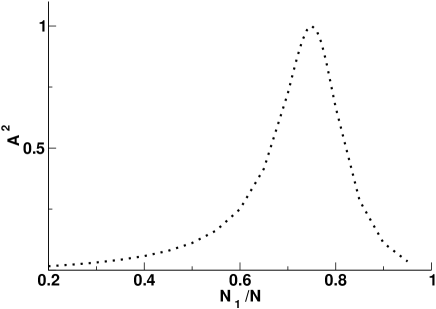
Figure 4: Variance of ${{\mathcal{A}}}={\mathcal{G}}_{a}/{\mathcal{G}}_{s}$ as a function of contact asymmetry reaches maximum at $N_{1}/N=C/2C_{\mu}$ (presented for $N=4$ and $C/C_{\mu}=1.5$). As $N\to\infty$ maximum becomes sharper

In an experiment the number of channels can be adjusted to maximize asymmetry ${\mathcal{A}}$. In a weakly interacting dot with $C/C_{\mu}>2$ the maximum of ${{\mathcal{A}}}^{2}$ is reached at $N_{1}/N=C/2(C-C_{\mu})$, but it is still small ${{\mathcal{A}}}\ll 1$ due to the weak interactions. If the interaction is relatively strong, $C/C_{\mu}<2$ then at $N_{1}/N=C/2C_{\mu}$ the maximum ${{\mathcal{A}}}=1$ is achieved, see Fig. 4. It is this contact width that minimizes the magnitude of $\langle\chi_{2s}\rangle$.

In a realistic quantum dot with symmetric contacts Zumbuhl the interaction is reasonably strong and at intermediate magnetic fields $|\phi\pm\phi^{\prime}|<1$ we have ${{\mathcal{A}}}^{2}={\mathcal{F}}_{-}/{\mathcal{F}}_{+}$. However, it is important to emphasize that if a dot becomes smaller, the ratio $e^{2}/C\Delta$ ($\propto L/a_{B}$ for a dot without gates) can diminish as well. Therefore one could expect that interactions are not necessarily strong and at $1<C/C_{\mu}<2$ it would be important to make the contacts asymmetric to clearly observe a magnetic-field asymmetry. The peak in the Fig. 4 becomes narrower as $N\to\infty$ and the choice of contact width such that $N_{1}/N\approx C/2C_{\mu}$ becomes crucial. This behavior is a consequence of the scaling of the numerator of Eq. (17): the width of this peak as a function of $N_{1}/N$ is proportional to fluctuations $\delta\chi_{2}$ discussed above. Although experiments are often performed with symmetric contacts to avoid parasitic effects of an asymmetric circuit, our results suggest that using contact asymmetry can enhance the magnetic-field asymmetry.

Fluctuations of ${\mathcal{A}}$ can not be found in closed form, since ${\mathcal{F}}_{\pm}$ are complicated functions of $t$ and $\phi$, see Eq. (17). At low temperatures $t\ll 1$ the temperature-dependence of ${\mathcal{F}}_{\pm}$ can be neglected. In the regime $t\gtrsim 1$, more relevant for experiment Zumbuhl (see also discussion in Sec. IV), the fluctuations of ${\mathcal{A}}$ for a dot with symmetric contacts $N_{1}=N_{2}$ can be expressed in terms of linear conductance $g(\phi)$ and its universal fluctuations $\mbox{var }g$:

$$\mbox{var }{\mathcal{A}} = \frac{\phi^{2}\mbox{var }g}{(2+\phi^{2})\mbox{var }g+2(1+\phi^{2})\left(\frac{C}{C_{\mu}}-1\right)^{2}g^{2}},$$ (18)

$$\mbox{var }{\mathcal{A}} = \frac{1}{1+2(g^{2}/\mbox{var }g)(C/C_{\mu}-1)^{2}},\,\,\phi\gg 1.$$ (19)

The high-field limit $\phi\gg 1$ of var ${\mathcal{A}}$ is universal and Eq. (19) is valid for arbitrary temperatures $t$, as long as $T\ll E_{\rm Th}$. However, this value is temperature-dependent due to temperature dependence of UCF. As Eqs. (18,19) demonstrate, measurements of ${\mathcal{A}}$ could serve as a tool to find interaction strength $C_{\mu}/C$. Recently an experiment in micrometer-sized Aharonov-Bohm (AB) rings Bouchiat found ${\mathcal{A}}\approx 0.3$ analyzing the amplitude of the AB-oscillations in the non-linear conductance. This asymmetry was found to be rather insensitive to variation of sample’s conductance $g\gg 1$, which means that the 2nd term in the denominator of Eq. (19) is not large and interactions are rather strong, $C_{\mu}/C\approx 0.9$.

Since the asymmetry parameter ${\mathcal{A}}$ is not sensitive to the fluctuations of the density of states, it probes interactions more directly than ${\mathcal{G}}_{a}$. The symmetrized ${\mathcal{G}}_{s}$ is measured in Zumbuhl on the background of UCF in the linear conductance, so that the interaction strength could be evaluated only from the amplitude of ${\mathcal{G}}_{a}$. Similar to Bouchiat measurement of ${\mathcal{A}}$ in quantum dots would provide a more precise measure of interactions then those of ${\mathcal{G}}_{a},{\mathcal{G}}_{s}$, which we consider below.

For pair correlators of ${\mathcal{G}}_{a}$ and ${\mathcal{G}}_{s}$ all fluctuating quantities of Eq. (11) should be taken into account:

$$\binom{\langle{\mathcal{G}}_{a}(t,\phi){\mathcal{G}}_{a}(t^{\prime},\phi^{\prime})\rangle}{\langle{\mathcal{G}}_{s}(t,\phi){\mathcal{G}}_{s}(t^{\prime},\phi^{\prime})\rangle} = \binom{{\mathcal{F}}_{-}}{{\mathcal{F}}_{+}+\frac{N^{2}}{2N_{1}N_{2}}\left(\frac{C}{C_{\mu}}-\frac{2N_{1}}{N}\right)^{2}}$$ (20)

$$\times \left(\frac{2\pi}{\Delta}\frac{C_{\mu}}{C}\right)^{2}\frac{N_{1}^{3}N_{2}^{3}}{N^{6}}{\mathcal{F}}_{+}.$$

Some properties of these correlators at $t=t^{\prime},\phi=\phi^{\prime}$ were discussed in Ref. PB, . Equation (20) allows one to easily evaluate fluctuations in the non-linear conductance as a function of temperature and flux. For example, at sufficiently high flux difference, correlation functions decay strongly. Similarly to ’magnetic fingerprints’ in the linear conductance meso , the nonlinear conductance is randomized beyond $|\phi-\phi^{\prime}|\sim 1$.

We note some similarities between Eqs. (17) and Eq.(20). Despite these similarities, an important difference is that correlations of ${{\mathcal{A}}}={\mathcal{G}}_{a}/{\mathcal{G}}_{s}$ (see (17)) are not given by a simple ratio of its averaged numerator and denominator of Eq. (20), $\langle{{\mathcal{A}}}^{2}\rangle\neq\langle{\mathcal{G}}_{a}^{2}\rangle/\langle{\mathcal{G}}_{s}^{2}\rangle$. In contrast, to leading order in $1/N\ll 1$ ${\mathcal{G}}_{a}$ and ${\mathcal{G}}_{s}$ are uncorrelated.

Weakly interacting limit. In the limit of weak interactions $C_{\mu}/C\to 0$ and the magnetic field asymmetry in Eq. (20) vanishes. However, even without interactions non-linear conductance exists AK ; KL . The energy scale $eV_{c}\sim\hbar/\tau_{\rm d}$ was argued to be the only energy scale for the crossover from linear to non-linear transport. In the open diffusive samples considered in AK ; KL $eV_{c}\sim E_{\rm Th}$ since $\tau_{\rm d}\sim\tau_{\rm erg}$.

Equation (20) helps us to relate the correlations of non-linear conductances at arbitrary $t,\phi$ and $t^{\prime},\phi^{\prime}$ in weakly interacting dots to those of the linear conductance. In particular, we find that in this limit the ratio of correlation functions of linear and non-linear conductances is constant at fixed $\tau_{\rm d}$. Particularly, for UCF and fluctuations of ${\mathcal{G}}$, we find a universal relation

$$\mbox{var }g=2(\hbar/\tau_{\rm d})^{2}\mbox{ var }{\mathcal{G}}_{s}.$$ (21)

insensitive to temperature $t$ and magnetic flux $\phi$. This relation illustrates the qualitative arguments of AK ; KL that transport coefficients in the non-interacting system scale with $\hbar/\tau_{\rm d}=N\Delta/2\pi$.

In the crossover from weak to strong interactions a typical amplitude of the fluctuations in ${\mathcal{G}}_{s}$ changes from $\delta{\mathcal{G}}_{s}\sim 1/(N\Delta),\delta{\mathcal{G}}_{a}\approx 0$, see Eq. (21), to a value $\delta{\mathcal{G}}_{s},\delta{\mathcal{G}}_{a}\sim 1/(N^{2}\Delta)\cdot\mbox{min }\{1,\sqrt{1/t}\}$. Therefore, in the experiment, the interaction induced scaling of a non-linear response $\delta{\mathcal{G}}_{a}\sim\delta{\mathcal{G}}_{s}$ proportional to $1/N^{2}$ can be observed. In contrast for a non-interacting system we predict (see Eq. (21)) that ${\mathcal{G}}_{a}=0$ and ${\mathcal{G}}_{s}$ is proportional to $1/N$. Indeed, in the experiment by Angers et al.Bouchiat , this observation allows one to evaluate the interaction strength in Aharonov-Bohm rings, $C_{\mu}/C\approx 0.9$.

III.2 Multi-terminal dot

We point out that similarly to two-terminal dots one can consider multi-terminal dots as well. Since ${\mathcal{G}}_{a}$ is very sensitive to interactions and is often easier to find experimentally, we concentrate on a similar anti-symmetric component ${\mathcal{G}}_{a,\alpha\alpha\alpha}$ and on a mixed non-linear conductance ${\mathcal{G}}_{a,\alpha\beta 0}$, a derivative with respect to the gate voltage $V_{0}$ and contact voltage $V_{\beta}$.

One can demonstrate that in two-terminal dots the non-linearity with respect to $V_{0}$ is absent. Indeed, ${\mathcal{G}}_{\alpha\beta 0}$ in Eq. (6) is only due to $u_{0}(\phi)g^{\prime}_{\alpha\beta}(\phi)$. The derivative $u_{0}$ is always field-symmetric, see Eq. (5). In two-terminal dots $g^{\prime}_{\alpha\beta}(\phi)$ is symmetric too, $g^{\prime}_{\alpha\beta}(\phi)=g^{\prime}_{\alpha\beta}(-\phi)$. As a consequence ${\mathcal{G}}_{\alpha\beta 0}$ is even in magnetic field for two-terminal dot (the classical effect of $V_{0}$ in two-terminal samples was considered in Rikken_Wyder ). However, such asymmetry appears in a multi-terminal set-up, since $g^{\prime}_{\alpha\beta}(\phi)\neq g^{\prime}_{\alpha\beta}(-\phi)$.

We find for the variances of ${\mathcal{G}}_{a,\alpha\alpha\alpha}$ and ${\mathcal{G}}_{a,\alpha\beta 0}$,

$$\mbox{var }{\mathcal{G}}_{a,\alpha\alpha\alpha} = \left(\frac{2\pi}{\Delta}\frac{C_{\mu}}{C}\right)^{2}\frac{N_{\alpha}^{3}(N-N_{\alpha})^{3}}{N^{6}}{\mathcal{F}}_{+}{\mathcal{F}}_{-},$$ (22)

$$\mbox{var }{\mathcal{G}}_{a,\alpha\beta 0} = \left(\frac{\pi C_{\mu}}{\nu_{s}e^{2}}\right)^{2}\frac{N_{\alpha}^{2}N_{\beta}^{2}}{N^{4}}{\mathcal{F}}_{-}.$$ (23)

Equation (23) is of particular importance since it can serve to find $C_{\mu}$ in an experiment. This result does not contain an apriori unknown $C$. It is useful to notice that for strongly interacting electrons the effect of gate voltages is weak ($C\to 0$) and therefore voltage difference between gates and the dot can be rather large. Therefore, the non-linear conductance becomes insensitive to the gate voltage and scales with $C_{\mu}\approx C\to 0$. However, for weakly interacting electrons $C_{\mu}\to\nu_{s}e^{2}/\Delta$, the internal potential closely follows the gate voltage and so the effect of gates becomes measurable.

IV Discussion

The results we have obtained can now be compared with results for the linear conductance. From such a comparison we can assert that it is indeed the weakly non-linear transport regime which should be used to extract information on the interaction strength rather than the linear conductance. At finite temperature $t=2\pi T/N\Delta$, in open quantum dots with many ballistic channels, $N\gg 1$, the amplitude of the random linear conductance fluctuations calculated in the strong interaction limit $e^{2}/C\Delta\gg 1$ depends on interactions as $\delta g\sim-t^{2}$, for $t\ll 1$ and $\delta g\sim-1/Nt^{3/2}$ for $t\gg 1$ BLF . On the other hand, random fluctuations of the non-linear conductances ${\mathcal{G}}_{a},{\mathcal{G}}_{s}$ in this limit $e^{2}/C\Delta\gg 1$ are $\propto 1/(N^{2}\Delta)\mbox{ min }\{1,1/t\}$. For a voltage of the order of $eV\propto N\Delta$, the fluctuating contribution of the non-linear component to the current is $\propto{\mathcal{G}}(eV/\Delta)^{2}$ and can be compared with the fluctuating linear contribution $\delta g\,eV/\Delta$. We conclude that for voltages in the interval $\mbox{ min }\{Nt^{2},1/\sqrt{t}\}\ll eV/N\Delta\ll 1$ the transport is still weakly non-linear, but the quantum contribution due to Coulomb interaction to non-linear transport is stronger then the linear contribution. This estimate demonstrates that in dc-transport the effect of Coulomb interactions in open mesoscopic conductors is best investigated in the non-linear regime.

Another important issue is the sensitivity to small magnetic flux, $\phi\ll 1$, when $I(\phi)$ in a two-terminal dot becomes an asymmetric function due to Coulomb interaction. In the experiment $t\gtrsim 0.5$ Zumbuhl , so temperature should be taken into account. Although we do not consider inelastic scattering due to $T\neq 0$, the non-linear conductance ${\mathcal{G}}_{a}(T)$ is temperature dependent since scattering is energy dependent. Of particular interest for the experiment Zumbuhl is the quantity $g_{B-}=(2\nu_{s}e^{3}/h)V{\mathcal{G}}_{a}$ in the limit where ${\mathcal{G}}_{a}(\phi)$ is still linear in flux, $\phi\lesssim 1$, see Fig. 2. We use Eq. (20) and find

$$\mbox{rms }{\mathcal{G}}_{a}(\phi) = \left(\frac{2\pi}{\Delta}\frac{C_{\mu}}{C}\right)\left(\frac{N_{1}^{3}N_{2}^{3}}{N^{10}}\right)^{1/2}\cdot 4\phi$$ (24)

$$\times \left(\int\frac{\pi^{4}t^{4}x^{2}y^{2}(1+y)e^{-x-y}dxdy}{2\sinh^{2}\pi ty\sinh^{2}{\pi tx}}\right)^{1/2}$$

The data obtained at $T=4\mu eV\ll\Delta=7\mu eV$ were fitted to a combination of the zero-temperature results SB ; SZ corresponding to a $\mbox{rms }{\mathcal{G}}_{a}$ given by the first line of (24) with $4\phi$ substituted by $\Phi/\Phi_{0}$ Zumbuhl .

It is noteworthy that a treatment of the crossover leads instead to Eq. (24) with a non-linear conductance $\mbox{rms }{\mathcal{G}}_{a}\propto\phi$, where $\phi\propto\Phi/\Phi_{c}$ is defined by Eq. (2), and not $\Phi/\Phi_{0}$. Indeed, the flux dependence of ${\mathcal{G}}_{a}(\Phi)$ starts to saturate at a scale which is parametrically smaller then $\Phi_{0}$. This is a consequence of the existence of two relevant time-scales, $\tau_{\rm d}$ and $\tau_{\rm erg}$. Thus an attempt to fit the data to a theory of open diffusive samples SZ by substituting $\tau_{\rm erg}\to\tau_{\rm d}$ fails to catch the difference between $\Phi_{0}$ and $\Phi_{c}\propto\Phi_{0}(\tau_{\rm erg}/\tau_{\rm d})^{1/2}$. Being an order-of-magnitude estimate to ballistic quantum dot results, the substitution $\Phi_{c}\to\Phi_{0}$ misses parametric difference between these fields due to the zero-dimensional physics of a chaotic dot. This is especially important if the dependence of the effect on $N$ is considered, and $\mbox{rms }{\mathcal{G}}_{a}\propto N^{-5/2}$ at $T\to 0$.

We also point out that the temperature effect should have appeared even at such low temperatures as $T=4\mu$eV. Indeed, the last factor of Eq. (24) is equal to 1 for $t\ll 1$ and $\sqrt{2}\pi/12t$ at $t\gg 1$. Because of exponential suppression of the integrands at $x,y\sim 1/(\pi t)$, for $t\gtrsim 0.5$ the high temperature asymptotic is a good approximation. Since $\Phi_{c}\propto\sqrt{N}$, the nonlinear conductance as a function of $N$ and $T$ behaves as $\mbox{rms }{\mathcal{G}}_{a}\propto N^{-3/2}T^{-1}$.

To summarize, we discussed the symmetric and anti-symmetric components of non-linear conductance through chaotic two-terminal and multi-terminal quantum dots. Their correlations were found to strongly depend on the interplay between the asymmetry of ballistic contacts and the strength of Coulomb interactions. We discussed the effect of a variation of the gate-voltage on the anti-symmetric component of weakly non-linear conductance through multi-terminal dots. We investigated the conditions on sample contacts, magnetic field and temperature under which the (relative) magnetic field asymmetry is maximal and thus most easy to detect.

We thank David Sánchez for his valuable comments. We acknowledge discussions with Piet Brouwer, Dominik Zumbühl, and Hélène Bouchiat. This work was supported by the Swiss National Science Foundation, the Swiss Center for Excellence MaNEP and the STREP project SUBTLE.

References

- (1) L. Onsager, Phys. Rev. 38, 2265 (1931), H. B. G. Casimir, Rev, Mod. Phys. 17, 343 (1945).
- (2) M. Büttiker, Phys. Rev. Lett. 57, 1761 (1986).
- (3) Mesoscopic phenomena in solids, ed. B. L. Altshuler, P. A. Lee, and R. A. Webb, North-Holland (1991)
- (4) B. L. Altshuler and A. G. Aronov in Electron-electron interactions in disordered systems, ed. A. L. Efros and M. Pollak, North-Holland (1985), 1.
- (5) P. W. Brouwer, A Lamacraft, and K. Flensberg, Phys. Rev. B 72, 075316 (2005).
- (6) B. L. Altshuler and D. Khmelnitskii, Pis’ma Zh. Eksp. Teor. Fiz. 42, 291 (1985) [Sov. Phys. JETP Lett. 42, 359 (1985)].
- (7) D. E. Khmelnitskii and A. I. Larkin, Physica Scripta, T14, 4 (1986); Zh. Eksp. Teor. Phys. 91, 1815 (1986) [Sov. Phys. JETP 64, 1075 (1986)].
- (8) V. I. Fal’ko and D. E. Khmelnitskii, Zh. Eksp. Teor. Fiz. 95, 328 (1989) [Sov. Phys. JETP, 68, 186 (1989)].
- (9) D. Sánchez and M. Büttiker, Phys. Rev. Lett. 93, 106802 (2004).
- (10) B. Spivak and A. Zyuzin, Phys. Rev. Lett. 93, 226801 (2004).
- (11) M. L. Polianski and M. Büttiker, Phys. Rev. Lett. 96, 156804 (2006).
- (12) J. Wei, M. Shimogawa, Z. Wang, I. Radu, R. Dormaier, and D. H. Cobden, Phys. Rev. Lett. 95, 256601 (2005).
- (13) C. A. Marlow, R. P. Taylor, M. Fairbanks, I. Shorubalko, and H. Linke, Phys. Rev. Lett. 96, 116801 (2006).
- (14) D. Zumbühl, C. M. Marcus, M. P. Hanson, A. C. Gossard, Phys. Rev. Lett. 96, 206802 (2006).
- (15) R. Leturcq, D. Sánchez, G. Gotz, T. Ihn, K. Ensslin, D. C. Driscoll, A. C. Gossard, Phys. Rev. Lett. 96, 126801 (2006).
- (16) L. Angers, E. Zakka-Bajjani, R. Deblock, S. Gueron, A. Cavanna, U. Gennser, H. Bouchiat, and M. L. Polianski, to be published in Phys. Rev. B
- (17) M. Büttiker and D. Sánchez, Intl. J. Quant. Chem. 105, 906 (2005).
- (18) A. De Martino, R. Egger, and A. M. Tsvelik, Phys. Rev. Lett. 97, 076402 (2006)
- (19) A. V. Andreev and L. I. Glazman, Phys. Rev, Lett. 97, 266806 (2006).
- (20) C. W. J. Beenakker, Rev. Mod. Phys. 69, 731 (1997).
- (21) I. L. Aleiner, P. W. Brouwer, and L. I. Glazman, Phys. Rep. 358, 309 (2002).
- (22) P. W. Brouwer, C. W. J. Beenakker, J. Math. Phys. 37, 4904 (1996).
- (23) M. L. Polianski and P. W. Brouwer, J. Phys. A: Math. Gen. 36, 3215 (2003).
- (24) T. Ludwig, Ya. M. Blanter, A. D. Mirlin, Phys. Rev. B 70, 235315 (2004).
- (25) S. Adam, M. L. Polianski, X. Waintal, and P. W. Brouwer, Phys. Rev. B 66, 195412 (2002).
- (26) K. Frahm and J-L. Pichard, J. Phys. (France) I 5, 847 (1995).
- (27) M. Büttiker, J. Phys. Cond. Mat. 5, 9361 (1993)
- (28) T. Christen and M. Büttiker, Europhys. Lett. 35, 523 (1996).
- (29) T. Christen, Phys. Rev. B 55, 7606 (1997).
- (30) M. Büttiker, A. Prêtre, and H. Thomas, Phys. Rev. Lett. 70, 4114 (1993).
- (31) M. Büttiker and M. L. Polianski, J. Phys. A: Math. Gen. 38, 10559 (2005).
- (32) M. G. Vavilov and I. L. Aleiner, Phys. Rev. B 64, 085115 (2001).
- (33) D. Sánchez, M. Büttiker, Phys. Rev. B 72, 201308(R) (2005).
- (34) P. W. Brouwer, S. A. van Langen, K. M. Frahm, M. Büttiker, and C. W. J. Beenakker, Phys. Rev. Lett. 79, 913 (1997).
- (35) P. W. Brouwer, Phys. Rev. B 58, 10135 (1998).
- (36) M. Moskalets and M. Buẗtiker Phys. Rev. B 72, 035324 (2005)
- (37) P. W. Brouwer and S. Rahav, Phys. Rev. B 74, 085313 (2006).
- (38) P. W. Brouwer and M. Büttiker, Europhys. Lett. 37, 441 (1997).
- (39) G. L. J. Rikken and P. Wyder, Phys. Rev. Lett. 94, 016601 (2005).