Analytical Study of Electronic Structure in Armchair Graphene Nanoribbons

Abstract

We present the analytical solution of the wavefunction and energy dispersion of armchair graphene nanoribbons (GNRs) based on the tight-binding approximation. By imposing hard-wall boundary condition, we find that the wavevector in the confined direction is discretized. This discrete wavevector serves as the index of different subbands. Our analytical solutions of wavefunction and associated energy dispersion reproduce the numerical tight-binding results and the solutions based on the $\bf k\cdot p$ approximation. In addition, we also find that all armchair GNRs with edge deformation have energy gaps, which agrees with recently reported first-principles calculations.

I Introduction

Graphene, as a promising candidate of future nanoelectronic components, has recently attracted intensive research attention.1 ; 2 ; 3 ; 4 ; 5 ; 6 Graphene consists of a single atomic layer of graphite, which can also be viewed as a sheet of unrolled carbon nanotube. Several anomalous phenomena ranging from half-integer quantum Hall effect, non-zero Berry’s phase 2 , to minimum conductivity 3 , have been observed in experiments. These unusual transport properties may lead to novel applications in carbon-based nanoelectronics. In addition, the carriers in graphene behave as massless relativistic particles with an effective ‘speed of light’ $c_{*}\approx 10^{6}m/s$ within the low-energy range ($\varepsilon<0.5eV$). 2 These massless Dirac fermions in graphene manifest various quantum electrodynamics (QED) phenomena in the low energy range such as Klein paradox phenomenon. 6 Ribbons with a finite width of graphene, referred to as graphene nanoribbons (GNRs), have also been studied extensively. JPSJ96 ; KNPRB96 ; KWPRB99 ; MEPRB06 ; LouiePRL06 ; LouieNat06 ; YMPRB99 ; LBPRB06 Recent experiments by using the mechanical method 2 ; 3 and the epitaxial growth method 4 ; CBJPCB04 show it is possible to make GNRs with various widths.

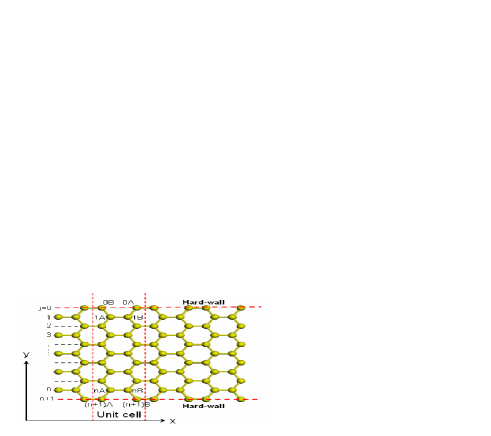
Figure 1: (color online) Structure of an armchair graphene nanoribbon, consisting of sublattices, A and B. The width of the armchair GNR is $n$. Every unit cell contains $n$ number of A and B sublattices. Two additional hard walls ($j=0,n+1$) are imposed on both edges.

The carbon atoms on the edge of GNRs have two typical topological shapes, namely armchair and zigzag. The analytical wavefunction and energy dispersion of zigzag nanoribbons have been derived by several research groups. KSJPSJ06 ; APL06 For armchair GNRs, the analytical forms of wavefunctions within the low energy range have been worked out based on the effective-mass approximation. LBPRB06 It is predicted that all zigzag GNRs are metallic with localized states on the edges, KNPRB96 ; KWPRB99 ; KSJPSJ06 ; APL06 while armchair GNRs are either metallic or insulating, depending on their widths. JPSJ96 ; KNPRB96 ; KWPRB99 ; MEPRB06 ; KSJPSJ06 ; LBPRB06 To-date, there is no general expression of the wavefunction in armchair GNRs. In this paper, we derive a general analytical expression of wavefunction and eigen-energy in armchair GNRs applicable to various energy ranges. In part II, we focus on perfect armchair GNRs without any edge deformation and derive the energy dispersion by imposing the hard-wall boundary condition. Due to the quantum confinement, the spectrum breaks into a set of subbands and the wavevector along the confined direction becomes discretized. We observe that the electronic structure of perfect armchair GNRs strongly depends on the width of the ribbon. The system, for instance, is metallic when $n=3m+2$ and is insulating otherwise, where $m$ is an integer. JPSJ96 ; KNPRB96 ; KWPRB99 ; MEPRB06 ; KSJPSJ06 ; LBPRB06 Furthermore, we study the low energy electronic structure. The linear dispersion relation is observed in armchair GNRs. In part III, we evaluate the effect of deformations on the edges on the electronic structure of armchair GNRs. Calculation results based on the derived analytical wavefunction show that all armchair GNRs have nonzero energy gaps due to the variation of hopping integral near the edges. This observation is in line with the recently reported first-principle calculations. LouiePRL06

II Perfect armchair graphene nanoribbon

The structure of armchair GNRs consists two types of sublattices A and B as illustrated in Fig. 1. The unit cell contains $n$ A-type atoms and $n$ B-type atoms. Based on the translational invariance, we choose plane wave basis along the $x$ direction. Within the tight-binding model, the wavefunctions of A and B sublattices can be written as

$$\left|\psi\right\rangle_{A}=\frac{1}{{N_{A}}}\sum\limits_{x_{A_{i}}}{\sum\limits_{i=1}^{n}{e^{ik_{x}x_{A_{i}}}}}\phi_{A}(i)\left|{A_{i}}\right\rangle$$

$$\left|\psi\right\rangle_{B}=\frac{1}{{N_{B}}}\sum\limits_{x_{B_{i}}}{\sum\limits_{i=1}^{n}{e^{ik_{x}x_{B_{i}}}}}\phi_{B}(i)\left|{B_{i}}\right\rangle,$$ (1)

where $\phi_{A}(i)$ and $\phi_{B}(i)$ are the components for A and B sublattices in the $y$ direction, which is perpendicular to the edge. $\left|{A_{i}}\right\rangle$ and $\left|{B_{i}}\right\rangle$ are the wave functions of the $p_{z}$ orbit of a carbon atom located at A and B sublattices, respectively. To solve $\phi_{A}(i)$ and $\phi_{B}(i)$, we employ the hard-wall boundary condition

$$\phi_{A}(0) = \phi_{B}(0)=0$$

$$\phi_{A}(n+1) = \phi_{B}(n+1)=0.$$ (2)

Choosing $\phi_{A}(i)=\phi_{B}(i)=\sin(\frac{{\sqrt{3}q_{y}a}}{2}i)$ and substituting them into Eq. (2), we get

$$q_{y}=\frac{2}{{\sqrt{3}a}}\frac{{p\pi}}{{n+1}},\ \ \ p=1,2,\cdots,n.$$ (3)

$q_{y}$ is the discretized wavevector in the $y$ direction and $a=1.42\AA$ is the bond length between carbon atoms. To obtain the normalized coefficients, $N_{A}$ and $N_{B}$, we introduce the normalization condition

$${}_{A}\left\langle\psi\right|\left.\psi\right\rangle_{A}=_{B}\left\langle\psi\right|\left.\psi\right\rangle_{B}=1.$$

It is straightforward to obtain $N_{A}=N_{B}=\sqrt{\frac{N_{x}(n+1)}{2}}$, where $N_{x}$ is the number of unit cells along the $x$ direction. The total wavefunction of the system can be constructed by the linear combination of $\psi_{A}$ and $\psi_{B}$

$$\left|\psi\right\rangle=C_{A}(\sqrt{\frac{2}{{N_{x}(n+1)}}}\sum\limits_{x_{A_{i}}}{\sum\limits_{i=1}^{n}{e^{ik_{x}x_{A_{i}}}}}\sin(\frac{{\sqrt{3}q_{y}a}}{2}i)\left|{A_{i}}\right\rangle)$$

$$+C_{B}(\sqrt{\frac{2}{{N_{x}(n+1)}}}\sum\limits_{x_{B_{i}}}{\sum\limits_{i=1}^{n}{e^{ik_{x}x_{B_{i}}}}}\sin(\frac{{\sqrt{3}q_{y}a}}{2}i)\left|{B_{i}}\right\rangle).$$

(4)

Under the tight binding approximation, the Hamiltonian of the system is

$$H=\sum\limits_{i}{\varepsilon_{i}}\left|i\right\rangle\left\langle i\right|-t_{i,j}\sum\limits_{<i,j>}{(\left|{i}\right\rangle\left\langle{j}\right|)},$$ (5)

where $\left\langle{i},{j}\right\rangle$ denotes the nearest neighbors.

In perfect armchair GNRs, we set $t_{i,j}=t$ and ${\varepsilon_{i}}=\varepsilon$. By Substituting Eq. (4) and Eq. (5) into the Schrodinger equation, we can easily obtain the following matrix expression:

$$\left({\begin{array}[]{*{20}c}\varepsilon&\mu\\ {\mu^{*}}&\varepsilon\\ \end{array}}\right)\left({\begin{array}[]{*{20}c}{C_{A}}\\ {C_{B}}\\ \end{array}}\right)=E\left({\begin{array}[]{*{20}c}{C_{A}}\\ {C_{B}}\\ \end{array}}\right),$$ (12)

where $\mu=_{A}\left\langle\psi\right|H\left|\psi\right\rangle_{B}=t(2e^{ik_{x}\frac{{a}}{2}}\cos(\frac{{\sqrt{3}a}}{2}q_{y})+e^{-ik_{x}a})$. Solving Eq. (6), we get the energy dispersion and wavefunction as

$$E=\varepsilon\pm\left|\mu\right|,$$

$$\left|\psi\right\rangle_{\pm}=\frac{{\sqrt{2}}}{2}(\left|\psi\right\rangle_{A}\pm\sqrt{\frac{{\mu^{*}}}{\mu}}\left|\psi\right\rangle_{B}).$$ (13)

Here, $\pm$ denotes the conduction and valance bands, respectively. $-\frac{\pi}{2}\leq\frac{{3k_{x}a}}{2}\leq\frac{\pi}{2}$ is required within the first Brillion zone. These results are valid for various energy ranges.

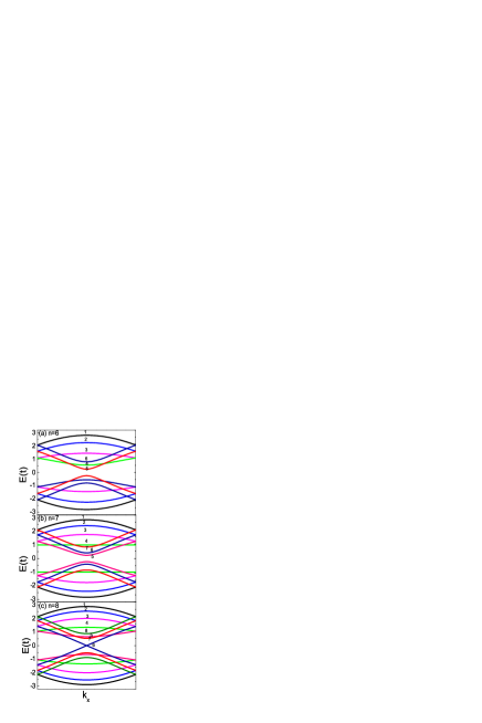
Figure 2: (color online) Electronic structures of perfect armchair GNRs with various widths, (a) n=6 (b) 7 and (c) 8, respectively. The wavevector is normalized based on the primitive translation vector of individual GNRs. The value of $p$ for each subband is labeled in the figure.

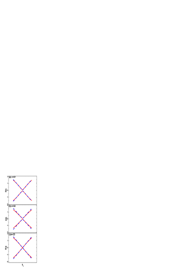
Figure 3: (color online) The first conductance and valence bands within the first Brillion zone: exact solutions from Eq. (7) (red solid line) and low-energy approximation from Eq. (10) (blue dash line) for armchair GNRs with various widths, (a) $n=21$ (b) $n=22$ (c) $n=23$, respectively. The wavevector is normalized based on the primitive translation vector of individual GNRs.

Fig. 2 shows the energy dispersion for perfect armchair GNRs with width $n=6,7$ and $8$. Here, we set $\varepsilon=0$. The results are the same as those obtained by using the numerical tight-binding method. The electronic structures of armchair GNRs depend strongly on their widths. When $n=8$, the lowest conduction band and the upmost valence band touch at the Dirac point, which leads to the metallic behavior of $n=8$ armchair GNRs. Armchair GNRs, however, are insulating when $n=6$ and $n=7$. Armchair GNRs with the width of $n=3m+2$ ($m$ is an integer) are generally metallic and otherwise are insulating. KNPRB96 ; LBPRB06 In addition, we observe several interesting features in the band structures of armchair GNRs.

(i) If $n$=7, a flat conduction/valence band ($p=4$) exists as shown in Fig. 2 (b). Such a flat band generally corresponds to $\frac{{p}}{{n+1}}=\frac{1}{2}$ or equivalently $\cos\frac{{p\pi}}{{n+1}}=0$. The energy dispersion becomes independent of $k_{x}$ and the eigen-energy always equals $\pm\left|t\right|$. Flat band, in general, exists only when $n$ is odd.

(ii) The subbands can be labeled by the quantum number $p$. Combined with the wave number $k_{x}$ along the $x$ direction, the quantum number $p$ can be used to define the chirality of the electrons in quasi-1D graphene ribbons similar to that in 2D graphene. To identify different subbands, we need the the quantum number $p_{i}$ of the $i$th conduction/valence band. Here, the definition of the sequence of subbands is referred to as the value of eigen-energy, $E_{C}$, in the center of first Brillion zone ($k_{x}=0$),

$$E_{C}=\pm t\left|{2\cos\frac{{p\pi}}{{n+1}}+1}\right|.$$ (14)

For the metallic armchair GNRs with width $n=3m+2$ when $\frac{{p\pi}}{{n+1}}=\frac{2\pi}{3}$ or equivalently $p=2m+2$, the energy gap between conduction and valence bands is zero. Therefore, $p_{1}=2m+2$ corresponds to the first conduction/valence band in $n=3m+2$ GNRs. For the second conduction/valence bands, $E_{C}$ should have the minimal nonzero value compared to the third or even higher band. After analyzing the value of $E_{C}$, we find that $p_{2}=2m+3$, $p_{3}=2m+1$ for metallic armchair GNRs ($n=3m+2$). By similar analysis, for $n>10$, we can obtain $p_{1}=2m+1$, $p_{2}=2m$, $p_{3}=2m+2$ for $n=3m$ armchair GNRs and $p_{1}=2m+1$, $p_{2}=2m+2$, $p_{3}=2m$ for $n=3m+1$ armchair GNRs, respectively. For all subbands, there is no general rule of the subband index $p$.

(iii) Lots of research interest have been focusing on the energy dispersion and wavefunction of 2D graphene and 1D GNRs within the low-energy range. 2 ; LouiePRL06 ; LBPRB06 Low-energy electrons behaves as massless relativistic particles in a 2D infinite graphene system. 1 ; 2 ; 3 ; 6 ; LBPRB06 Whether electrons keep their relativistic property when they are confined in quasi-1D graphene nanoribbons is an interesting issue. In what follows, we will focus on the expansion of our analytical expressions to the low energy limit. When $\frac{{p\pi}}{{n+1}}\to\frac{2}{3}\pi$ and $\frac{{3k_{x}a}}{2}\to 0$, we rewrite the eigenenergy in Eq. (7) as

$$E\approx\pm{\textstyle{3\over 2}}at\sqrt{k_{x}^{2}+\tilde{q}_{y}^{2}}\approx\pm\hbar v_{F}k,$$ (15)

where $\tilde{q}_{y}(p)=\frac{2}{{\sqrt{3}a}}(\frac{{p\pi}}{{n+1}}-\frac{2}{3}\pi)$, $p$ is the subband index. This low energy expansion generates the $E\propto k$ linear dispersion, with Fermi velocity $v_{F}\approx 10^{6}m/s$. This expression reproduces the result of $\bf k\cdot p$ approximation. LBPRB06 Note that the wavevector in the confined direction ($\tilde{q}_{y}$) is discretized, corresponding to different subbands. What is worthy mentioning is that this energy dispersion works well only at the low-energy limit. By substituting the value of $p_{1}$ into Eq. (9), we get the low energy expansion of the first conduction/valence band for armchair GNRs as

$$E_{1}(3m)\mathop{\approx}\limits^{k_{x}\to 0} \pm {\textstyle{3\over 2}}at\sqrt{k_{x}^{2}+(\frac{{2\pi}}{{3\sqrt{3}(3m+1)a}})^{2}}$$

$$E_{1}(3m+1)\mathop{\approx}\limits^{k_{x}\to 0} \pm {\textstyle{3\over 2}}at\sqrt{k_{x}^{2}+(\frac{{2\pi}}{{3\sqrt{3}(3m+2)a}})^{2}}$$

$$E_{1}(3m+2)\mathop{\approx}\limits^{k_{x}\to 0} \pm \frac{{3at}}{2}k_{x}.$$ (16)

Figure 4: Local density of the states in the first conduction/valence band at $k_{x}=0$ for armchair GNRs with various widths, (a) $n$=50 (b) $n=51$ and (c) $n=52$, respectively. (These values of $n$ are so chosen to match the results in reference LBPRB06 )

Fig. 3 shows the quality of low energy approximation. For large width armchair GNRs, low energy approximation seems work well except the edge of first Brillion Zone. As the width gets larger, the quantum confinement due to the edge becomes less important and the 1D nanoribbons tend to behave like 2D graphene. For large $n$, as expected, the band structure generates the linear dispersion relationship, $E\propto k_{x}$, in the low-energy limit.

In addition, from the expression of wavefunction, we also obtain the local density of electronic states in perfect armchair GNRs, $P_{A}(i)=P_{B}(i)\propto\sin^{2}(\frac{{p\pi}}{{n+1}}i)$ . Fig. 4 shows the squared wave functions of the lowest conduction band at the center of first Brillion Zone. Note that Fig. 4(a) and (c) reproduce the results of the $\bf k\cdot p$ approximation. LBPRB06 The state density oscillates as a function of the lattice position. The oscillation period is related to $\frac{{n+1}}{p}$. For $n=3m+2$ armchair GNRs, the oscillation period is just 3, which is shown clearly in Fig. 4(a). For $n=3m$, $3m+1$ armchair GNRs, we should write $\frac{{n+1}}{p}$ into an irreducible form $\frac{\alpha}{\beta}$. The oscillation period then equals $\alpha$, which is the numerator of the irreducible form of $\frac{{n+1}}{p}$. To match the results presented in LBPRB06 , we choose $n=51$ and $n=52$ as an example. We get $i=51$ and $i=52$, respectively. As shown in Fig. 4(b) and (c), the oscillation period of state density for $n=51$ and $n=52$ armchair GNRs equals their width.

III Energy Gap and Wavefunction for Edge-deformed GNRs

Because every atom on the edge has one dangling bond unsaturated, the characteristics of the $C-C$ bonds at the edges can change GNRs’ electronic structure dramatically. MEPRB06 ; TKPRB00 To determine the band gaps of GNRs on the scale of nanometer, edge effects should be considered carefully. The change of edge bonds length and angle can lead to considerable variations of electronic structure, especially within the low energy range. LouiePRL06 ; LouieNat06 In previously reported work, the edge carbon atoms of GNRs are all passivated by hydrogen atoms or other kinds of atoms/molecules. LBPRB06 ; MEPRB06 ; TKPRB00 ; LouiePRL06 ; LouieNat06 The bonds between hydrogen and carbon are different from those $C-C$ bonds. Accordingly, the transfer integer of the $C-H$ bonds and on-site energy of carbon atoms at the edges are expected to differ from those in the middle of GNRs. The bond lengths between carbon atoms at the edges are predicted to vary about $3\%-4\%$ when hydrogenerated. LouiePRL06 Correspondingly, the hopping integral increases about $12\%$ extracted from the analytical tight binding expression. DPPRB95 ; LouiePRL06 To evaluate the effect of various kinds of edge deformation, we carried out general theoretical calculation and analysis with our analytical solution of armchair GNRs. In general, we can set the variation of the transfer integer and on-site energy as $\delta t_{i,j}$, $\varepsilon_{i}$ for the $i$th A-type or B-type carbon atom in the unit cell. The Hamiltonian of the GNRs with deformation on the edge can be rewritten as

$$H=\varepsilon_{i}\sum\limits_{i}{\left|i\right\rangle}\left\langle i\right|-\sum\limits_{<i,j>}{(t+\delta t_{i,j})}\left|i\right\rangle\left\langle j\right|$$ (17)

It is readily to obtain the energy dispersion and wavefunction by solving the Schrodinger equation

$$E=\gamma\pm\left|{\mu+\delta\mu}\right|$$

$$\left|\psi\right\rangle_{\pm}=\frac{{\sqrt{2}}}{2}(\left|\psi\right\rangle_{A}\pm\sqrt{\frac{{(\mu+\delta\mu)^{*}}}{{\mu+\delta\mu}}}\left|\psi\right\rangle_{B}),$$ (18)

where $\gamma=\frac{2}{{n+1}}\sum\limits_{i=1}^{n}{\varepsilon_{i}}\sin^{2}(\frac{{p\pi}}{{n+1}}i)$ is the energy shift originating from the variation of on-site energy, while the energy shift from the hopping integral variation is

$$\delta\mu=-\frac{{2t}}{{n+1}}\sum\limits_{i=1}^{n}[\delta t_{i(A)i(B)}\sin^{2}(\frac{{p\pi}}{{n+1}}i)e^{-ik_{x}a}$$

$$+\delta t_{i(A)i-1(B)}\sin(\frac{{p\pi}}{{n+1}}i)\sin(\frac{{p\pi}}{{n+1}}(i-1))e^{\frac{{ik_{x}a}}{2}}$$

$$+\delta t_{i(A)i+1(B)}\sin(\frac{{p\pi}}{{n+1}}i)\sin(\frac{{p\pi}}{{n+1}}(i+1))e^{\frac{{ik_{x}a}}{2}}].$$

Such a general expression could include various kinds of edge deformations, ranging from the quantum confinement effect due to the finite width, to the effect of saturated atoms or molecules attached to edge carbon atoms. This result shows that the deformation leads to a considerable deviation of the energy dispersion relation and wavefunction of the deformed system from those in perfect armchair GNRs. The local state density on both kinds of sublattices, however, remains the same as that in perfect armchair GNRs. The reason is that the wavefunctions of sublattices A and B change their relative phases, but keep the magnitudes unchanged. The variations from both the on-site energy and hopping integral contribute to the energy shift, while, the change of on-site energy has no contribution to the wavefunction as shown in Eq. (8). To verify our findings, we reproduce the energy gap observed in the recent work LouiePRL06 by considering only the variation of hopping integrals of the bonds on the edges ($\delta t_{11}=\delta t_{nn}=\delta t$, others equals zero). The corresponding energy gaps for different width ribbons are as follows:

$$\Delta_{3m} = \Delta_{3m}^{0}-\frac{{8\delta t}}{{3m+1}}\sin^{2}\frac{{m\pi}}{{3m+1}},$$

$$\Delta_{3m+1} = \Delta_{3m+1}^{0}+\frac{{8\delta t}}{{3m+2}}\sin^{2}\frac{{(m+1)\pi}}{{3m+2}},$$

$$\Delta_{3m+2} = \Delta_{3m+2}^{0}+\frac{{2\delta t}}{{m+1}},$$ (20)

where $\Delta_{3m}$, $\Delta_{3m+1}$ and $\Delta_{3m+2}$ are the energy gaps of perfect armchair GNRs. Their values can be extracted from Eq.(8): $2t\left|{2\cos\frac{{(2m+1)\pi}}{{3m+1}}+1}\right|$, $2t\left|{2\cos\frac{{(2m+1)\pi}}{{3m+2}}+1}\right|$ and $0$. This result suggests all armchair graphene ribbons with edge deformation have nonzero energy gaps and are insulating correspondingly.

IV Conclusion

In this paper, we study the electronic states of armchair GNRs analytically. By imposing the hard-wall boundary condition, we find the analytical solution of wavefunction and energy dispersion in armchair GNRs based on the tight-binding approximation. Our results reproduce the numerical tight-binding calculation results and the solutions using the effective-mass approximation. We also derive the low-energy approximation of the energy dispersion, which matches the exact solution except for the edge of first Brillion zone. The linear energy dispersion is observed in armchair GNRs in the low energy limit. In addition, we also evaluate the impact of the edge deformation on GNRs and derive a general expression of wavefunction and energy dispersion. We can reproduce the energy gap for hydrogenerated armchair GNRs presented in LouiePRL06 . When we consider the edge deformation, all armchair GNRs have nonzero energy gaps and thus are insulting. Overall, the derived analytical form of the wavefunction can be used to quantitatively investigate and predict various properties in armchair graphene ribbons.

References

- (1) K. S. Novoselov, A. K. Geim, S. V. Morozov, D. Jiang, Y. Zhang, S. V. Dubonos, I. V. Grigorieva, and A. A. Firsov, Science 306, 666 (2004).
- (2) K. S. Novoselov, A. K. Geim, S. V. Morozov, D. Jiang, M. I. Katsnelson, I. V. Grigorieva, S. V. Dubonos and A. A. Firsov, Nature 438, 197 (2005).
- (3) Yuanbo Zhang, Yan-Wen Tan, Horst L. Stormer1, and Philip Kim, Nature 438, 201 (2005).
- (4) Claire Berger, Zhimin Song, Xuebin Li, Xiaosong Wu, Nate Brown, Cécile Naud, Didier Mayou, Tianbo Li, Joanna Hass, Alexei N. Marchenkov, Edward H. Conrad, Phillip N. First and Walt A. de Heer, Science 312, 1191 (2006).
- (5) Taisuke Ohta, Aaron Bostwick, Thomas Seyller, Karsten Horn and Eli Rotenberg, Science 313, 951 (2006).
- (6) M. I. Katsnelson, K. S. Novoselov, A. K. Geim, Nature 2, 620 (2006).
- (7) M. Fujita, K. Wakabayashi, K. Nakada, K. Kusakabe, J. Phys. Soc. Jpn 65, 1920 (1996).
- (8) K. Nakada, M. Fujita, G. Dresselhaus, M. S. Dresselhaus, Phys. Rev. B 54, 17954 (1996).
- (9) K. Wakabayashi, M. Fujita, H. Ajiki, M. Sigrist, Phys. Rev. B 59, 8271 (1999).
- (10) M. Ezawa, Phys. Rev. B (73), 045432 (2006).
- (11) Y.-W. Son, M. L. Cohen and S. G. Lioue, Phys. Rev. Lett. (97), 216803 (2006).
- (12) Y.-W. Son, M. L. Cohen and S. G. Lioue, Nature (London)(444), 347 (2006).
- (13) Y. Miyamoto, K. Nakada, M. Fujita, Phys. Rev. B 59, 9858 (1999).
- (14) L. Brey and H. A. Fertig, Phys. Rev. B (73), 235411 (2006).
- (15) C. Berger et al., J. Phys. Chem. B (108), 19912 (2004).
- (16) Ken-ichi SASAKI, Shuichi MURAKAMI and Riichiro SAITO, J. Phys. Soc. Jpn. 75 (2006) 074713.
- (17) K. Sasaki, S. Murakami and R. Saito, Appl. Phys. Lett. (88), 113110 (2006).
- (18) D. Porezag et al., Phys. Rev. B (51), 12947 (1995).
- (19) T. Kawai, Y. Miyamoto, O. Sugino, and Y. Koga, Phys. Rev. B (62), R16349 (2000).